Combining Active Learning and Mathematical Programming: a hybrid approach for Transprecision Computing

(1)

ALMA MATER STUDIORUM

UNIVERSITÀ DI BOLOGNA

SCUOLA DI INGEGNERIA E ARCHITETTURA

Corso di Laurea Magistrale in Ingegneria Informatica

Combining Active Learning and Mathematical Programming: a

hybrid approach for Transprecision Computing

TESI DI LAUREA

in

INTELLIGENT SYSTEMS M

Relatore

Prof.ssa Milano Michela

Presentata da

Bambini Alberto

Correlatore

Dott. Borghesi Andrea

Anno Accademico 2018/19

Sessione III

(2)

(3)

Summary

Summary ... I List of tables ... III List of figures ... V 1 Introduction ... 1 2 Transprecision Computing ... 3 2.1 Concept ... 3 2.2 OPRECOMP ... 5 2.3 FlexFloat ... 6 3 Active Learning ... 9 3.1 Concept ... 9 4 Mathematical Programming ... 13

4.1 CPLEX and DOcplex ... 14

4.2 Empirical Model Learning ... 14

5 Project and objectives ... 17

5.1 Optimization Model ... 18

5.2 Machine Learning Model and Active Learning ... 19

5.3 Benchmarks and Variables Graph ... 21

5.4 Structure... 25

6 Results ... 39

6.1 Consistency Tests ... 40

6.2 Neighborhood search Tests ... 46

6.3 Active Learning Trend Tests ... 48

(4)

II

Appendices ... 61

I. Convolution executions ... 61

II. Correlation executions ... 66

(5)

List of tables

Table 1: Experiment report structure ... 39

Table 2: Correlation execution data, target 10-7 (1) ... 41

Table 7: Correlation execution data, target 10-5, all neighborhood search versions ... 47

Table 8: Convolution execution data, target 10-15 ... 49

Table 9: Convolution execution data, target 10-20_{... 51}

Table 10: Correlation execution data, target 10-5_{... 52}

Table 11: Correlation execution data, target 10-10_{... 53}

(6)

List of tables

(7)

List of figures

Figure 1: Discrete precision approximation in a time interval ... 5

Figure 2: The complete coverage of the framework (Malossi, et al., 2018) ... 6

Figure 3: FlexFloat internal representation of a floating-point type ... 7

Figure 4: Pool-based active learning cycle ... 10

Figure 5: Visualization of the length limits of the mantissa on a 64-bits long backend ... 17

Figure 6: Regressor network for a 4 variables configuration ... 20

Figure 7: Variables Graph visualization of the correlation benchmark ... 23

Figure 8: General control flow of the script ... 26

Figure 9: Training set creation flow diagram ... 27

Figure 10: Optimization model solving algorithm, phase one ... 29

Figure 11: Optimization model solving algorithm, phase two (two versions) ... 30

Figure 12: Distribution for sampling the deviation of a single value in a configuration ... 34

Figure 13: Error and predicted error trends for each execution. Green dots correspond to the best solutions, yellow dots are generated solutions. ... 44

Figure 14: Bits sum trends for each execution. The red line identifies the sum of the optimal solution, while the green dots identify the sums for each best solution ... 45

Figure 15: Regressor metrics (left), Classifier metrics (right) (1) ... 50

(8)

List of figures

(9)

Introduction

1 Introduction

The energy consumption of computing systems is constantly growing and is a prevalent issue in a world tht increasingly values energy efficiency and sustainability. In this context, approximate computing techniques have been proposed in a variety of domains to design, both hardware and software, systems capable of making a compromise between the quality of the computed results and energy efficiency by which these results are produced. Among these strategies particular attention has been paid to precision scaling, a methodology which consists of changing the bit-width of program data to reduce storage and/or computing requirements (Tagliavini, Marongiu, & Benini, 2018).

The objective of this paper is to be a chapter in the development process of such techniques by joining an European project known as OPRECOMP and, more precisely, by becoming an integral part of the experimentations carried out by the Department of Computer Science and Engineering (DISI) of the University of Bologna in the purview of the application of AI and optimization techniques to regulate the energetic efficiency of high precision computations. In particular, this paper explores the possibility of applying a hybrid approach between Active Learning and Mathematical Programming to Transprecision Computing. This would entail embedding a machine learning model trained by means of an Active Learning approach into an optimization model to automatically and intelligently tweak the representation of floating-point numerical data. This project aims to lower the energetic expenditure of every single intermediate computation in a given program, while also avoiding errors that are systematically introduced when manipulating variables using this technique, and ensure that they do not exceed a maximum acceptable error rate decided prior.

This report is structured in three parts, spanning from the base concepts to the actual experiments and results. The first part (chapters 2, 3, and 4) covers the concepts of Transprecision Computing, Active Learning, and Mathematical Programming, while also presenting OPRECOMP, its goals and how they are related to this thesis. The libraries and tools used to develop and test this project are also presented here, with particular

(10)

Introduction

2

attention on how FlexFloat (the Transprecision library) and EMLlib (a library to embed Ml models into optimization models) work internally, to explain and justify some decisions that were made during development.

The second part (chapter 5) analyzes and explores in detail the structure of the execution flow of the Python script produced for the experiments that will be mentioned in the final part. It first introduces the optimization problem and the model that was built to solve it and gives a full overview of the Machine Learning models, their structure and the reason why Active Learning proved to be essential to achieve good results. The paper then introduces the Variables Graph, a tool used to inject some knowledge about the relationships between variables of a program used to guide the optimization model to better solutions. How this tool works and what it tries to achieve are explained, and its limitations and potential issues are highlighted. The benchmarks used to execute the tests are also presented here, together with the reasons why some of the available benchmarks were discarded in favor of others.

Lastly, the second part covers in detail the execution flow of the script run during the experiments in a top-down manner, starting from the most general representation and then specifically addressing each phase of the algorithm in more detail, using a visual flow graph to aid the explanation.

The third part reports the most significant or interesting experiments and tests executed during the research. Other examples can be found in the Appendices, but the major considerations reported in this paper will primarily refer to the data in 6.

(11)

Transprecision Computing

2 Transprecision Computing

In the purview of scientific computation, the precision of a value denotes the error which is introduced when a series of numerical data undergoes one or more mathematical operations in order to synthesize a new value. It is a clear indication of how bad a floating-point result can be in relation to the ideal result for those operations, thus giving a quantitative view of the reliability of the obtained value. In simpler words, lower is this error, higher is the precision.

Although high precision is preferable, trying to achieve the highest possible can prove to be sub-optimal. Let’s consider the human brain as an example: when it receives stimuli it’s not always the precision of the response that matters but rather, in some cases, how fast the response is computed (e.g. in a situation perceived as dangerous) or how much energy has been spent to compute it. Our brain can adjust the precision of its calculations to better fit the situation at hand. The same concept can be applied to automated computing by implementing a way to individually set the precision of variables and results depending on the domain, time limits and power efficiency requirements of the operation.

2.1 Concept

Traditional computing systems give developers and researchers the ability to decide what precision to give to variables used and stored during any computation. However, such systems take an ultra-conservative viewpoint, assuming that all floating-point calculations can be stored or performed with limited precision choices (e.g. 32 or 64 bits for single and double precision respectively or even 16 bits on newer platforms) provided by target platforms and enforcing the most conservative approach when inferring the precision of a computation result1. Although being a perfectly legitimate assumption, it

1_{For instance, when executing an arithmetic operation between a 32-bits long variable and a 64-bits long} variable usual practice is, if not explicitly indicated, to return the result as a 64-bits long value.

(12)

4

has nothing to do with the actual application requirements and may become an obstacle when trying to lower cost and improve efficiency. This design principle has so far held thanks to the safe path to computational efficiency assured by Moore’s law and its constant exponential improvement. However, the proliferate number of computational nodes, spanning from Internet of Things (IoT) nodes to High-Performance Computing (HPC) centers, and teir increasingly diverse power demands ranging from mWs (milli-Watts) or less to MWs (mega-(milli-Watts) mean that effective energy efficiency measures have become more and more essential (OPRECOMP, 2019).

Many floating-point operations and their related memory transfers emerge as the main bottleneck for energy efficiency, draining up to 50% of the overall system energy requirements (Mach, Rossi, Tagliavini, Marongiu, & Benini, 2018). To overcome this power wall, it becomes necessary to demolish such an old and conservative “precise” computing abstraction, replacing it with a more flexible and efficient alternative, namely Transprecision Computing, in which rather than tolerating errors implied by imprecise hardware or software components, systems are explicitly designed to deliver “just enough quality” (Tagliavini, Marongiu, & Benini, 2018).

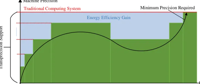
Transprecision Computing is undoubtedly tied to the research area known as approximate computing but it also goes beyond the state-of-the-art and evolves it, as it controls approximation both at a finer grain (see Figure 1) and doesn’t imply reduced

precision at application level, despite allowing the exploitation and softening of application-level precision requirements for extra benefits (Malossi, et al., 2018).

(13)

Machine Precision

Computation Progress Minimum Precision Required Traditional Computing System

Energy Efficiency Gain

T ra ns pr ec is ion S upp or t

Figure 1: Discrete precision approximation in a time interval

2.2 OPRECOMP

Open Transprecision Computing (OPRECOMP) is a 4-years research project funded

under the EU Framework Horizon 2020, coordinated by IBM and backed by a consortium of 10 among universities and companies that hold different key roles and focus on different tasks (OPRECOMP, 2019). The project goal is to build the foundation for computing based on transprecision analytics. The driving principle behind the approach is that almost any application involves a large number of intermediate calculations, whose accuracy is irrelevant to the final user, who is interested only in the reliability and validity of the final result. OPRECOMP wants to provide full support to Transprecision Computing through the development of a transprecision framework spanning all layers of computing systems, from devices, architecture and circuits design to software environment, tools, algorithms and data structures, along with the mathematical theory and physical foundations of the ideas (OPRECOMP, 2019).

(14)

6

Transprecision Framework

Open Transprecision Computing

Algorithms Architecture & Circuit Design Software Environment & Tools

Physical foundations & Mathematical Theory

Disruptive Technology Modeling & Exploration

Figure 2: The complete coverage of the framework (Malossi, et al., 2018)

OPRECOMP is ultimately oriented toward developing and affirming a radically new computing paradigm. An ecosystem inspired by nature and human intelligence, designed to spend just the right amount of energy required for performing any particular operation. While high precision arithmetic will still be mandatory for financial applications, others such as data-mining or human-consuming applications will have the ability to adopt – or in some cases even embrace – less precise arithmetic despite the errors produced by underpowered or new emerging circuits technologies (OPRECOMP, 2019).

2.3 FlexFloat

There are many state-of-the-art tools and libraries available to developers and researchers which allow emulating arbitrary floating-point types of which MPFR (The GNU MPFR Library, 2019) or SoftFloat (Hauser, 2019) are among the most notables. While coupling floating-point emulation with precision tuning is the right approach to target both precision reduction in applications being developed for existing hardware (and thus IEEE floating-point formats compliant) and the specification of formats for new hardware being designed, these libraries are not designed for this purpose (Tagliavini, Marongiu, & Benini, 2018).

(15)

FlexFloat is an open-source software library2_{specifically designed to aid and} improve the development of transprecision applications. Unlike those abovementioned, the FlexFloat library:

1. Uses an emulation methodology that leverages native host platform types to significantly reduce the time required to emulate custom types;

2. Enables accurate emulation of formats with arbitrary bit-width of mantissa and exponent fields;

3. Requires no modification at all to support custom types;

4. Provides advanced statistics on program variables that can be used by optimization models to enhance the solution and/or decrease the search time (Tagliavini, Marongiu, & Benini, 2018).

Since FlexFloat is not the main focus of this paper, the technical details regarding internal implementations of custom types and other features will be omitted from this paper. However, in order to better understand the objectives of what is going to be covered in chapter 5, it is important to clarify how this library is structured to represent floating-point data types and operations. FlexFloat internally represents floating-floating-point types as a data structure composed of two unsigned integers (e, m) and a floating-point field (v) so that 𝑒 + 𝑚 = 𝑙𝑒𝑛(𝑣) − 1, where len(v) is expressed in bits. v is also known as backend

value and it’s the system standard memory block that actually stores the value. The format

of a type expressed by this data structure follows the conventions of the IEEE standard: 1 bit for the sign, e bits for the exponent and m bits for the mantissa. Its value can be computed using the formula −1𝑏𝑚+𝑒 _{× 0. (𝑏}

𝑚−1… 𝑏0)2× 2(𝑏𝑚+𝑒…𝑏𝑚)2−𝑏𝑖𝑎𝑠, where 𝑏𝑖𝑎𝑠 = 2𝑒−1_{− 1 (Tagliavini, Marongiu, & Benini, 2018).}

m+e m 0

e m

sign

Figure 3: FlexFloat internal representation of a floating-point type

(16)

8

It’s also important to know that exactly like in classic computation operations between different precision variables cannot be executed without a cast. In FlexFloat this cast is considered exactly like another temporary variable that will store a value just for the duration of the computation and it is part of all the variables that are considered when fine-tuning the precision of intermediate computations:

1. var1 = var2 + var3 --> var1 = var4(var2) + var4(var3)

In this example, another temporary variable (var4) is added to the computation involving three variables. Just like the other three, var4’s precision can be tweaked before compile time.

In order to test the capabilities of this library, ten programs from different application domains were selected, constituting a benchmark suite that has been used (partially) to also test the performance of this project. Since all floating-point variables in the benchmarks are implemented as double types, all experiments presented in this paper have used a FlexFloat testing unit with a 64-bits backend (using standard hardware architectures).

(17)

Active Learning

3 Active Learning

When it comes to using a machine learning approach to a problem there are two initial issues to address:

• Acquire enough useful data for both training and testing;

• The type of learning task to use, chosen among supervised, unsupervised or a hybrid between the two (reinforcement learning won’t be considered in this paper).

There are cases where it is really easy to both obtain and label enough data to build robust training and test sets and therefore where a supervised learning approach works best. There are also opposite cases where labeling data turns out to be so difficult, expensive or time-consuming that a supervised approach would just fail. Of course, it is always possible to use an unsupervised learning approach but, depending on the problem, it may not be a useful path to follow. It is in these last cases that Active Learning (or “Query Learning”, in short AL) has empirically proven to be effective, although not without drawbacks.

3.1 Concept

The key hypothesis in Active Learning is that if the learning algorithm is allowed to choose the data from which it learns it will perform better with less training. It is a form of supervised learning applied to those cases where there are difficulties in acquiring labeled data: Active learning systems attempt to overcome this labeling bottleneck by asking queries in the form of unlabeled instances to be labeled by an oracle, usually a human annotator or an automatic tool (Settles, 2009).

Let’s consider a classification problem with a target dataset 𝒵 = {(𝑥1, 𝑦1), … , (𝑥𝑁, 𝑦𝑁)} where 𝑥𝑖 is a D-dimensional feature vector and 𝑦𝑖 is its

(18)

discrete-Active Learning

10

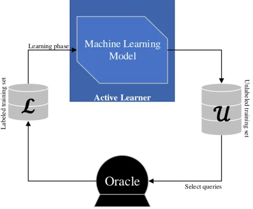
valued label (that could be unknown), the standard Active Learning procedure (also known as a pool-based Active Learning) can be unfolded as follows:

1. The algorithm starts with a small labeled training dataset ℒ ⊂ 𝒵 and a large pool of unlabeled data 𝒰 = 𝒵 − ℒ ;

2. A classifier is trained using ℒ;

3. A query selection procedure picks an instance 𝑥∗ ∈ 𝒰 to be labeled; 4. 𝑥∗ is given a label 𝑦∗ by an oracle and both 𝒰 and ℒ are updated;

5. Repeat from (2) until the desired accuracy is achieved or the number of iterations has reached a predefined limit (Konyushkova & Sznitman, 2017).

Machine Learning

Model

Oracle

L a be le d t ra ini ng s et U_nl abe le d t ra ini ng s e t Learning phase Select queries Active Learner

Figure 4: Pool-based active learning cycle

The pool-based Active Learning is the most commonly used sampling method, applied to fields like text, image or video classification, speech recognition, and information extraction, but there are other methods worth mentioning:

(19)

Active Learning

• Membership Query Synthesis, where the learner may request labels for any unlabeled instance in the input space. In this setting, the active learner generates synthetic instances to be labeled instead of selecting among a pool of samples. This method has been proven to reduce the predictive error rate more quickly than a comparable pool-based sampling. There is the possibility that the generated queries may be humanly unintelligible, making this approach inapplicable whenever the oracle is a human annotator (e.g. queries generating an artificial hybrid word with no meaning when attempting to recognize handwritten words). • Stream-Based Selective Sampling, a method generally used when obtaining

unlabeled instances is free or relatively cheap. In this case, the query can be sampled from the actual distribution and then the learner can decide whether or not to request its label (Kyu Hyun, 2017).

Once the sampling method has been established, the next step is to find a heuristic to select (or generate) the most informative unlabeled instances. There are several learning criteria that have been studied in literature, where the most noticeable are:

• Uncertainty Sampling, where the active learner will select a data point among those it is the least certain about (i.e. in a binary classification problem the one closest to 0.5 confidence);

• Query by Committee Algorithm, where a “committee” of machine learning models trained with the same label instance is established. The task of each model of the committee is to vote on labeling unlabeled instances, and the one the committee disagree the most about is selected as the next query. These two criteria, although commonly used in many Active Learning Applications, haven’t been applied in this specific instance and therefore won’t be discussed further. For a more detailed explanation refer to “Explaining Active Learning Queries” by Kyn Hyun Chang, 2017.

(20)

Active Learning

(21)

Mathematical Programming

4 Mathematical Programming

Also known as Mathematical Optimization, Mathematical Programming (in short MP) is – in its broadest sense – the selection of the best element from a set of alternatives, following a certain criterion. In the most common case, an optimization problem consists in minimizing or maximizing a target function by assigning values to input variables from an allowed set which gives the best result with regard to the target function. A more rigorous definition can be expressed as follows:

Let 𝐹 ⊆ ℝ𝑛 be the set of feasible solutions (corresponding to all vectors 𝑥 satisfying the

constraints of the problem), and 𝑑: 𝐹 → ℝ a function associating a real value to each

feasible point of 𝐹. The couple (𝐹, 𝑑) defines the optimization problem that consists of

finding a point 𝑓 ∈ 𝐹 (global optimum) such that 𝑑(𝑓) ≤ 𝑑(𝑦) ∀𝑦 ∈ 𝐹.

(Martello, 2014) The short notation to express an optimization problem given a target function 𝑑 is

min 𝑥∈𝐹 𝑑(𝑥) or

arg min 𝑥∈𝐹 𝑑(𝑥)

if the focus is the value of 𝑥 that minimizes 𝑑 rather than 𝑑(𝑥) itself.

MP is a wide field of study spanning many different approaches for different scenarios, such as Convex Programming (in turn, a broader category which includes Linear programming), Integer Programming, Non-linear Programming, Combinatorial Optimization, Constraint Optimization, and many others. In the scenario examined by this paper, the nature of the decision variables (discrete-valued) and constraints lead to the use of Mixed Integer Programming techniques. These techniques involve using linear or quadratic programming relaxations to compute bounds on the value of the optimal solution. They also use linear programming and other techniques to compute linear

(22)

14

constraints that cut off possible solutions that violate the discreteness constraints (IBM, 2019).

4.1 CPLEX and DOcplex

CPLEX is a high-performance mathematical programming solver developed by IBM. Originally the first linear optimizer commercially available written in C (its name comes from the union of C and simplex), CPLEX has evolved over timeand now implements mixed integer programming and quadratic programming (IBM, 2019).

Part of the CPLEX environment is the Decision Optimization CPLEX Modeling library for Python (in short DOcplex), a wrapper for the C solver callable using the Python API. It allows solving optimization problems on Cloud service or on the local machine. Fully configurable, it is composed of 2 modules:

• Mathematical Programming Modeling for Python using docplex.mp3 (DOcplex.MP);

• Constraint Programming Modeling for Python using docplex.cp4 (DOcplex.CP) (IBM, 2019).

4.2 Empirical Model Learning

Empirical Model Learning (in short EML) is a technique to enable Combinatorial Optimization and decision making over complex real-world systems. The method is based on the principle of using a Machine Learning model to approximate the behavior of a system that is hard to model by conventional means. The result is an Empirical Model (hence the name) to embed into a Combinatorial Optimization model (Milano & Lombardi, Empirical Model Learning | Embedding Machine Learning Models in Optimization, 2019).

3_{The documentation of this module is available at} https://ibmdecisionoptimization.github.io/docplex-doc/mp/refman.html

4_{The documentation of this module is available at} https://ibmdecisionoptimization.github.io/docplex-doc/cp/refman.html

(23)

In EML the problems of interests are usually defined over high-complexity systems, typically structured as follows:

min 𝑓(𝑥, 𝑧) so that

𝑔𝑗(𝑥, 𝑧) ∀𝑗 ∈ 𝐽, 𝑧 = ℎ(𝑥), 𝑥_𝑖 ∈ 𝐷 ∀𝑥_𝑖 ∈ 𝑥

where 𝑥 is a vector of decision variables 𝑥_𝑖 with domain 𝐷_𝑖 (with no special assumptions on 𝐷𝑖) and 𝑧 is a vector of observables related to the target system. 𝑔𝑗(𝑥, 𝑧) represents a series of logical predicates corresponding to classical inequalities from Mathematical Programming or to combinatorial restrictions. The ℎ(𝑥) function models the complex behavior of the system and specifies how the observables 𝑧 depend on the decision variables: it corresponds to the encoding of the Empirical Model obtained via Machine Learning (Milano, Lombardi, & Bartolini, Empirical Decision Model Learning, 2017).

Embedding an Empirical Model into an optimization model requires encoding the Empirical Model in terms of variable and constraints and therefore exploit the underlying optimization approach to boost the search progress, e.g. via bound computation or constraint propagation. Although the EML Python library5_{(developed by the University} of Bologna) had a major role in the development of this project it will not be discussed further, and its technical details are left to the reader to explore.

(24)

(25)

Project and objectives

5 Project and objectives

This paper will cover some experiments conducted by the University of Bologna as part of the OPRECOMP research project. These experiments aim to develop a reliable decision-making system in the field of transprecision computing by applying a hybrid approach between active learning and mathematical programming. The main goal is to achieve comparable results to those achieved by state-of-the-art tools and methodologies while drastically reducing the execution time. This paper covers the results and experiments conducted by means of a Python script executed locally derived from the work by Borghesi Andrea.

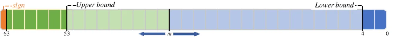
A program using n FlexFloat variables (also counting the temporary ones) requires that each of these variable be set to the lowest precision possible given a maximum tolerated error e on the final result. As stated in chapter 2.3, the backend of each variable is a native double type and thus a 64-bit long value. Considering 1 bit for the sign, there are 63 bits to assign to either the exponent or the mantissa. It has been arbitrarily decided to leave a limit of minimum 10 bits for the exponent and 4 bits for the mantissa, thus effectively limiting the length of the latter to the interval [4, 53].

63 m 0

sign

4 53

Upper bound Lower bound

Figure 5: Visualization of the length limits of the mantissa on a 64-bits long backend

The target decision-making system being designed is composed of two models: an optimization model functioning as the main solver and a machine learning model predicting the error on the final result of the system undergoing study, embedded into the optimization model via the EML library.

(26)

18

5.1 Optimization Model

In order to enforce a proportional relationship between precision and results, the mantissa’s bit-lengths (m in FlexFloat’s floating-point data type) were chosen as decision variables in the optimization model. Let’s then consider the vector 𝑐 of all 𝑚𝑖 values of each 𝑖th variable in a target program (from now on this vector will be referred to as

configuration). We can express the model as follows:

argmin ∑ 𝑐_𝑖 𝑖=1…𝑛 with

• 𝑧 = ℎ(𝑐), where ℎ(𝑐) is the active learning model • 𝑐_𝑖 ∈ [4 … 53], 𝑖 = 1 … 𝑛

• 𝑧 ≤ 𝑒, where 𝑒 is the target error.

It’s important to specify that generally 0 < 𝑒 ≪ 1 and as such it tends to assume values that are difficult to use for exact comparisons on a machine. To account for this issue, the model has been modified to this formula:

• 𝑧 = ℎ(𝑐), where ℎ(𝑐) is the machine learning model • 𝑐𝑖 ∈ [4 … 53], 𝑖 = 1 … 𝑛

• 𝑧 ≥ − log(𝑒), where 𝑒 is the target error.

The choice was guided by the fact that errors expressed as negative orders of magnitude 10−m _{can also be expressed as − log(10}−m_{) = 𝑚. This new formulation inverts the error} constraint, since higher 𝑚 values correspond to more negative orders of magnitude and thus to smaller errors, but also widens the interval of the error value ensuring both better precision on the comparisons and a more ergonomic way to pass the target error as a parameter.

(27)

This base model discussed up to this point, although correct, has been expanded and refined during development to overcome some implementation and performance issues that arose while undergoing testing (see sub-chapters 5.2, 5.3 and 5.4).

5.2 Machine Learning Model and Active Learning

The function binding variable precision and final error is complex and impossible to express analytically. This is why it was impractical to try expressing it through a combination of constraints and expressions directly in the optimization model and why it has been chosen to instead express them through a Machine Learning model. In this scenario, EML turned out to be necessary for successfully blend both the optimization and the machine learning models together and allow the usage of the best of both worlds.

Although the obvious requirement of using a regressor to predict the error (in logarithmic form) given a configuration, the Active Learning phase actually involves the usage of two different Machine Learning models: a neural network used as a regressor and a decision tree used as a binary classifier. The first is used as intended and is embedded into the optimization model as the ℎ function, while the latter is used as an additional tool to discard widely inaccurate solutions. It is also embedded into the optimization model as well and forces it to discard all solutions which it classifies as configurations with an error higher than a certain threshold, hence giving to the optimization model some knowledge about how variables impact the final error. The optimization model with the addition of the classifier can be expressed as the following:

• 𝑧_𝑟 = ℎ_𝑟(𝑐), where ℎ_𝑟(𝑐) is the machine learning model of the regressor • 𝑧𝑐 = ℎ𝑐(𝑐), where ℎ𝑐(𝑐) is the machine learning model of the classifier • 𝑐_𝑖 ∈ [4 … 53], 𝑖 = 1 … 𝑛

• 𝑧_𝑟 ≥ − log(𝑒), where 𝑒 is the target error • 𝑧_𝑐 < 0.5.

(28)

20

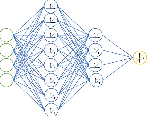
The structure of the regressor depends on the number of variables in the program and its input is the configuration. It is composed of an input layer, two dense hidden layers and a fully connected output layer composed of a single neuron with a linear activation function. The first hidden layer is composed of twice the number of features (which at the time of writing this paper corresponds to the number of variables 𝑛) neurons while the second is composed of exactly 𝑛 neurons. Both the hidden layers use a rectifier6_activation function.

Figure 6: Regressor network for a 4 variables configuration

The structure changes with programs that have high number of variables, in which case the first hidden layer is divided into two distinct fully-connected layers with 𝑛 2⁄ and 𝑛 4⁄ neurons repectively. Both the architectures are the result of empirical evaluations, but it’s extremely probable they are not the best choice available. There are studies being conducted to determine if AutoML techniques7 could be applied to this problem to improve the network architecture.

6_{A REctified Linear Unit (relu) is a unit using the rectifier function 𝑓(𝑥) = max(0, 𝑥) = 𝑥}+_.

7_{AutoML stands for automated machine learning and refers to a series of techniques to automate the whole} machine learning pipeline, from data manipulation to the training of the model (Xin, Zhao, & Chu, 2019).

(29)

Given a program of 𝑛 variables, there are (53 − 3)𝑛 = 50𝑛 different possible configurations. It means that to build a training set big enough to obtain a reliable Machine Learning model requires an exponentially increasing time with 𝑛. The Active Learning approach aims to achieve comparable results by starting with a very limited number of training entries (1000 in each experiment) and refining the ML model with the aid of the optimization model. The refinement process can be described as a variation of a Membership Query Synthesis with an Uncertainty Sampling heuristic naturally obtained through the relation between the regressor and the optimization model: when tasked to find a solution, the MP model uses the regressor to synthesize a configuration, which is then used to run the program and verify its error. If the solution returned by the MP model happens to be unfeasible it means that the regressor made a wrong prediction and thus that specific configuration is one the regressor is uncertain about. Using it to retrain the regressor could potentially improve its accuracy for the next attempt.

5.3 Benchmarks and Variables Graph

The same benchmark suite build for FlexFloat was used to test the system. The suite’s programs represent common algebraical and mathematical operations widely used in the world of scientific and engineering computations. Some of them couldn’t be used for lack of data and the experiments reported on this paper refer solely to the correlation and convolution operation benchmarks. Before moving on it is important to note that the correlation benchmark, at the time of gathering the data reported in this paper, suffered a malfunction which has been discovered only during later stages of the experiments. The wrong values returned by the benchmark don’t void the data presented here per se but render them incomparable to data coming from a functioning version of the same benchmark, without nullifying the observations and comments in the following chapter.

To accelerate the entire process, a tool was introduced to inject into the MP model some knowledge about the variables of the benchmarks and their relations. For instance, it is legitimate to think that if a variable 𝑉 is assigned to another variable 𝑈, they both should have the same precision or 𝑈 should preferably be more precise than 𝑉, just like it is preferable to assign a float variable to a double and not vice-versa. This tool gathers

(30)

22

all the information regarding how the variables interact with each other in a graph data structure called Variables Graph. It stores relations between variables in case of:

• Two variables that are part of an assignment; • Two variables that are part of the same expression;

• Two variables that are linked by a cast operation (the case of temporary variables); • A variable that is the formal parameter of a function and the other is the

corresponding actual parameter.

From a Variables Graph it is possible to extract some semantic information that helps the MP model prune many configurations from the feasible set. For instance, let’s consider the following assignments:

1. var1 = var2 + var3 2. var5 = var6

As already mentioned in chapter 2.3, they are transformed by FlexFloat into this form:

1. var1 = var4(var2) + var4(var3) 2. var5 = var6

Following the convention of incrementally naming all variables, let’s rename variables as ‘T’ if they’re temporary or ‘V’ otherwise.

1. V1 = T4(V2) + T4(V3) 2. V5 = V6

For both the assignments, if the right-hand side expressions (respectively the variables T4 and V6) aren’t used anywhere else, it would be wasteful to allocate to them more memory than the variable their value is going to ultimately be stored into. Therefore, it can be derived that len(𝑇4) ≤ len(𝑉1) and len(𝑉6) ≤ len(𝑉5). Furthermore, the first expression casts two variables with (potentially) different precision to a temporary variable 𝑇4: since FlexFloat makes the design choice of setting the precision of temporary variables to the minimum of the operands, the same relation len(𝑇4) = min(len(𝑉2), len(𝑉3)) can be enforced as a constraint in the MP model.

(31)

Although useful for limiting the solutions pool size, the Variables Graph may impose constraints that are too strict and end up pruning the optimal solution. Here’s an example using the correlation benchmark:

V1

V0

T4

T6

V2

T5

V3

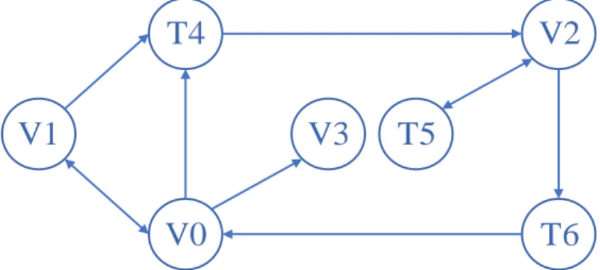
Figure 7: Variables Graph visualization of the correlation benchmark

Figure 7 shows the Variables Graph of the correlation benchmark. Each node represents a variable (names don’t reflect those actually used in the source code of the benchmark) and each arrow represents the relationship between the variables it is connecting. Each

A B _{relationship corresponds to an expression that is traceable to} 1. B = A

hence to the relation len(𝐴) ≤ len(𝐵). The following can be derived from the graph in Figure 7:

• len(𝑉0) ≤ len(𝑉1) and len(𝑉1) ≤ len(𝑉0) → len(𝑉0) = len(𝑉1); • len(𝑉0) ≤ len(𝑉3); • len(𝑉0) ≤ len(𝑇4); • len(𝑉1) ≤ len(𝑇4); • len(𝑉2) ≤ len(𝑇5); • len(𝑉2) ≤ len(𝑇6); • len(𝑇4) ≤ len(𝑉2); • len(𝑇5) ≤ len(𝑉2); • len(𝑇6) ≤ len(𝑉0).

(32)

24

Moreover, the length of a temporary variable (a ‘T’ node) must be equal to the minimum length of all its predecessor nodes (variables):

• len(𝑇4) = min(len(𝑉0), len(𝑉1)) = len(𝑉0) = len(𝑉1); • len(𝑇5) = len(𝑉2);

• len(𝑇6) = len(𝑉2).

Given a generic configuration [𝑉1, 𝑉2, 𝑉3, 𝑇4, 𝑇5, 𝑇6] as the solution of the optimization model, these constraints limit it to all configurations of the form [𝑎, 𝑎, 𝑎, 𝑏, 𝑎, 𝑎, 𝑎] with 𝑎 ≤ 𝑏, constituting about the 0.000016% of the total number of possible configurations. Nevertheless, despite the substantial pruning achieved and the consequent time saving, the optimal solution is also excluded. For instance, the optimal solution for a target error of 10−5 found using state-of-the-art tools is [13, 4, 13, 13, 11, 12, 11] which clearly does not respect the imposed constraints. Another example is found in Appendix I.

With the integration of the Variable Graph-derived constraints, the optimization model can be formalized as follows:

argmin ∑ 𝑐𝑖 𝑖=1…𝑛 with

• 𝑧_𝑟 = ℎ_𝑟(𝑐), where ℎ𝑟(𝑐) is the machine learning model of the regressor • 𝑧_𝑐 = ℎ_𝑐(𝑐), where ℎ_𝑐(𝑐) is the machine learning model of the classifier • 𝑐𝑖 ∈ [4 … 53], 𝑖 = 1 … 𝑛

• 𝑐_𝑗 ≤ 𝑐_𝑘 ∀(𝑐_𝑗, 𝑐_𝑘) ∈ 𝐺, where 𝐺 is the set of all couples of connections 𝑐_𝑘 → 𝑐_𝑗 of the graph

• 𝑐_𝑗 = 𝑐_𝑘 ∀𝑐_𝑗 ∈ 𝑇 and 𝑐_𝑘 ∈ 𝐴_𝑐_𝑗, where 𝑇 is the set of all temporary variables and 𝐴_𝑐_𝑗 is the set of all successors of 𝑐_𝑗 in the graph

• 𝑧_𝑟 ≥ − log(𝑒), where 𝑒 is the target error • 𝑧_𝑐 < 0.5.

(33)

5.4 Structure

The script used to run all the experiments discussed in this paper is a refactored and modified version of the original script. The script has been re-organized and modularized to make it more readable and extendable, in addition to a more complete arguments system to easily tweak all the parameters used during the execution. The version of the project referred to in the next pages can be found in the Git repository at https://github.com/Acciai0/oprecomp_project, with a complete guide to run it.

The new architecture of the script is composed of the following main modules: 1. argsmanaging. This module deals with starting arguments and builds a global

data structure from which to retrieve all initialization values when needed. It is structured so that it is easy to add new labeled parameters or remove unused ones. It automatically handles type conversions from the strings coming from console arguments and all errors that could occur meanwhile. All possible arguments are listed by executing python3.al -help or in the already mentioned Git repository.

2. benchmarks. Module in charge of listing, loading and executing benchmarks. It is used by the argsmanaging module to load all data relative to the given benchmark, such as the construction of the Variables Graph, the number of variables and other information (see the Benchmark class).

3. training. This module manages the construction of a training session, i.e. of a training set and a test set, and the creation and training of both the regressor and the classifier by means of trainer objects specific for the type of model (neural network or decision tree, see RegressorTrainer and ClassifierTrainer classes and the respective sub-classes). It has been built to be easily expandable to also manage other types of regressors or classifiers if needed.

4. optimization. The core of the script. This module is in charge of building the optimization model and iterating until it is solved. It articulates the macro phase of execution described in Figure 8 and exposes functionalities to dump the entire execution to a log JSON file for external purposes (they’ve been used to generate the tables and figures in chapter 6).

(34)

26

5. data_gen. This module contains all functionalities used to manipulate examples for the Active Learning phase and for the Neighborhood Refinements, such as interpolating and generating routines.

6. utils. A utility module which aids the execution by providing utility functions such as I/O routines for reading/writing benchmark-specific files or printing utilities for formatted and colored output (print_n()). It also contains a stopwatch object used to time all critical operations in the program.

This section wants to better define the structure and the control flow of the script and its evolution, starting from the original version and exploring what has been changed in order to obtain the results reported here.

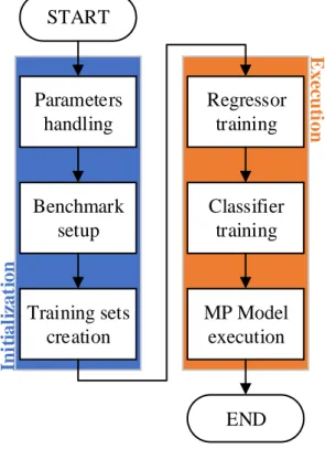
START Parameters handling Benchmark setup Training sets creation Regressor training Classifier training MP Model execution END In it ial iz at ion E xe cu ti on

Figure 8: General control flow of the script

Figure 8 shows the general control flow of both the original and the refactored script: it can be decomposed into two macro phases of initialization and execution where the first phase groups all the operations needed to gather and initialize the required data, while the latter includes all Active Learning applications and optimization steps.

(35)

Parameters handling

Checking of the presence of all mandatory parameters and of their value. In the new script, parameters are labeled and used to tweak not only target error, type of regressor and classifier and the benchmark, but also other internal parameters like the changing rate in the neighbor search (see paragraphs further on) or the delta of orders of magnitude to limit the search into.

Benchmark setup

This phase gathers all data regarding the benchmark specified as a parameter, dynamically getting the total number of variables used in the program, its location on the disk and building its Variables Graph and therefore gathering all the relationships among the variables.

Training sets creation

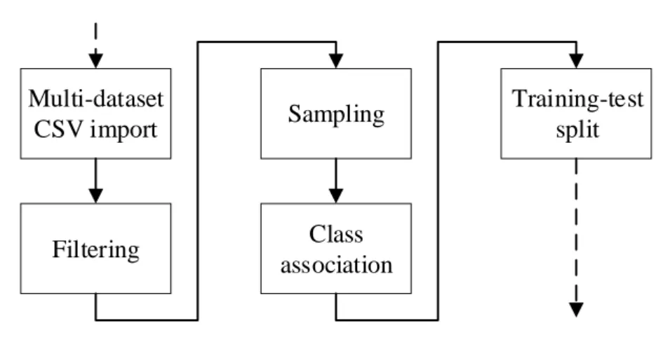
Multi-dataset CSV import Filtering Sampling Class association Training-test split

Figure 9: Training set creation flow diagram

The script works with a series of datasets built differently from one another. All results in this paper have been calculated on the basis of data coming from dataset number zero. First and foremost, the dataset is loaded from the respective CSV file, then filtered to remove any entry with all columns equal to zero. All errors higher than a certain threshold passed as a parameter are clamped to the value of that threshold and a new column containing the logarithm of the errors is also added to the dataset. At this point, the script

(36)

28

randomly samples half of the final number of entries from the dataset and the other half with the following distribution:

• 40% among entries with lower bits sum (these are more critical for training since the regressor has to be as precise as possible when predicting the lower end of the spectrum);

• 30% among entries with low bits sum; • 20% among entries with high bits sum; • 10% among entries with higher bits sum.

For instance, in the case of the correlation benchmark, 40% of the entries will have bits sum between 28 and 114, 30% between 115 and 200, 20% between 201 and 285 and 10% between 286 and 371.

The last steps are the addition of a column specifying the class of each configuration based on the error threshold mentioned prior (errors higher than the threshold are labeled 1, otherwise they’re labeled 0) and the splitting of the resulting dataset into a training set and a test set. The ratio between the test set and the training set is specified via parameter.

Regressor and Classifier training

The training set built in the previous step is used to train both the regressor and the classifier, then they are both tested on the test set to compute some quality metrics (e.g. Mean Squared Error, Mean Absolute Error, Accuracy). The test set is kept until the end of the execution in order to recalculate the metrics after each iteration, while the training set is used again only to retrain the Decision Tree, which cannot be trained using an Active Learning approach.

(37)

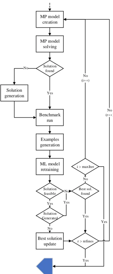
Project and objectives MP model execution Yes MP model creation MP model solving Solution found Benchmark run Solution generation Examples generation ML model retraining Solution feasible Best solution update Best sol. found r > refines i > maxIter No Yes No Yes Yes Yes No (r++) No (i++) No Yes Solution Generated No

(38)

30

Generation of

m neighbors

Filter by Bit sum & graph

Any left Error

interpolation

Error filtering

Any left Best solution

update r > refines Best solution added to pool Bit sum filtering

Any left Error

interpolation

Error filtering

Any left Addition to

the pool r > refines Generation of m neighbors Pool check 1 2

(39)

This macro step is the core of the entire process and the most time-consuming. It is composed of two phases: the first phase of optimization model solving and the second one of local refinement. The first phase is a loop that iterates for a certain number of times or until a feasible solution has been found.

MP model creation

The first step of a single iteration in phase one is the creation of an optimization model. The reason why the same model cannot be used more than once depends on how the EML library embeds a ML model into the MP model. Since what the library does is essentially transforming the structure of a neural network (or decision tree) into the specific representation of the optimization model solver, any retraining carried out on the ML model won’t be transmitted to its embedded representation.

At each iteration, all previous solutions deemed unfeasible are used to define a series of new constraints in order to remove them from the solutions pool and an additional constraint is added to force the solver to find a better solution than the last feasible one it has found (if any). This last constraint is only used for the additional iterations after the first feasible solution has been found, the number of which is specified through a parameter. The final optimization model has the following form:

argmin ∑ 𝑐𝑖 𝑖=1…𝑛 with

• 𝑧𝑟 = ℎ𝑟(𝑐), where ℎ𝑟(𝑐) is the machine learning model of the regressor • 𝑧_𝑐 = ℎ_𝑐(𝑐), where ℎ𝑐(𝑐) is the machine learning model of the classifier • 𝑐𝑖 ∈ [4 … 53], 𝑖 = 1 … 𝑛

• 𝑐𝑗 ≤ 𝑐𝑘 ∀(𝑐𝑗, 𝑐𝑘) ∈ 𝐺, where 𝐺 is the set of all couples of connections 𝑐𝑘 → 𝑐𝑗 of the graph

• 𝑐_𝑗 = 𝑐𝑘 ∀𝑐𝑗 ∈ 𝑇 and 𝑐𝑘 ∈ 𝐴𝑐𝑗, where 𝑇 is the set of all temporary variables and

𝐴𝑐𝑗 is the set of all successors of 𝑐𝑗 in the graph

(40)

32

• 𝑧_𝑟 ≥ − log(𝑒), where 𝑒 is the target error • 𝑧𝑐 < 0.5.

MP model solving

Invocation of the solver and computation of a solution to the optimization problem. If no solution is found (mostly due to the insufficient or poor training of the regressor/classifier) the system generates a random configuration, which serves the purpose of giving some data to work with through the next steps, even without an actual solution. In case the configuration passed to the next steps was generated, it’s not important if it was feasible or not since its role is just to be used to retrain the regressor and, to a lesser extent, the classifier.

Solution generation

If no solution is found during the optimization process (i.e. the solver has concluded that the problem cannot be solved) the most probable cause of the error is a bad training of the regressor, which is temporarily unable to predict low enough values, regardless of the configuration submitted to it. To overcome this error state the regressor needs to be retrained with new entries and because the solver can’t provide a new one, a random configuration is generated. Initially, instead of generating a totally random configuration the script used the previously found solution (feasible or unfeasible) and increased by one unit each value. This choice worked well except if the previous solution was maximized, i.e. [53, … ,53], in which case the new training would have had, in the best scenario, no effect at all.

To avoid this problem, the version used in this paper generates a completely random sequence clamped between [4, … 4] and [53, … ,53], which served its purpose, whilst acknowledging that the solution could be much improved in the future.

(41)

Benchmark run

Whether it is generated or not, the configuration calculated at the previous step is fed to the benchmark and the actual final error is calculated. This step is the most time-consuming, but also the most accurate and its result will be used to check if the solution is feasible or not and as an oracle to retrain the ML models, applying the Active Learning approach automatically.

Examples generation

A single example doesn’t usually affect the training quality in any critical way, therefore it’s important to synthesize a bigger batch of examples to feed to the ML models training session. Using a simple neighborhood search given all the possible values is not applicable in this case, due to the impracticable number of possibilities and thus the memory required (for a benchmark with just seven variables the machine would need 507 ∗ 4 ∗ 7 bytes, which is about 20TB of data). So, to build a batch of examples, the script instead generates new entries using the following algorithm:

1. function GENERATE_NEIGHBOR(configuration, singleChangeProbability, min, max)

2. n = EMPTY_LIST

3. for each value v in configuration 4. p = random value between 0 and 1

5. if p <= singleChangeProbability then

6. delta = int(random sample from a normal distribution

with μ=0 and σ=2)

7. v = v + delta

8. v = CLAMP(v, min, max) 9. APPEND v to n

10. return n 11.

12. function GENERATE_NEIGHBORS(configuration,

singleChangeProbability, min, max) 13. neighbors = EMPTY_LIST

14. neighborsCount = int(1/singleChangeProbability) * 10

15. while not generated neighboursCount neighbors

16. n = GENERATE_NEIGHBOR(configuration, min, max)

17. APPEND n to neighbors

18. return neighbors

(42)

34

Figure 12: Distribution for sampling the deviation of a single value in a configuration

Of course, these entries also need to have an error associated with them. Three different methods have been examined for the task:

• Piecewise linear interpolation. This algorithm has been optimized for data lying on a structured grid while the configurations reported in any dataset are intrinsically arranged in an unstructured manner;

• Radial Base Function interpolation. A powerful mesh-free interpolation algorithm for high-dimensional data. It’s been discarded in favor of the Nearest Neighbor interpolation algorithm.

• Nearest neighbor interpolation. A fast algorithm that assigns to configurations the same error of the nearest neighbor inside the search space. Assuming that among configurations of the same neighborhood the error doesn’t vary too much, the lower precision than the RBF interpolation on the results can be accepted in exchange for a substantial increment of the execution speed.

ML model retraining

The last result and all the examples generated from it (removing duplicates) are used to train the regressor and then they are added to the original training set to retrain the classifier anew (it’s a quick enough process that no incremental training is needed).

(43)

The next step is to check if the given solution is feasible or not: the optimization model returned a configuration on the basis of the regressor’s prediction, which could be wrong, potentially by many orders of magnitudes. In this case, the solution is marked as unfeasible and discarded, while if it turns out to be feasible, it is saved as the current best solution and the algorithm starts another cycle comprising a few more iterations, trying to further improve the solution.

Whether it is because the algorithm cycled for the maximum number of times or it found a feasible solution and finished trying to improve it, in the end, the algorithm will enter the phase two, where it tries to refine the best solution found in the previous phase by executing a neighborhood search for a limited amount of times. This phase has been implemented in two different ways (Figure 11), both with pros and cons. What follows is how the first version works and how it differs from version two.

(44)

36

Generation of m neighbors

The neighborhood search starts by generating more neighbors in the same way as outlined previously, starting from the current best configuration.

Filter by Bit sum/graph

All configurations found in the previous step are filtered to retain only those with a lower bits sum than the current best and that satisfy the constraints given by the Variables Graph. If there isn’t any configuration left after filtering, the loop breaks and the last best solution found is returned.

Error interpolation

To avoid long execution times, this step uses an interpolation method to assign to each configuration an error, instead of calculating it by executing the benchmark. This way the algorithm saves execution time, but it also risks labelling configurations as feasible although that aren’t. To minimize the risk, instead of using the Nearest Neighbor interpolation it uses the Radial Base Function interpolation method.

Error filtering and Best solution update

All configurations with an error higher than the target are discarded and, among those left, the one with the lowest bits sum is chosen as the new best solution.

The second version of phase two works similarly to version one, with a couple of differences:

• Neighbors aren’t filtered using the Variables Graph relationships;

• At each iteration, if a better configuration was found it is added to a pool of solutions;

• At the end of all iterations (or when no more feasible configurations are found), all the configurations in the solutions pool are tested by running the benchmark

(45)

from best to worst and the first solution found to be feasible is returned as the best solution. Compared to version one, this version is a lot more time-consuming, but it can potentially improve the solution found in phase one beyond the constraints enforced by the Variable Graph.

(46)

(47)

Results

6 Results

This chapter reports the results of some experiments ran on different benchmarks and different target errors. It is structured in three parts, each of which focuses on a different part of the execution.

Each experiment will be reported using the following structure:

IT. # CONFIGURATION GENERATED ERROR PREDICTED

0 […, …, …] e1 p1 … … … … … K […, …, …] _✔ ek pk … … … … … N […, …, …] en pn Neighborhood refinements ―

Best solution […, …, …] found in ?s Optimal solution: […, …, …]

Table 1: Experiment report structure

For each optimization iteration, it contains the respective configuration used as a possible solution, as well as an indication of if the given configuration was generated and its error and the prediction of its error coming from the regressor. If there was any configuration coming from a neighborhood refinement, it is listed here, together with the final result, the time spent to find it, and what it is the optimal result. The best solution will be reported at the bottom of the table and, for convenience, it is also highlighted in light blue in the corresponding iteration row. All errors lower than the target are highlighted the same way to help the reader to easily identify those configurations which have been proven to be

(48)

Results

40

feasible. Predicted errors are not highlighted because the regressor, by construction, will always return feasible errors except for generated solutions, which are anyhow ignored as possible solutions. It’s important to keep in mind that the best solution is not, in most cases, the one reported in the last iteration, because after the first solution is found (the first with a highlighted error) the script proceeds for a certain amount of extra iterations trying to find an even better solution. The number of extra iterations can be specified as program parameter and, by default, is set to 4.

6.1 Consistency Tests

The results reported in this section refer to those experiments carried out to test the variance of the results among different executions with the same parameters. The test can only be considered passed if the script can consistently generate comparable solutions at each execution. Here follows an example of five executions of the correlation benchmark, with target error of 10−7_{and no neighborhood refinements.}

IT. # CONFIGURATION GENERATED ERROR PREDICTED

0 [15, 15, 15, 34, 15, 15, 15] 1.324e-07 1.499e-12 1 [16, 16, 16, 16, 16, 16, 16] 1.432e-07 1.467e-12 2 [17, 17, 17, 18, 17, 17, 17] 1.745e-08 1.050e-11 3 [17, 17, 17, 17, 17, 17, 17] 2.402e-08 1.213e-11 4 [38, 36, 44, 4, 33, 23, 23] _✔ 6.479e-01 5.523e-16 5 [42, 18, 33, 29, 15, 49, 45] _✔ 8.494e-10 4.608e-39 6 [51, 51, 10, 37, 38, 42, 16] _✔ 9.999e-01 4.513e-38 Neighborhood refinements ―

Best solution [17, 17, 17, 17, 17, 17, 17] found in 32.063s Optimal solution: [15, 5, 17, 19, 11, 15, 16]

(49)

Results

Table 2: Correlation execution data, target 10-7₍₁₎

0 [12, 12, 12, 23, 12, 12, 12] 1.021e-05 1.100e-12 1 [14, 14, 14, 14, 14, 14, 14] 1.438e-06 2.948e-11 2 [16, 16, 16, 16, 16, 16, 16] 1.432e-07 6.097e-10 3 [18, 18, 18, 18, 18, 18, 18] 6.520e-09 1.195e-08 4 [20, 6, 48, 5, 22, 36, 4] _✔ 4.753e-01 7.641e-03 5 [22, 36, 35, 44, 43, 5, 12] _✔ 2.100e-03 7.715e+18 6 [40, 29, 52, 47, 11, 5, 16] _✔ 2.095e-03 3.381e-32 7 [14, 13, 44, 24, 36, 27, 46] _✔ 2.059e-08 7.448e+00 Neighborhood refinements ―

Table 3: Correlation execution data, target 10-7₍₂₎

0 [29, 41, 29, 36, 4, 19, 40] _✔ 1.595e+09 8.890e-22 1 [46, 28, 14, 29, 32, 18, 33] _✔ 5.725e-07 3.666e-28 2 [13, 13, 21, 42, 11, 40, 11] _✔ 2.722e-06 1.336e-19 3 [4, 4, 4, 4, 4, 4, 4] 1.000e+00 6.709e-08 4 [31, 48, 36, 26, 6, 44, 44] _✔ 8.524e-06 1.875e-66 5 [44, 5, 20, 10, 24, 36, 9] _✔ 3.246e-02 2.133e-23

(50)

Results 42 6 [12, 12, 12, 29, 12, 12, 12] 1.022e-05 2.269e-09 7 [5, 5, 5, 48, 5, 5, 5] 9.999e-01 8.523e-08 8 [15, 15, 15, 15, 15, 15, 15] 4.230e-07 5.769e-09 9 [14, 14, 14, 28, 14, 14, 14] 6.348e-07 7.635e-08 10 [17, 17, 17, 17, 17, 17, 17] 2.402e-08 4.195e-11 11 [8, 8, 35, 21, 11, 20, 43] _✔ 4.851e-05 1.403e-01 12 [43, 49, 44, 11, 12, 47, 12] _✔ 6.021e-03 2.975e-11 13 [28, 5, 20, 38, 47, 8, 41] ✔ 1.594e+09 4.134e-01 14 [26, 41, 27, 45, 11, 33, 19] _✔ 3.984e-08 2.525e-17 Neighborhood refinements ―

Table 4: Correlation execution data, target 10-7₍₃₎

0 [5, 5, 5, 6, 5, 5, 5] 1.000e+00 6.054e-08 1 [29, 46, 11, 16, 11, 21, 32] _✔ 9.999e-01 1.178e-36 2 [13, 13, 13, 13, 13, 13, 13] 8.293e-06 3.030e-09 3 [9, 9, 9, 23, 9, 9, 9] 1.000e+00 2.692e-09 4 [15, 15, 15, 15, 15, 15, 15] 4.230e-07 2.252e-11 5 [17, 17, 17, 23, 17, 17, 17] 1.193e-08 1.703e-12 6 [16, 30, 21, 35, 29, 38, 50] _✔ 1.704e-09 2.047e-07 7 [49, 31, 7, 31, 8, 48, 40] _✔ 9.999e-01 1.005e-14 8 [6, 39, 33, 33, 6, 43, 24] _✔ 8.375e-04 1.912e-01 9 [28, 50, 42, 52, 13, 5, 26] _✔ 2.094e-03 3.971e-11

(51)

Results

Neighborhood refinements ―

Table 5: Correlation execution data, target 10-7₍₄₎

0 [39, 5, 12, 38, 26, 34, 24] _✔ 1.020e-05 1.953e-01 1 [5, 5, 5, 46, 5, 5, 5] 9.999e-01 8.222e-08 2 [12, 12, 12, 49, 12, 12, 12] 1.022e-05 1.318e-11 3 [7, 33, 9, 20, 44, 22, 14] _✔ 9.999e-01 1.127e+03 4 [31, 39, 5, 43, 38, 48, 52] _✔ 9.999e-01 2.506e+03 5 [20, 38, 47, 13, 32, 27, 12] _✔ 5.944e-06 5.054e+02 6 [16, 16, 16, 32, 16, 16, 16] 3.011e-08 8.216e-08 7 [14, 44, 43, 15, 31, 4, 17] _✔ 9.999e-01 1.019e-02 8 [52, 24, 13, 46, 5, 48, 12] _✔ 3.408e-05 6.287e+08 9 [21, 11, 5, 25, 19, 18, 42] _✔ 9.999e-01 3.379e-06 10 [13, 16, 14, 37, 39, 15, 47] _✔ 8.924e-07 8.366e-25 Neighborhood refinements ―