Surface dynamic of copper nitroprusside as a cathode material: observation by XPS and SEM

Alma Mater Studiorum - Università di Bologna

SCHOOL OF SCIENCE

Department of Industrial Chemistry “Toso Montanari”

Master Degree in

Industrial Chemistry

Class LM-71- Science and Technologies in Industrial Chemistry

Surface dynamic of copper nitroprusside as

a cathode material: observation by XPS and

SEM

CANDIDATE

Elisa Musella

SUPERVISOR

Illustrious Professor Marco Giorgetti

CO - SUPERVISOR

Illustrious Professor Reinhard Denecke

Second Session

__________________________________________________________________________________________________________

Academic Year 2016-2017

iv

ABSTRACT

Nowadays, rechargeable Li-ion batteries play an important role in portable consumer devices. The formation of surface films on electrodes in contact with non-aqueous electrolytes in lithium-ion batteries has a deep impact on battery performance. A basic understanding of such films is necessary for the improvement of power sources.

The surface chemistry and morphology of a cathode material, copper nitroprusside, have here been evaluated by X-ray Photoelectron Spectroscopy (XPS) and Scanning Electron Microscopy (SEM), and placed in relation to the performance of the electrodes.

Interface formation between the cathode and carbonate-based electrolytes has been followed and characterised. The variables have been: number of charge/discharge cycles and air contact. The species precipitating on the surface of the cathodes at ambient temperature have been determined to comprise a mixture of organic and inorganic compounds: LiF, LixPFy, LixPOyFz, inorganic and organic carbonates.

v

AKNOWLEDGEMENTS

I wish to express my gratitude for Prof. Giorgetti, my Italian supervisor. This thesis would not have been realised without his encouragement and support, and without him giving me the chance to go to Germany.

I also would like to thank Prof. Denecke for his generosity and kindness and his linguistic and scientific feedback throughout this work, and above all for welcoming me in his research group.

I wish to thank all my co-workers at the Wilhelm-Ostwald-Institut für Physikalische und Theoretische Chemie for many fruitful discussions and friendly atmosphere.

I would like also to thank Angelo Mullaliu for sharing and understanding my scientific and personal dilemmas during this thesis period; it has been invaluable to me.

I must also express my profound gratitude to my friends for providing me with unfailing support throughout my life. You stand with me no matter what. This accomplishment would not have been possible without you.

I take also the opportunity to value all the attempts that my boyfriend Leonardo has done during this hard period abroad for making me feel always his first thought and for putting me always back in the right path in discouragement moments.

Last but not the least, I would like to thank my family: my parents and grandparents for supporting me spiritually throughout writing this thesis and my life in general.

1

INDEX

1. INTRODUCTION: theorical principles ... 10

1.1 X-ray Spectroscopy ... 10

1.1.1 X-ray photoelectron absortion ... 11

1.1.1.1 Energy losses ... 12

1.1.1.2 Quantitative XPS ... 13

1.1.2 Auger spectroscopy ... 14

1.1.3 Scanning Electron Microscope ... 15

1.2 Batteries ... 16

1.2.1 Lithium Ion batteries... 17

1.3 Prussian blue analogues ... 20

1.3.1 Copper nitruprusside ... 22

2. AIM OF THE WORK ... 25

3. EXPERIMENTAL PART ... 27

3.1 XPS measurement ... 27

3.2 SEM measurement... 28

3.3 Sample preparation ... 28

3.5 XPS sample preparation ... 29

3.6 SEM sample preparation ... 29

4. RESULT AND DISCUSSION ... 30

4.1 Measuring the transmussion funtion: 20eV energy pass ... 30

4.1.1 Procedure ... 31

4.1.2 Large area electronics - LAE ... 31

2

4.1.4 Small area electronics - SAE 150 ... 34

4.1.5 Spectrometer with internal scattering ... 35

4.2 XPS Measurement ... 36 4.2.1 Reference ... 36 4.2.2 Charge correction ... 37 4.2.3 Caractherisation ... 40 4.2.3.1 Powders... 40 4.2.3.1.1 AM1 ... 40 4.2.3.1.2 AM4 ... 44 4.2.3.2 Formulated materials ... 45 4.2.3.2.1 AM1_F ... 45 4.2.3.2.2 AM4_F ... 50

4.2.3.3 Formulated materials with electrolyte ... 51

4.2.3.3.1 AM1_E ... 51

4.2.3.3.2 AM4_E ... 54

4.2.3.4 Cycled materials ... 55

4.2.4 Oxidation states of iron and copper ... 56

4.2.4.1 UHV and X-ray aging ... 56

4.2.3.3.1 AM1_F ... 56

4.2.3.3.2 AM4_F ... 59

4.2.3.3.2 General considerations ... 62

4.2.4.2 State of charge and oxidation states ... 62

4.2.5 N 1s evolution ... 63 4.2.5.1 Sputtering ... 67 4.2.6 Depht profiling... 69 4.2.6 Decomposition of electrolyte ... 72 4.2.6 Air modifications ... 75 4.3 SEM Measurement ... 77 5. CONCLUSIONS ... 84 6. BIBLIOGRAPHY ... 86

3

LIST OF TABLES

Table 1: X-rays techniques ... 11

Table 2: Set of sample available ... 25

Table 3: Acquisition parameters for XPS measure ... 28

Table 4: Acquisition parameter ... 31

Table 5: Parameter for LAE lens mode ... 32

Table 6: Quantification of Cu foil calibration sample for LAE lens mode ... 33

Table 7: Parameter for LAX lens mode ... 34

Table 8: Parameter for SAE 150 lens mode ... 34

Table 9: Quantification of Cu foil calibration sample for SAE 150 lens mode ... 35

Table 10: Reference table relative to Na2[Fe(CN)5NO] for assignment of deconvoluted peaks for the active material [41] ... 36

Table 11: Reference table for assignment of deconvoluted peaks for the formulated cathode [42] ... 36

Table 12: Reference table for assignment of deconvoluted peaks for the electrolyte [43]: ... 36

Table 13: Quantification of the specimen for AM1... 43

Table 14: Quantification of the specimen for AM4... 45

Table 15: Quantification for AM1_F ... 49

Table 16: Quantification of AM4_F ... 50

Table 17: Quantification for AM1_E ... 54

Table 18: Quantification for AM4_E ... 55

Table 19: Cycled materials ... 55

Table 20: time aging value for Cu2p peaks of AM1_F ... 57

Table 21: Parameters of fitting curve for Cu+ in AM1_F ... 57

Table 22: time aging value for Fe2p peaks of AM1_F ... 58

Table 23: : Parameters of fitting curve for Cu+ in AM1_F ... 59

Table 24: : time aging value for Cu2p peaks of AM4_F ... 60

Table 25: Parameters of fitting curve for Cu+ in AM4_F ... 60

Table 26: : time aging value for Fe2p peaks of AM4_F ... 61

Table 27: : Parameters of fitting curve for Fe2+ in AM4_F ... 62

Table 28: Oxidation states percentage for cycled samples ... 62

4

Table 30: Depth profiling value for AM17 ... 69

Table 31: Depth profiling value for AM41 ... 71

Table 32: AM1 quantitative analysis ... 77

Table 33: AM4 quantitative analysis ... 78

Table 34: AM1_F quantitative analysis ... 78

Table 35: AM4_F (XPS) quantitative analysis ... 79

Table 36: AM4_F (untreated) quantitative analysis ... 79

5

LIST OF FIGURES

Figure 1: Relationship of probe and analysed beams in surface spectroscopy [3] ... 10

Figure 2: Schematic of x-ray photoelectron spectroscopy process. [4] ... 11

Figure 3: Examples of energy loss phenomena [7] ... 13

Figure 4: Schematic of the Auger electron emission process induced by creation of a K-level electron hole. [4] ... 14

Figure 5: Comparison of the different battery technologies in terms of volumetric and gravimetric energy density. ... 16

Figure 6: Schematic representation of a rocking chair cell ... 17

Figure 7: Sketch of a lithiated graphite composite electrode covered by inhomogeneous SEI. The SEI components shown in darker shades of grey are mainly inorganic while those shown in lighter shades of grey are organic. ... 19

Figure 8: Structure of a metal hexacyano-ferrate ... 21

Figure 9: a) Structure of Cu[Fe(CN)5(NO)]·2H2O b) Structure of Cu[Fe(CN)5(NO)] ... 23

Figure 10: XPS apparatus ... 27

Figure 11: coin cell geometry ... 29

Figure 12: Sample mounted on the sample holder ... 29

Figure 13: calibration curve of Cu+ for AM1_F ... 57

Figure 14: calibration curve of Fe2+ for AM1_F ... 58

Figure 15: calibration curve of Cu+ for AM4_F ... 60

Figure 16: calibration curve of Fe2+ for AM4_F ... 61

Figure 17: Experimental assets of XPS measure ... 63

Figure 18: Tendency for table 28 with differences in focus: ... 66

Figure 19: Depth profile trend for different samples from AM1 set and AM4 set ... 68

Figure 20: Depth profiling trends for AM17 ... 70

Figure 21: Depth profiling trends for AM41 ... 71

Figure 22: Typical SEM micrographs of AM1 . Zoom at a) 300 m and b) 400 m ... 77

Figure 23: Typical SEM micrographs of AM4 . Zoom at a) 300 m and b) 500 m ... 77

Figure 24: Typical SEM micrographs of AM1_F. a) Zoom at a) 90 m and b) 10 m ... 78

Figure 25: Typical SEM micrographs of AM4_F. a) AM4_F after XPS measurement b) AM4_F untreated ... 79

6 Figure 26: Experimental assets of SEM measure ... 80 Figure 27: SEM micrographs of a) AM11 b) AM15 c)AM45 and d)AM47 ... 81

7

LIST OF SPECTRA

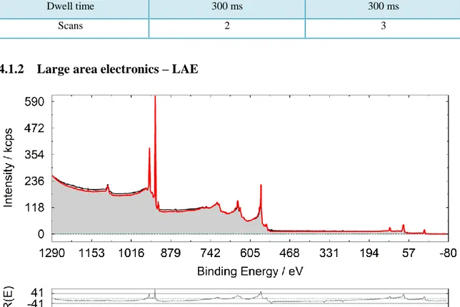
Spectrum 1: Survey Cu foil with LAE lens mode. The red line is the standard spectrum superimposed, the black like in the measured spectrum and the grey part is the area

covered. ... 31

Spectrum 2: fitted Cu 3p signal from Cu foil ... 32

Spectrum 3: fitted Cu 2p3/2 signal from Cu foil ... 33

Spectrum 4: plot of transmission function for three different PE. The T(E) is set to 1 at 1000eV, ... 33

Spectrum 5: Sum curve of F1s from the sample named AM17. The black curve represents the sample itself, without any treatment. The red curve is measured while the flood gun was on and the blue on after the removal of the flood gun. ... 38

Spectrum 6: Sum curve of C1s from the sample named AM43. The black curve represents the sample itself, without any treatment. The red curve is measured while the flood gun was on and the blue on after the removal of the flood gun. ... 38

Spectrum 7: sum curves of N 1s from different AM1 samples. The black set belongs to pristine samples, the red set to cycled ones. The curves were normalized at the major peak to 1 in order to make them comparable on a graph. ... 39

Spectrum 8: survey spectrum of AM1 ... 40

Spectrum 9: C 1s peak of AM1 ... 41

Spectrum 10: O 1s peak of AM1 ... 41

Spectrum 11: N 1s peak of AM1 ... 42

Spectrum 12: Cu 2p peaks of AM1 ... 42

Spectrum 13: Fe 2p peaks of AM1 ... 43

Spectrum 14: C 1s peak of AM4 ... 44

Spectrum 15: O 1s peak of AM4 ... 44

Spectrum 16: survey spectrum of AM1_F... 46

Spectrum 17: C 1s peak of AM1_F ... 46

Spectrum 18: O 1s peak of AM1_F ... 47

Spectrum 19: N 1s peak of AM1_F ... 47

Spectrum 20: F 1s peak of AM1_F... 48

Spectrum 21: Cu 2p peaks of AM1_F ... 48

Spectrum 22: Fe 2p peaks of AM1_F ... 49

8

Spectrum 24: F 1s peak of AM1_E ... 52

Spectrum 25: P 2p peaks of AM1_E ... 52

Spectra 26: Li 1s peak for AM1_E ... 53

Spectrum 27: sum curve of Cu 2p peaks when aging in UHV for AM1_F... 56

Spectrum 28: sum curve of Fe 2p peaks when aging in UHV for AM1_F ... 58

Spectrum 29: sum curve of Cu 2p peaks when aging in UHV for AM4_F... 59

Spectrum 30: sum curve of Fe 2p peaks when aging in UHV for AM4_F ... 61

Spectrum 31: Comparison of N1s peaks of AM44 and AM4_F ... 64

Spectrum 32: N 1s peak of AM41 ... 64

Spectrum 33: all N 1s signals of AM1 set ... 65

Spectrum 34: all N 1s signals of cycled materials ... 65

Spectrum 35: N 1s peaks for sputtering of AM44 ... 67

Spectrum 36: Cu 2p peaks for sputtering of AM17 ... 69

Spectrum 37: Cu 2p peaks for sputtering of AM41. Black curve is the sample untreated (=0min sputtering), the red curve is 5 min sputtering, the blue curve is 8min sputtering and, finally, the green curve is 11 min sputtering... 71

Spectrum 38: fitted F 1s signal for AM14 ... 73

Spectrum 39: fitted Li 1s signal for AM14 ... 73

Spectrum 40: fitted O 1s signal for AM14 ... 74

Spectrum 41: fitted P 2p signal for AM14... 74

Spectrum 42: F 1s signals from AM4 set ... 75

Spectrum 43: Comparison of F 1s peaks coming from AM12 and AM16 ... 76

10

CHAPTER 1: INTRODUCTION

1.1 X-ray spectroscopies

Since the discovery of X-rays by Röntgen [1] over 100 years ago in his laboratory in Würzburg, X-rays have provided a non-destructive characterization of a large variety of materials. X-ray methods cover many techniques based on scattering, emission, and absorption properties of the X-ray radiation. [2]

In general, spectroscopic techniques are used in order to gather chemical information about surfaces. As shown in Fig. 1, a beam is incident on the surface and penetrates to some depth within the surface layer. A second beam exits from the sample and ultimately is analysed by a spectrometer. [3]

Figure 1: Relationship of probe and analysed beams in surface spectroscopy [3]

By varying the nature of the beams in and out, one can generate a large number of surface analytical techniques as seen in the Table 1. [3] The techniques that are shown in bold are the one used in this work.

When probing a surface with any beam, of course one must be concerned with the effect of the probe beam on the surface:

 Photons are the least destructive: in greater than 95% of the cases no decomposition of the surface occurs.

 Electrons are more destructive and the effect varies from insulator to conductors. Electron beams are particularly destructive for organic materials. In addition to chemical effects, electron beams cause serious sample charging for many insulators.

11 Table 1: X-rays techniques

Beam out

Beam in Photons Electrons Ions

Photons Infrared spectroscopy Raman spectroscopy X-Ray Fluorescence Extended X-Ray Absorption Fine Structures X-Ray Photoelectron Spectroscopy UV-Photoelectron Spectroscopy Proton-Induced Auger Electrons Laser Mass Spectrometry Electrons Electron Microprobe Appearance-Potential Spectroscopy Catholuminescence Auger Electron Spectroscopy Low-Energy electron Diffraction Electron Microscopy Electron-Impact Spectroscopy Electron-Induced Ion Desorption Ions Ion Microprobe: X Rays Ion Induced X-Rays

Ion Neutralization Spectroscopy Ion-Induced Auger Electrons Secondary-Ion Mass Spectrometry Low-Energy Ion Scattering Spectroscopy High Energy Ion

Scattering Spectroscopy Ion-Microprobe: Ions

1.1.1. X ray photoelectron spectroscopy

Figure 2: Schematic of x-ray photoelectron spectroscopy process. [4]

X-ray photoelectron spectroscopy (XPS) in a non-destructive technique in which incident photons excite the atoms in the samples to produce electrons. [4]

XPS is based on the photoelectric effect when an incident x-ray causes ejection of an electron from an atom. In this process, an incident x-ray photon of energy h impinges on the atom causing ejection of an electron, usually from a core electron energy level (as

12 shown in Fig. 2). This primary photoelectron is detected in XPS. For the primary electron, which is bound to the atom with binding energy EB (for solids referenced to the Fermi energy), to be detected in XPS, the electron must have sufficient kinetic energy to overcome, in addition to EB, the overall attractive potential of the spectrometer described by its work function SP. Thus, the kinetic energy Ekin of this photoelectron is given by:

𝐸𝑘𝑖𝑛 = ℎ𝜈 − 𝐸𝐵− Φ𝑆𝑃

If the energy of the x-rays and the spectrometer work function are known, the measured kinetic energy can be used to determine the binding energy EB from:

𝐸_𝐵 = ℎ𝜈 − 𝐸_𝑘𝑖𝑛− Φ_𝑆𝑃

This EB is characteristic for each energy level in the element and can be used to determine the element from which the electron originated.

The sensitivity of XPS towards certain elements is dependent on the intrinsic properties of the photoelectron lines observed. The parameter governing the relative intensities of these core-level peaks is the photoionization cross section . This parameter describes the relative efficiency of the photoionization process for each core electron as a function of element atomic number.

XPS is a surface-sensitive technique as opposed to bulk techniques because electrons cannot travel without interaction, so the depth from which the electron information is obtained is limited by “the escape depth” of the photo-emitted electrons. [4] Typical escape depth for XPS with the parameters used in this work is 20 Å. [3]

In this sense, XPS can firstly be applied as a simple qualitative tool to establish the presence or absence of elements on a surface. It is sensitive to all elements except H and He. The typical information that we can gather from an XPS measurement are: [5]

 oxidation state

 bounding information

1.1.1.1 Energy losses

As well as the generation of core photoelectron lines in XPS, certain outgoing photoelectrons undergo characteristic energy losses as they are ejected from the atom, ion or molecule. Such well-defined losses should not be confused with the general cascade of inelastic collisions or secondary electrons that occur once an electron has been ejected and give rise to a step-like background, but involve promotion of electrons within the atom to a higher energy level: the consequential loss of kinetic energy by the

13 photoelectron is observed in the XPS spectrum as a minor peak to the higher binding energy side of the characteristic core level. [6] Such phenomena include shake-up and shake off-satellites.

Figure 3: Examples of energy loss phenomena [7]

Figure 3 shows a schematic to describe the processes involved. Shake-up satellites occur when the outgoing electron interacts with a valence electron and promotes it to a higher energy level. The kinetic energy of the core electron is slightly reduced and consequently appears at slightly higher binding energy within the photoelectron spectrum as a characteristic satellite structure. A related occurrence is that of shake-off in which the valence electron is ejected completely from the atom. [6] Another phenomenon that may happen is multiplet splitting. Multiplet splitting of a photoelectron peak may occur in a compound that has unpaired electrons in the valence band and arises from different spin distributions in the electrons of the band structure. This manifests itself as a core line that appears as a multiplet rather than the expected simple core line structure. [6]

1.1.1.2 Quantitative XPS

XPS spectra also bear a relationship between photo-electron intensity and number of atoms sampled. Quantification of these data can be achieved with a precision to within ca 10%. For a homogeneous sample analysed in a fixed geometry, the relationship between XPS intensity and number of atoms is given by:

𝐼_𝐴= ∫ 𝜎_𝐴𝑛_𝑎𝐾𝐹_ħ𝜔𝑒𝑥𝑝( −𝑧 𝜆_𝐴cos 𝜗)_𝑑𝑧

where IA is the XPS intensity line of the substance A, A is the cross section for excitation of a substance A, nA is the density of the substance A, K is instrument factor

14 (comprehensive of acceptance angle, detection sensitivity, transmission function and illuminated area), Fħ is the photon flux,  is the mean free path for measured line and 𝜗

is the emission angle. [7]

1.1.2. Auger Spectroscopy

Figure 4: Schematic of the Auger electron emission process induced by creation of a K-level electron hole. [4]

An Auger electron spectroscopy (AES) spectrum is always recorded while measuring with XPS. AES is also based on an electron ejection process like XPS, but the electrons that are monitored in AES are secondary electrons. The secondary electrons called Auger electrons arise from a process shown schematically in Figure 4. The process occurs after primary electron emission when such a core-level hole exists. Incident electrons are usually used in AES to stimulate primary electron emission, although incident x-rays can also be used as in XPS. The presence of this core-level electron hole results in electron relaxation from an outer core level or a valence level to fill the core-level hole. When this relaxation occurs, the excess energy that is released stimulates ejection of a secondary or Auger electron from another core or valence electron energy level. The final state of the atom after Auger electron emission is thus doubly ionized; however this final doubly ionized state is more stable than the initial singly ionized state. The energy of the Auger electron is independent of the energy of the incident electron beam (or photon energy) and depends only on the energies of the three electron levels involved in the process. The kinetic energy of the Auger electron is given by the difference in energy between the primarily ionized core level and the level from which the electron comes that fills the

15 core-level vacancy minus the energy that it takes to remove the Auger electron from the singly ionized atom and the spectrometer work function SP. The Auger transition is identified by a three-letter label in which the first letter indicates the core level in which the initial electron vacancy resides, the second letter represents the electron level from which the electron comes that fills the initial vacancy, and the third letter indicates the electron level from which the ejected Auger electron comes. Thus, for a KLL Auger electron

𝐸_{𝑘𝑖𝑛_𝐾𝐿(1)𝐿(2,3)} = 𝐸_𝑘− 𝐸_𝐿(1)− 𝐸_𝐿(2,3)∗ − Φ_𝑆𝑃

where Ekin_KL(1)L(2,3) is the kinetic energy of the Auger electron, Ek is the energy of the K core level, EL(1) is the energy of the electron level from which the electron comes to fill the K-level core vacancy, and E*L(2,3) is the binding energy of the L(2,3) level in the presence of a hole in the L(1) level. Any three subshells within an atom can be involved in the Auger process as long as the final state is significantly more stable than the initial state. [4]

1.1.3. SEM – Scanning electron microscopy

SEM is the most common and well-known electron microscopy method for imaging of surfaces. This technique is based on the interaction of a primary beam of electrons with energy typically in the range of 0.5–40 keV with a surface. This primary electron beam is first demagnified by a condenser lens and then focused onto the sample surface using a series of objective lenses. SEM must be done in vacuum so that the electrons can travel for distances required. Modern SEMs can achieve a lateral resolution of 1.5 nm at a primary electron voltage of only 1.5 keV. [4] In most SEM analyses, secondary electrons created near the position of the impinging primary beam are detected. However, surface images can also be obtained through collection of backscattered primary electrons. SEM can also be used to obtain spectroscopic information by using the photons resulting from relaxation processes (in this case the relaxation process is fluorescence).

Wavelength dispersive x-ray analysis (WDX) is used in high-energy resolution instruments. EDS (Energy dispersive x-ray analysis) or WDX are based on the emission of x-rays with energies characteristic of the atom from which they originate in line of electron emission. Thus, these techniques can be used to provide elemental information about the sample. In the SEM, this process is stimulated by the incident primary beam of electrons. This process is also the basis of essentially the same technique but with higher

16 beam current and performed in a dedicated x-ray spectrometer for bulk analysis, known as electron microprobe analysis (EMA). SEM/EDS typically occurs in a volume of sample larger than that from which backscattered electrons are observed. Thus, SEM/EDS samples the surface to a greater depth than does SEM imaging. Signals typically result from the upper several microns of the near-surface region. Therefore, this technique, similar to electron probe micro analysis (EMA), is a bulk analysis rather than a surface analysis technique. [4]

1.2 Batteries

Development of novel and advanced rechargeable Li-ion batteries is one of the most important challenges of modern electrochemistry. [8] A battery is a device that converts chemical into electrical energy. A battery is composed of several electrochemical cells that are connected in series and/or in parallel in order to provide a certain voltage and capacity. The cell consists of a positive and a negative electrode separated by an electrolyte solution containing dissociated salts, which help ion transfer between the cathode and the anode. Once these electrodes are connected externally, the chemical reactions proceed at both electrodes, thereby liberating electrons and enabling the current to be tapped by the user. Among the various existing technologies (Fig. 5), Li-based batteries - because of their high energy density and design flexibility - currently outperform other systems, accounting for 63% of worldwide sales values in portable batteries. [9]

Figure 5: Comparison of the different battery technologies in terms of volumetric and gravimetric energy density.

17

1.1.1. Lithium Ion Batteries

Lithium cells are made of lithium metal as negative electrode, an active material as positive electrode, and a non-aqueous lithium-ion containing solution which helps ion transfer between the electrodes: the electrode material should undergo a reversible reaction with lithium ions, typically it is reduced during discharge, while oxidized in charge:

discharge

xLi+ + AM (s) + xe− ⇄ LixAM (s) charge

Active material electrodes may have a porous framework that allows the rapid insertion and extraction of lithium ions with generally little lattice strain. Otherwise, a different lithium ion source may be adopted, since the usage of lithium metal can be dangerous. LixAM’ can be opted for negative electrode, whereas the active material acts as a lithium ion sink, in a way that Li-ions are intercalated in both electrodes:

discharge

xLi+ + AM (s) + xe− ⇄ LixAM (s) charge

This strategy is known as rocking chair philosophy [10] (Fig. 6), and was the first attempt to overcome the safety hazards related to Li, as an un-even growth upon Li metal takes place during alternated cycles of discharge/charge. Using two insertion hosts rather than one erase safety, even though a more positive cathode has to be found since the anode has a less negative potential [9].

18 Commercial swing batteries consist of graphitic carbon as negative electrode and lithium cobalt dioxide as cathode. During discharge lithium is reversibly intercalated in the host material and electrons flow in the external circuit to balance the reaction. During charge the non-aqueous electrolyte mediate the transfer of Li-ions in the opposite direction [9]. The other key component of a battery is the electrolyte, which commonly is referred to a solution comprising the salts and solvents. The choice of the electrolyte is crucial, and it is based on criteria that differ depending on whether we are dealing with polymer or liquid-based Li-ion rechargeable batteries. [11]

There are a great number liquid solvents available, with different dielectric constants and viscosity, and it is possible to select specific solvents to favour the ionic conductivity. However, there are only a few Li-based salts or polymers to choose from. [9]

The most common salt used for Li-ion battery is LiPF6. It is usually employed for its ionic conductivity, but it is thermally unstable, decomposing in LiF and PF5 and generating HF if water is present.

P F6− ⇆ P F5 + F −

In terms of cyclability, this means that the battery performance would decline.

The other option might be lithium imide salts, for instance lithium bis(triflouromethane sulfonyl) imide salt, denoted as LiTFSI, which is safer and more stable than LiPF6. LiPF6 has a higher conductivity and even a greater viscosity compared to LiTFSI, due to the PF6

−

anion coordination by solvent molecules. However, under the same conditions, the performances result better for LiTFSI than for LiPF6 [12].

Concerning the liquid solvents, ethylene carbonate (EC) is usually present as solvent in the Li-ion solution, as it forms an electron insulating yet stable ion-conducting layer on the anode, which avoids degradation. This film is called solid electrode interface (SEI) and it is responsible for the stability of Li-ion batteries [9]. However, EC cannot be used alone, as it is solid at room temperature. It is commonly mixed with propylene carbonate (PC) and/or dimethyl carbonate (DMC), the former not compatible with graphitic compounds causing exfoliation (if SEI has not been formed yet) [13], the latter melting at 2°C, so not used alone as well in low temperature applications. Mixing EC with other carbonates makes not only the solvent mixture liquid, but optimal viscosity and ion-conductivity are also achieved.

Carbonates are considered optimal solvents for Li-ion batteries, since they are available at an affordable price, and can dissolve Li-salts enough to achieve a good conductivity,

19 although the electrolyte concentration should not overcome the value of 1-2 mol/L for viscosity issues. [14]

As far as concern electrochemical cells, interfaces play an important role: the electrode/electrolyte interface may be responsible for a poor cycling, as side reactions may occur.

By far, the most common active material used in the negative electrodes is graphite (C6 + xLi+ + xe− ⇆ C6Lix). However, there are a variety of other kinds of carbons which have also been used. As positive electrode mostly transition metal oxides and phosphates have been employed, out of which LiCoO2, LiMn2O4, and LiFePO4 are the most common ones. [15]

During first charge of the Li-ion battery the electrolyte undergoes reduction at the negatively polarized graphite surface. This forms a passive layer comprising of inorganic and organic electrolyte decomposition products as shown in Fig 7. In an ideal case this layer prevents further electrolyte degradation by blocking the electron transport through it while concomitantly allowing Li-ions to pass through during cycling. This essential passive layer has been named solid electrolyte interphase (SEI) [16]. Some solvents such as cyclic alkyl carbonates form effective passive layers that ensure good cycling stability of the negative electrodes. [15]

Figure 7: Sketch of a lithiated graphite composite electrode covered by inhomogeneous SEI. The SEI components shown in darker shades of grey are mainly inorganic while those shown in lighter shades of grey are organic.

All parameter and property of the SEI deeply affects battery performance. The composition, thickness, morphology, and compactness are a only some examples. Irreversible charge “loss” (ICL) in the very first cycle occurs due to solvent reduction and SEI formation and is hence a characteristic of SEI [17]. Damaging processes

20 occurring during storage (self-discharge) also depend on the ability of the SEI to passivate active material surface. [15] Hence, the life of a battery also depends on SEI [18]. SEI may also dissolve and/or evolve during cycling. Thus, effective and stable SEI is mandatory for good cycling life of the battery [19]. It becomes even more important during cycling at high rates and at deeper depth of discharge [20]. However the most important consequence of SEI is on the safety of the battery [21].

Some interface phenomena is occurring also on the cathode side of the cell, even though the validity of the SEI-layer concept is still somewhat tenuous in this “cathode” context. The implication is that Li+ ions must also travel through an additional (solid electrolyte interphase (SEI)-type) layer between cathode and electrolyte – a process which could even prove rate-limiting if the surface species so formed were poor ion-conductors and Li+-ion diffusion through the electrolyte and bulk electrode material were fast [22].

1.3 Blue Prussian Analogues

Transition metal hexacyanoferrates of the general formula AhMk[Fe(CN)6]l ∙ H2O, in which:

 h, k, l, m are stoichiometric numbers,

 A is the alkali metal cation,

 M is transition metal ion,

represent an important class of mixed-valence compounds, of which Prussian blue or iron(III) hexacyanoferrate(II) (with A = K and M = Fe in the above generic formula) is the classical prototype. [23]

Prussian Blue is a ferric ferrocyanide with the formula FeIII4[FeII(CN)6]3 with iron(III) atom coordinated to nitrogen and iron(II) atom coordinated to carbon. [24] It was originally named Berliner blau and it was accidentally synthesized for the first time in 1704 by Heinrinch Diesbach and had applications not only as blue pigment and replacer of the much more expensive lapis lazuli, but also as antidote. It actually consists of an open-framework structure, which was useful for trapping irreversibly thallium (I) ion, which could replace the interstitial potassium ion deriving from the reactants [25]. This feature, known as ion exchange, is nowadays used for trapping caesium-137 from waste streams in the processing of nuclear fuels [23].

21 Prussian blue presents two different form: soluble and insoluble. This distinction is not referring to a real solubility, instead to a tendency to form a colloidal solution or not, due respectively to the absence or presence of vacancies and interstitial cavities. [23]

Prussian blue analogues (PBAs) are bimetallic cyanides with a three-dimensional lattice of repeating units of -NC-Fe-CN-M-NC-, where M denotes a transition metal, generally Mn, Co, Ni, Cu, Zn [25]. As iron is commonly present, these compounds are recognised as hexacyano ferrates, otherwise in case of absence of iron, they are just called hexacyano metallates. Many works have been written about PBAs, for instance regarding electrochemical detection of hydrogen peroxide. [26]

Figure 8: Structure of a metal hexacyano-ferrate

The cyano ligand is like a bridge between Fe and M, linking them in a precise way, the carbon bound to Fe, while the nitrogen to M (Fig.8) , whereas M is a divalent ion. Moreover, iron is usually present as Fe (III) in a low-spin state due to the strong-field ligands. A change in the M oxidation state from (+2) to (+3) provokes a contraction in the cell dimensions and it is compensated by interstitial ions [23]. Both Fe and M can be the redox centers, in a way that the overall capacity should be higher than electrodes with just one metal that can act as centers for a redox reaction. [27]

Through the three-dimensional lattice, Prussian blue analogues are also known for the flexibility due to the stretching of cyano ligands, which have the function of mediating a metal-to-metal charge transfer as well [28]. The C-end has the possibility to remove charge through a π-backbonding, and to place it on the N-end, making possible the

22 interaction between the generally 5 Å distant metals, and giving rise in this way to magnetic and optical properties [29].

Among PBAs properties, also electrochromism is encountered: Co[Fe(CN)6] can change its colour by gaining or loosing electrons, being violet in its oxidized state, while green in the reduced form. Furthermore, the colour of cobalt hexacyanoferrate is attributed not only to the oxidation state of Co, but also to its environment: different cations or presence of water alter its aspect [23].

Regarding the porous structure, the open framework is given by repeated vacancies of the octahedral building unit [M(CN)6]. In these cavities both coordinated and weakly bonded water is present, which can be removed below 100°C without modifying the existing structure [29]. Additionally, these compounds can host both Li- ions due to the large interstices and channels, being so processed for battery use [30].

1.3.1 Copper nitroprusside

Copper ferricyanide Cu[Fe(CN)6] is a a Prussian blue analogue where Fe (II) is replaced by Cu(II). Also in this case, two forms are present, one soluble and one insoluble. The former has a face-centered cubic structure: Fe and Cu ions are octahedrally coordinated to –CN and –NC groups, respectively. The latter has a cubic framework, but 1/4 of the Fe(CN)6 are vacant, so that water molecules can replace the empty nitrogen positions in order to complete the coordination of Cu. Thus, Cu atoms are present in this unit cell with three pseudo-square planar coordinated atoms (CuN4O2) and one octahedrally coordinated Cu atom (CuN6), resulting in an average of CuN4.5O1.5 [27].

Copper hexacyanoferrate can be synthetized using a co-precipitation method: a Cu(II) and a ferricyanide solution are added at the same time under constant stirring, and the product can be collected by filtration. The synthesis takes place at room temperature. Copper nitroprusside has a nitrosyl group replacing one of the cyano ligand. The nitrosyl group does not have the possibility to act like a linking brid, so that the resulting structure has a higher porosity. Moreover, there may be three redox centers, as not only copper and iron can change their oxidation state, but also nitrogen in the nitrosyl group. Actually, the nitrosyl group is a non-innocent ligand and may be present in three different forms within the crystal structure: NO+, NO·, NO−.

23 Nitrosyl group could theoretically undergo a redox reaction, changing meanwhile its geometry:

e- e

-NO+  NO·  NO− Linear  bent  bent

The resulting battery capacity would be increased due to the number of electroactive species, whereas the geometrical modification could be observed by IR spectroscopy, the linear -NO absorbing around 1940-1950 cm−1, the bent form at 1400-1700 cm−1. [31] [32] [33]

The hypothesis of a bending of nitrosyl group may be assisted by the case of sodium nitroprusside Na2[Fe(CN)5(NO)]2∙H2O: according to the published works, sodium nitroprusside has been found in two different structures, one having an isonitrosyl, the other one characterized by a bent -NO [34] [35].

In addition, copper nitroprusside could be present either in the hydrated form with two water molecules per unit formula, or anhydrous.

The hydrated structure is orthorhombic. The iron is coordinated to five cyanide ligands and one nitrosyl, the copper is surrounded by four equatorial cyanides and two axial water molecules. The axial -NO and -CN groups do not act as bridge ligands. Moreover, copper shows axial elongation according to bond lengths calculations due to its d9 electronic configuration and Jahn-Teller distortion (Figure 9a).

24 The anhydrous structure is tetragonal. Copper loses two coordination positions because of elimination of water: for this reason the structure changes and copper coordinates not only to four equatorial cyanides, but also to an axial one, so that the coordination sphere resembles to an elongated pyramid of square base [36] (Figure 9b).

In the anhydrous structure the distance between the oxygen-end of nitrosyl and copper ion is reported to be 2.93 Å [36]: according to the model of hard spheres, this spacing corresponds to the Van der Waals interaction distance, the oxygen radius being 1,52 Å and the copper one 1,40 Å. This interspace suggests no chemical bond between oxygen and copper, and therefore that the nitrosyl group does not bridge the two metals. However, the atoms are close enough to allow a polarization of the -NO electron cloud by the copper ion, which results in an increase of the NO π-backdonation towards iron [36].

Copper nitroprusside has been processed as electrochemical sensor [37]; its use as cathode has been probed by the analytical group in a previous thesis. Electrochemical tests were performed both in coin cells and by using in situ cells: on one hand, coin cells allowed different formulations to be easily tested, on the other operando cycling led a deeper insight to insertion process and both chemical and physical changes. Results of several tests highlighted a modification of the material itself over the first cycles up to a stable active compound able to perform several cycles. Moreover, operando techniques report that structural rearrangement of the material takes place in the very first cycle, as well as electrochemical processes. [38]

25

CHAPTER 2: AIM OF THE WORK

The aim of the work was a better understanding of the surface chemistry of an electrode. For pursuing such purpose, the idea was to investigate the surface through XPS and SEM technique.

Several samples have been prepared and tested electrochemically in a previous work [38]. In the table 2, it is possible to see the complete set of sample analysed in this thesis.

Table 2: Set of sample available

Sample Sample ID Notes

Copper nitroprusside AM1 Powder

Copper nitroprusside AM4 Powder

Copper nitroprusside AM1_F Powder + CB + PTFE + VGCF_H Copper nitroprusside AM4_F Powder + CB + PTFE + VGCF_H Copper nitroprusside AM1_E Pristine – not cycled – only soaked on the

electrolyte

Copper nitroprusside AM4_E Pristine – not cycled – only soaked on the electrolyte

Copper nitroprusside AM11 Charged, beginning of the cycling Copper nitroprusside AM12 Charged, 180 cycles done Copper nitroprusside AM14 Discharged, 143 cycles done Copper nitroprusside AM16 Charged, 1000 cycles done Copper nitroprusside AM17 Discharged, 3 cycles done Copper nitroprusside AM15 Charged, several cycles done Copper nitroprusside AM41 Charged, 64 cycles done Copper nitroprusside AM47 Discharged, several cycles done Copper nitroprusside AM42 Charged, 114 cycles done Copper nitroprusside AM43 Discharged, 51 cycles done Copper nitroprusside AM44 Charged, 22 cycles done Copper nitroprusside AM45 Discharged, beginning of the cycling

Since it has been noticed that a structural rearrangement of the material happens during cycles, there was the interest to follow up the trend of the oxidation states in order to see if a changing on the redox center might cause the observed decrease of capacitance. It has been decided to achieve this kind of knowledge monitoring electrodes in different moments of their life, as shown again in table 2 - notes.

Nevertheless, due to the use of highly energetic photons for excitation of the sample, the risk of radiation damage exists. The highly energetic beam spot may lead to degradation of the SEI (solid electrolyte interphase) components [39] and of the sample itself and may alter their chemical nature. Another problem could also be related to the ambient of

26 the UHV. In order to have a deep insight on this kind of concerns, it has been settled to run some test on two “reference” samples, in order to validate this hypothesis.

Another important feature that has been possible to investigate is the decomposition of the electrolyte during cycle: the electrolyte was LiPF6 in a mixture of carbonates. In particular it has been noticed that the F 1s peak is really useful for such a purpose.

Depth profiling is also been done in order to gain information on the bulk of the electrode.

SEM/EDS measurements have been recorded in order to gain morphological characteristics and to have a comparison in elemental analysis with XPS.

27

CHAPTER 3: EXPERIMENTAL PART

3.1 XPS measurement

The XPS measurements were recorded by VG Escalab 220i-XL spectrometer (figure 10) equipped with a model 220 analyser and a set of six channel electron multipliers with a multidetector dead time of 16 ns. An Al K (h=1486.6 eV) radiation from an Aluminium-Magnesium twin anode source was used for all samples, along with pressures in the analysis chamber of 10-9-10-8 mbar.

Figure 10: XPS apparatus

Some samples were measured while the Flood Gun was on with the purpose of suppressing differential charging on the samples.

Depth profiling of the sample surface can provide useful information on the morphological features of the surface. This can be achieved by Ar+-ion etching (sputtering) of the surface, followed by XPS analysis.

28 Table 3: Acquisition parameters for XPS measure

Parameters of acquisition Survey spectra Detailed spectra

Range -5 – 1305 eV Element depending

Pass Energy 50 eV 20 eV

Step width 0.5 eV 0.1 eV

Dwell time 100 ms 300 ms

Scans 1 4-6

Lens Mode Large area - LAE Large area – LAE

The spectra were analysed and fitted by UNIFIT 2017 (http://home.uni-leipzig.de/unifit/). A Shirley function has been chosen for the fitting of the background. Line synthesis of detailed spectra were conducted using Gaussian-Lorentzian curve.

3.2 SEM measurement

The morphology and the chemical compositions of the samples are investigated by FE-SEM LEO 1525 ZEISS instrument fitted with an EDS detector, working with an acceleration voltage of 20 kV.

3.3 Sample preparation

The analytical group of University of Bologna supplied a set of cathodes (table 2) removed from lithium ion coin cells.

The synthesis of the active material (copper nitroprusside) was based on a co-precipitation method from 20 mM solutions of CuSO4∙5H2O and Na2[Fe(CN)5(NO)]∙2H2O as discussed in a previous work [38]. The cathodes had the following formulation:

 70% w/w active material

 10% w/w PTFE (Teflon)

 10% w/w CB (Carbon Black)

29 Figure 11: coin cell geometry

The coin cell geometry is shown in figure 11. Lithium metal foil was adopted as anode, LiPF6 1M in EC:PC:3DMC without additives as electrolyte.

3.4 XPS sample preparation

All the samples, except of AM16, were exposed to air for a period of at least 1 month. This allowing air species such as CO2, water and similar contaminates the superficies. All the formulated samples were washed with acetone before being fixed on a sample holder with carbon tape as shown in figure 12 and inserted in the XPS machine.

AM16 was treated differently: the coin cell was disassembled in a LABmaster Pro Glove Box and the cathode fixed on the sample holder there and moved to the XPS analyser chamber taking care that no air got in contact with the cathode.

Figure 12: Sample mounted on the sample holder

3.5 SEM sample preparation

All the samples were fixed on a sample holder with carbon tape and inserted in the microscope.

30

CHAPTER 4: RESULTS AND DISCUSSION

In the following chapter all the results will be presented and explained. Firstly will be introduced how the transmission function was recorded in order to gain a more accurate quantitative analysis. After that a characterisation of the material will be reported. The next step is a deeper insight into the various problematic of the materials such as UHV and X ray stability, decomposition of the electrolyte, air contact modifications and the nitrogen issue.

4.1 Measuring the transmission function of the photoelectron

spectrometer

Since all detailed spectra are recorded with 20 eV EP, it was necessary to measure the transmission function in this condition prior to the experiments.

The transmission function T of a particular spectrometer and spectrometer setting determines the fraction of photoelectrons from the sample reaching the detector as a function of their kinetic energies. Although T is a function only of Ekin for older

spectrometers equipped with one x-ray anode and without lenses, for new instruments T depends on four essential setting parameters:

 Kinetic energy Ekin of photoelectrons.

 Pass energy EP.

 Lens mode L.

 X-ray source Q.

giving T(E)  T(E, EP, L, Q). Therefore any investigation of the transmission function T of any spectrometer should account for all the spectrometer settings referred to above. In order to find the unknown transmission function T of any spectrometer, Smith and Seah, Seah and Cumpson et al. recommend the adaptation of measured survey spectra M(E) for X = Au, Ag or Cu on reference spectra S(E) recorded for the Metrology Spectrometer II with MX(E)= TX(E)∙SX(E). The model function consists of seven parameters: T = a0+a1+a22+a33+a44+b1Eb2, where E is the kinetic energy and 𝜀 = (𝐸 − 1000𝑒𝑉)/1000𝑒𝑉. In the energy range 200-1500 eV a transmission function T = a0+b1Eb2 was found to give an appropriate approximation. [40]

31

4.1.1 Procedure

Precautions

 Cu is the reference material that has been chosen

 Polish the sample with first soap and then ultrasonic bath with ethanol

 Insert the sample on XPS

 Survey spectra for detecting C 1s content

 Sputter to get C  0

Analysis

Detail and survey spectra are measured of a Cu foil with 20 eV pass energy with three different lens modes (LAE, LAX, SAE150). The transmission function of each is detected making a comparison with reference spectra. The other acquisition parameters are summarised in table 4.

Table 4: Acquisition parameter

Parameters of acquisition Survey spectra Detailed spectra

Range -5 – 1305 eV Element depending

Step width 1 eV 0.1 eV

Dwell time 300 ms 300 ms

Scans 2 3

4.1.2 Large area electronics – LAE

Spectrum 1: Survey Cu foil with LAE lens mode. The red line is the standard spectrum superimposed, the black like in the measured spectrum and the grey part is the area covered.

32 The survey is fitted with a reference Cu spectrum for comparison. The residuum seems to be quite high, but since a survey spectrum is fitted, it is acceptable.

As mentioned above, the transmission function is described by: T = a0+a1+a22+a33+a44+b1Eb2 The value obtained for this lens mode are summarised in table 5.

Table 5: Parameter for LAE lens mode

Parameters Value a0 -0.3884 a1 0 a2 0 a3 0 a4 0 b1 42.5569 b2 -0.4955

In order to test the resulting transmission function, a relative quantification of two lines in the calibration sample were performed: Cu 3p (spectrum 2) and 2p (spectrum 3) were then recorded and fitted.

33 Spectrum 3: fitted Cu 2p3/2 signal from Cu foil

Orbitals 2p and 3p are fully occupied and considering the sensitivity factors, a ratio of 1:1 is expected.

Table 6: Quantification of Cu foil calibration sample for LAE lens mode

It is considered that in XPS an error approximatively between 5-10% occurs. The result shown in table 6 is on limit of confidence. In spectrum 4 it is possible to observe a comparison between the transmission function measured at three different pass energies.

34 Definitively, if a transmission function at a PE different than the one that has been used for recording the spectra would have been used for quantification, an error on the quantification would have been committed.

4.1.3 Large area XL electronics – LAX

The procedure, the spectra and the results for LAX lens mode are similar to the ones

reported for LAE. In table 7 the parameters of the transmission function T = a0+a1+a22+a33+a44+b1Eb2 are reported.

Table 7: Parameter for LAX lens mode

Parameters Value a0 -1.5942 a1 0 a2 0 a3 0 a4 0 b1 37.0364 b2 -0.3849

4.1.4 Small area electronics – SAE 150

The procedure for SAE 150 lens mode gives back as parameters for the transmission function T = a0+a1+a22+a33+a44+b1Eb2 what is shown in table 8.

Table 8: Parameter for SAE 150 lens mode

Parameters Value a0 1 a1 0 a2 0 a3 0 a4 0 b1 -2191130.3575 b2 -5

35 Table 9: Quantification of Cu foil calibration sample for SAE 150 lens mode

The results are not acceptable. Also freeing all the parameters of the polynomial, it is not possible to achieve a proper result probably due to the internal scattering. This approach cannot be used to measure the 20 eV PE for SAE150 mode, it is necessary to use a different one. This method will not be discussed since it’s not useful to the aim of this work.

4.1.5 Spectrometers with internal scattering

In all spectrometers some internally scattered electrons, Is(E), are detected leading to a measured signal Im(E), given by Im(E) = Ii(E) + Is(E).

Generally the scattered electrons arise at the outer hemisphere in concentric hemispherical analysers and at the mirror electrode in cylindrical mirror analysers.

The problem tends to be worst at low pass energies and, in the extreme case, Is(E) may be greater than Ii(E). Unfortunately, the contribution of Is(E) varies through the spectrum and is not easy to subtract from Im(E). The presence of any significant level of scattering is seen through the ratio Im(E)/ni(E) used to derive T(E) in Eqn T(E)α Im(E)/ni(E) (ni(E) is the spectrum emitted). This ratio gives

𝐼𝑚(𝐸)

𝑛_𝑖(𝐸) ∝ (1 + 𝐼𝑠(𝐸)

𝐼_𝑖(𝐸)) 𝑇(𝐸)

The scattering contribution, Is(E), at energies above and below peaks in an XPS spectrum is very much the same, however the value of it will rise markedly on the low energy side. Thus, whereas Im(E)/ni(E) will change smoothly through this region if Is is very small, a rising step will be observed if Is is significant. If the rise in ni(E) is very large at energies just below a peak, the increase in height of the step will be of the order of Is(E)/Ii(E), where Ii(E) is the spectral intensity at energies just above the peak. [41]

36

4.2 XPS measurement

4.2.1 Reference

For the assignment of the deconvoluted signals of the various peaks, the following references given in Tables 10 to 12 have been used.

Table 10: Reference table relative to Na2[Fe(CN)5NO] for assignment of deconvoluted peaks for the active

material [41]

Peaks Powder

BE Assignment

N 1s 397.2 eV CN

402.5 NO

Fe 2p ½ 722.7 Doublet of Fe(III) complex

Fe 2p 3/2 709.5 Doublet of Fe(III) complex

Table 11: Reference table for assignment of deconvoluted peaks for the formulated cathode [42]

Peaks Cathode BE Assignment C 1s 284.5 eV Graphite 291 + 286 eV PVdF 285.1 Polymeric phase/PEO 286.8 CO 290.0 COOO F 1s 687.6 eV PVdF 684.7 eV LiF 686 eV LiPF6 O 1s 531.6 Carbonates 532.5 CO organic

533.3 semiorganic carbonates (-OLi)

531.5 Li2CO3

Table 12: Reference table for assignment of deconvoluted peaks for the electrolyte [43]:

Assignment Measured binding energy/eV

C 1s F 1s Li 1s O 1s P 2p Carbon black 284.5 - - - - Hydrocarbon 285.3 - - - - LiF - 685.5 56-57 - - Li2CO3 290.2 - 56-57 532 - PEO 286.7 - - 533 - LiPF6 - 688 56-57 - 137.8 LixPFy - 687-688 56-57 - 136.5 LixPOyFz - - 56-57 534 134.5-135

37

For not mentioned signals, NIST XPS database

(https://srdata.nist.gov/xps/main_search_menu.aspx) or the “identify lines” tool of the UNIFIT 2017 have been used.

4.2.2 Charge correction

Analysis of insulating materials by XPS often requires correction of the spectral energy scale due to specimen charging. A widely used method is to align the binding energy scale such that the C 1s line from adventitious carbon contamination is in the range 284.6–285.0 eV. In XPS analysis of polymers, it is common to adjust the energy scale such that the lowest binding energy C 1s contribution (hydrocarbon,–CHx) is aligned to a similar constant value (usually 285.0 or 284.6 eV). [45]

The chemical shifts of functional groups in numerous polymers have been measured in this way. However, with the use of high-resolution XPS instruments, it has been demonstrated that there are small but measurable shifts between chemically similar hydrocarbon functionalities, such as aromatic and aliphatic carbons. In many cases, the alignment of one spectral component to a known binding energy value often relies on complex curve fitting of overlapping features, which can be confidently achieved only when the details of the material structure are known or assumed; for an unknown sample or mixture, this is more difficult. In some cases, the organic structure may not contain any hydrocarbon component. It has been proposed a method using a calibrated electron flood gun to pin the surface potential at a known value. In this procedure, the binding energy of a normally conductive sample is measured in both the grounded configuration and when it is insulated from the spectrometer and floating at the potential of the flooding electrons. The difference in the measured binding energy (grounded versus insulated) is applied to correct the energy scale of an adjacent insulating sample measured under the same conditions. [45]

In some cases only a portion of the sample is insulating with some discrete areas or layers of the sample being conducting or semi-conducting. In these cases a phenomenon known as differential charging can occur. Since the cathode material is a really complex system, as a matter of fact consisting in a mixture of conductive and insulating part, this phenomenon actually occurs. Peaks of F 1s (spectrum 5) and C 1s (spectrum 6) have been chosen as example to show this feature.

38 Spectrum 5: Sum curve of F1s from the sample named AM17. The black curve represents the sample itself, without any treatment. The red curve is measured while the flood gun was on and the blue on after the removal of the flood gun.

Spectrum 6: Sum curve of C1s from the sample named AM43. The black curve represents the sample itself, without any treatment. The red curve is measured while the flood gun was on and the blue on after the removal of the flood gun.

In both cases it’s possible to observe that some parts of the spectra are moving and some other tends to gain intensity keeping the same BE. The simplest and more obvious example is the Teflon area: for F 1s PTFE is located between 688 and 695 eV, for C 1s between 292 and 296 eV. The shift is approximatively 1.5-2 eV. Since some peaks are shifting towards lower binding energy, it’s easy to understand that the intensity gained is due to the overlapping of two or more peaks. Interestingly the removal of the flood gun does not establish the same curve as the untreated one. This is probably due to the fact that more time would have been required in order to go back to the equilibrium position.

39 Since this shift has been established, a charge correction would be needed. However, as it’s not possible to apply an univocal charge correction to the sample, and different peaks under the same signal should be corrected with different values, no charge correction has been done in this work. In fact, the peak related to carbon black in the sample, that can be seen around 284.5 eV in spectrum 6, is in a fixed position and does not move with the flood gun.

Moreover, the binding energies of the active material change drastically between a pristine sample and a cycled one. N 1s peak can be used as example of this feature (spectrum 7).

Spectrum 7: sum curves of N 1s from different AM1 samples. The black set belongs to pristine samples, the red set to cycled ones. The curves were normalized at the major peak to 1 in order to make them comparable on a graph.

The reference shown in table 10 indicates the BE for –CN group at around 397 eV and for –NO at 402, this in good agreement with the red curves. However the pristine materials (black curves) display a shift of around 4 eV toward higher BE.

The idea is that an irreversible rearrangement occurs during the first cycles so that the material becomes somehow more conductive. It’s interesting to notice that small differences are visible also within the two sets. In particular the powder (black set of curves) is the more shifted towards higher energy – this is totally expected since the formulation of the material and the addition of the electrolyte are meant to make the material more conductive and feasible on battery purpose.

It’s in any case quite easy to identify which peak is which. Checking the references from N 1s it’s possible to calculate the shift that occur to any active material and choose among the deconvoluted peaks the one that you are looking for, verifying that the BE

40 gained with this calculated shift is the expected one. These features are valid for both AM1 and AM4 set of samples.

4.2.3 Characterisation

4.2.3.1 Powders

The two sets of samples come from two different powders named AM1 and AM4. The difference between them is that AM1 is anhydrous, with the formula Cu0,8[Fe1,2(CN)5(NO)] * 0,3 H2O and AM4 has hydration water (Cu0,9[Fe1,2(CN)5(NO)] * 1,6 H2O). [38]

4.2.3.1.1 AM1

A survey spectrum has been recorded in order to get elemental information. (spectrum 8)

Spectrum 8: survey spectrum of AM1

All the expected elements are present and no impurities are detected.

Detailed spectra are recorded and fitted to gain information about the specimen and the oxidation states on the sample.

41 Spectrum 9: C 1s peak of AM1

From spectrum 9, C 1s is dominated by the contribution of –CN group and it seems that there is just a small impurity of CO2. The –CN group was identified calculating the shift of N 1s respect to the reference and confirming that the resulted BE was consistent with – CN group in NIST database.

Spectrum 10: O 1s peak of AM1

From spectrum 10, O 1s shows the contribution of three main species: –NO group, –CO and H2O. –NO group and water are expected from the material, –CO instead is an impurity coming from air, it’s probably CO2 considering C 1s peak.

42 Spectrum 11: N 1s peak of AM1

From spectrum 11, N 1s displays the contribution of two expected species: –NO and – CN groups.

Spectrum 12: Cu 2p peaks of AM1

From spectrum 12, Cu 2p indicates the contribution of two main species and a satellite: Cu+ and Cu2+. Only Cu2+ was expected and in fact it’s the dominant species. The presence of Cu+ is probably due to a reduction process that the material goes through while exposed to UHV, process that will be discussed in section 4.2.4.1. Actually, it’s also reported in literature that a certain quantity of Cu+ is present already on the pristine material. [46]

43 Spectrum 13: Fe 2p peaks of AM1

From spectrum 13, Fe 2p shows the contribution of two main species: Fe2+ and Fe3+. Only Fe3+ was expected and in fact it’s the dominant species. The presence of Fe2+ is probably due to same reduction process mentioned above for Cu 2p.

Also a quantitative analysis has been carried on and reported in table 13.

Table 13: Quantification of the specimen for AM1

As far as concern the –CN peak it’s easy to notice that the ratio between C 1s and N 1s is not 1:1, in fact it is 2.7:1. Actually the C 1s is not really reliable in XPS measurement since a lot of impurities can be absorbed on the surface and cannot be resolved with the fitting. I could for example assume that beneath the CN there might also be CO in the C 1s spectrum. The –CO peak instead seems to fit quite well: assuming a CO2 specie, the ratio between C 1s and O 1s is 1:2.1. Also the ratio for –NO between O 1s and N 1s is acceptable, it’s 1.3:1. The ratio between Fe and Cu is 1.1:1, a better ratio respect to 1.5 that was reported in the previous work. [38] Finally, also the ratio between N 1s and Fe

44 2p fits in an acceptable limit, 6.7:1. In this work all the contribution from satellites eventually coming from both iron and copper are not included in the quantification.

4.2.3.1.2 AM4

The survey and detailed spectra of AM4 are quite similar to the one reported for AM1. Only spectra with remarkable differences are reported here.

Spectrum 14: C 1s peak of AM4

From spectrum 14, C 1s is dominated by the contribution of –CN group again but more impurities are present: an aliphatic carbon and a CO species which probably have been absorbed on the surface.

45 From spectrum 15, five species are fitted under the peak of O 1s. Again –NO and water are present, but in this case more –CO signals seem to be absorbed on the surface from air.

Also for AM4 a quantitative analysis has been carried on and reported in table 14.

Table 14: Quantification of the specimen for AM4

As far as concern the –CN peak in this case a better result has been found: the ratio between C 1s and N 1is 1.5:1. The –COx peak is difficult to interpret: considering all the –CO species under the same peak for C 1s and three different contributions for O 1s we gain a ratio of 1:1.33.

The ratio for –NO between O 1s and N 1s is really good, it’s 1.1:1.

The ratio between Fe and Cu is 1.1:1, a better ratio respect to 1.3 that was reported in the previous work. [38]

Finally, also the ratio between N 1s and Fe2p fits in an acceptable limit, 6.8:1.

4.2.3.2 Formulated materials

The two powders, separately, have been mixed in a mortar with carbon black, PTFE and VGCF_H in order to obtain a pellet. These pellets are characterised in this section.

4.2.3.2.1 AM1_F

A survey spectrum has been recorded in order to get elemental information. (spectrum 16).

46 Spectrum 16: survey spectrum of AM1_F

Since PTFE has been added a F 1s peak was expected to appear.

Detailed spectra are recorded and fitted to gain information about the specimen and the oxidation states on the sample.

Spectrum 17: C 1s peak of AM1_F

Spectrum 17 shows a really complex system with 9 different species of carbon. Basically all the –CO and –CH peaks are possible for a sample containing CB and VGCF_H and as far as concern the Teflon area, since PTFE is known for undergoing dehydrofluorination process [47], -CF2- and -CFH- species or similar are likely present, as much as some terminal –CF3.