Influence of refractive index inhomogeneity and interface roughness on the radiating properties of a point source in a layered medium

INFLUENCE OF REFRACTIVE INDEX

INHOMOGENEITY AND INTERFACE

ROUGHNESS ON THE RADIATING

PROPERTIES OF A POINT SOURCE IN A

LAYERED MEDIUM

ENRICO NICHELATTI

ENEA – Unità Tecnica Tecnologie dei Materiali Laboratorio Sviluppo e Realizzazione di Componenti Ottici

Centro Ricerche Casaccia, Roma

AGENZIA NAZIONALE PER LE NUOVE TECNOLOGIE, LʼENERGIA E LO SVILUPPO ECONOMICO SOSTENIBILE

INFLUENCE OF REFRACTIVE INDEX

INHOMOGENEITY AND INTERFACE

ROUGHNESS ON THE RADIATING

PROPERTIES OF A POINT SOURCE IN A

LAYERED MEDIUM

ENEA – Unità Tecnica Tecnologie dei Materiali Laboratorio Sviluppo e Realizzazione di Componenti Ottici

I contenuti tecnico-scientifici dei rapporti tecnici dell'ENEA rispecchiano l'opinione degli autori e non necessariamente quella dell'Agenzia.

The technical and scientific contents of these reports express the opinion of the authors but not necessarily the opinion of ENEA.

I Rapporti tecnici sono scaricabili in formato pdf dal sito web ENEA alla pagina http://www.enea.it/it/produzione-scientifica/rapporti-tecnici

INFLUENCE OF REFRACTIVE INDEX INHOMOGENEITY AND INTERFACE ROUGHNESS ON THE RADIATING PROPERTIES OF A POINT SOURCE IN A LAYERED MEDIUM

ENRICO NICHELATTI

Abstract

A theoretical model is proposed for a point light source – dealt with as a randomly-oriented oscillating dipole – embedded in a layered medium, assuming that the layers composing the medium are affected by inhomogeneity of refractive index and interface roughness. The model puts a method forward for calculating the angular distribution of the light intensity that is radiated in the far field. Several computer simulations of such a point source located in the centre of a 15-layer thin-film Fabry-Pérot filter are shown and the results discussed.

Key words: Layered medium, Multilayer, Point source, Oscillating dipole, Roughness, Index inhomogeneity, Planar

microcavity

INFLUENZA DELLA DISOMOGENEITÀ DELL’INDICE DI RIFRAZIONE E DELLA RUGOSITÀ ALLE INTERFACCE SULLE PROPRIETÀ RADIATIVE DI UNA SORGENTE PUNTIFORME IN UN MEZZO STRIATO

Riassunto

Si propone un modello teorico per una sorgente luminosa puntiforme (trattata come un dipolo oscillante con orientamento casuale) immersa in un mezzo striato, supponendo che gli strati che compongono il mezzo siano affetti da disomogeneità dell’indice di rifrazione e rugosità alle interfacce. Il modello suggerisce un metodo per calcolare la distribuzione angolare d’intensità luminosa che viene irraggiata in campo lontano. Sono mostrate e discusse alcune simulazioni di una sorgente puntiforme di tale tipo posta al centro di un filtro Fabry-Pérot a film sottile formato da 15 strati.

Parole chiave: Mezzo striato, Multistrato, Sorgente puntiforme, Dipolo oscillante, Rugosità, Indice disomogeneo,

Contents

1 Introduction 7

2 Oscillating dipole in an ideal layered medium 7 3 Oscillating dipole in a non-ideal layered medium 10 3.1 Index inhomogeneity . . . 11 3.2 Interface roughness . . . 11 4 Computed examples and discussion 13 4.1 Index inhomogeneity . . . 14 4.2 Interface roughness . . . 16

5 Conclusions 17

A Transformation of solid angle on refraction 19

1

Introduction

The theory of spontaneous emission (SpE) from a point light source—e.g., an atomic or molec-ular system—sandwiched between two close parallel planar mirrors has been developed both in its quantum [1–6] and classical [7–15] approaches, generally leading to equivalent results. The mirrors can be either metallic or distributed Bragg reflectors (DBRs), or of other nature. In this paper a special case of such a setup is considered, that is, a point source located within a thin film bounded by two DBRs.

When the point source is placed within such a layered medium, its SpE properties change in terms of photon angular distribution and intensity; indeed, from a quantum viewpoint, the bound-ary conditions introduced by the embedding medium alter the rate at which vacuum modes stim-ulate SpE from the point system. In the past, analytical emission equations were written both for point [12, 13, 16] and volume sources [17–19] placed within an optical multilayer, so that the angular distribution of SpE could be straightforwardly evaluated.

As far as passive optical properties of multilayers are concerned, non-ideality factors—such as rougness, inhomogeneity, etc.—should be suitably taken into account to theoretically evaluate the reflectance and transmittance coefficients of such devices. In the literature, many works were de-voted to study the influence of roughness [20–30] and index inhomogeneity [31–37] on the optical performances of coatings. Analytical expressions for the direct, specular, diffuse and hemispher-ical intensity coefficients that take into account both index inhomogeneity and roughness, plus thickness non-uniformity (thickness wedge), were put forward [38–41].

The purpose of the present paper is to combine the above results and write equations for SpE of a point source, modelled as a randomly-oriented oscillating dipole, from within a non-ideal multilayer, that is, a layered medium whose layers can be affected by index inhomogeneity and interface roughness. One has to consider that the equations to model light radiation from a dipole located inside a layered medium contain expressions of the reflectance and transmittance coeffi-cients of the surrounding half spaces. Because of that, building a unified model from the previ-ous two—emission from inside a perfect multilayer, reflectance and transmittance of a non-ideal multilayer—could seem trivial at a first glance. This is not the case, as statistical considerations need to be made on the whole expressions of the radiated electric fields rather than on their single components. This concept will be elaborated in section 3.

2

Oscillating dipole in an ideal layered medium

Let us consider a single atomic system sandwiched between two mutually parallel plane mirrors. These mirrors can be single metal layers, DBRs, or even planar multilayers of any kind. The atomic system, being generally much smaller in size than the emission wavelengths, behaves like a point source and can be modelled as if it were a randomly-oriented elementary dipole. As shown later on, the random orientation of the dipole can be dealt with a suitable superposition of basic orientation and polarisation states.

Radiation from an elementary dipole can be described by introducing suitable electric-field source terms [12, 13]. For a dipole that lies horizontally (h) with respect to the medium

layer-n

n

n

z

d

d

d

top external medium

bottom external medium

q q0 q₀ q downward emission upward emission S z = 0

Figure 1.Scheme of a single point source in a multilayer. The point source, S, assumed to be an oscillating

randomly-oriented dipole, is embedded in a medium of refractive index n0and thickness d, and surrounded

by two mutually parallel multilayers. The whole layered structure is placed inside an external medium,

whose top and bottom parts have refractive indices n_↑and n_↓, respectively. The dipole is placed at z = z0,

being z = 0 the centre of the internal layer. The distances of the dipole from the top and bottom mirror are

d_↑and d_↓, respectively, their sum being d_↑+ d_↓= d. The propagation angles, θ0and θ↑↓, are measured with

respect to the normal, both for upwards (↑) and downwards (↓) emission. For simplicity, multiple internal

reflections are not shown in the figure.

ing planes, the source terms are four [12, 13],

Ah,s_↑ ≡ Ah,s_↓ = √ 3 16π, A h,p ↑ ≡ Ah,p↓ = √ 3 16πcos θ0, (2.1) where s and p stand for the polarisation state of the radiated field. The subscript arrows indicate the observation half-space—either upwards (↑) or downwards (↓), see fig. 1. The observation angle θ0 is measured within the central medium (at the dipole position) and with respect to the normal

direction in such a way that its value is set to θ0 = 0 for both normal upward and downward

emission. This angle complies with Snell’s law of refraction [42] when crossing borders of media that have different optical constants. Figure 1 shows a schematic representation of the layered medium with used symbols and conventions. The units of the source terms in eq. (2.1) are those of an electric field, that is, Vm−1in the SI system. If the dipole is vertically (v) oriented, the only non-zero source terms are just two [12, 13],

Av,p_↑ ≡ −Av,p_↓ = √

3

8π sin θ0, (2.2) because the other two are Av,s_↑ = Av,s_↓ = 0.

The above-defined source terms represent the amplitudes of the electric fields radiated by the dipole within the embedding layer—their dependence on the observation distance is neglected for notation simplicity—and are used to evaluate the amplitude of the electric fields that are outcoupled in the far field in the external top (↑) and bottom (↓) half-spaces, respectively, as [12,13]

E_↑↓ = τ_↑↓A↑↓+ ρ↓↑A↓↑

1− ρ_↑ρ_↓ . (2.3) 8

Here and in the following, the double-arrow subscript is adopted as a shorthand form to represent two equations in one: one for the first arrow, the other for the second one. In eq. (2.3), τ_↑ and ρ_↑ (τ_↓ and ρ_↓) are the complex-amplitude transmittance and reflectance, respectively, of the space interval that exists between the dipole and the top (bottom) half-space. Such coefficients depend on both angle and polarisation state [43–45]. Hereafter, the superscripts corresponding to dipole orientation and polarisation state are being applied also to the electric field introduced in eq. (2.3)— e.g., E_↑↓h,sindicates the amplitude of the s-polarised electric field component that is generated by a horizontal dipole having Ah,s_↑↓ as source term. However, they are omitted whenever equations have a general meaning and hold true for any orientation and polarisation state, like eq. (2.3).

Let us assume the external top and bottom half-spaces to have real refractive indices—n_↑ and n_↓, respectively. Let n0 be the refractive index of the medium the dipole is embedded in. In the

following, for simplicity, n0 will be taken to be a real quantity, but the theory can be

straight-forwardly generalised to the case of complex-valued n0. Because E↑↓ can be thought of as the

amplitude of an electric field that is transmitted through the top (bottom) bounding multilayer— the amplitude of such an electric field before transmission being (A_↑↓+ρ_↓↑A_↓↑)(1−ρ_↑ρ_↓)−1—with complex-amplitude transmittance τ_↑↓, the laws of intensity transmission apply [43–45] and the far-field polarised intensity components originated from the dipole, apart from unessential common factors, for s and p polarisation are, respectively,

I_↑↓s = n↑↓cos θ↑↓ cos θ0 E_↑↓s 2, I_↑↓p = n↑↓cos θ0 cos θ_↑↓ E p ↑↓ 2 , (2.4)

which hold true for whatever dipole orientation, either h or v.

The above equations work for plane waves. However, a point source in a homogeneous medium radiates spherical waves, and these are detected in the far field after all the multireflection and transmission processes that are described by the previous equations. A correction to take into ac-count how finite solid angles change on refraction is therefore needed [12,13,46]. Such a correction is derived in appendix A; the result is that a multiplicative factor (n2_↑↓cos θ_↑↓)(n2

0cos θ0)−1 has to

be appended to the intensities in eq. (2.4). Therefore, for a spherical wave, the correct equations are I_↑↓s = n 3 ↑↓cos2θ↑↓ n2 0cos2θ0 E_↑↓s 2, I_↑↓p = n 3 ↑↓ n2 0 E_↑↓p 2. (2.5) These equations, too, are true whatever orientation the dipole oscillates along. Note that if the external and internal media coincide, n_↑↓ = n0, there is no net refraction from inside to outside,

thus eqs. (2.4) and (2.5) coincide and match the general plane-wave rule I = n0|E|2.

Let d be the thickness of the n0-index layer the elementary dipole is embedded in, and let d↑and

d_↓(with d≡ d_↑+ d_↓) be the distances of the dipole from the top and bottom mirrors, respectively, which can be single or multilayer coatings (see fig. 1). By setting z = 0 to coincide with the centre of the layer that contains the dipole and z = z0 to be the position of the dipole itself, one gets

d_↑↓= d

2 ∓ z0, (2.6) where the minus sign corresponds to the upward arrow and the plus sign corresponds to the down-ward one. If the complex-amplitude reflectance and transmittance coefficients of the top and bot-tom mirrors for incidence from inside the dipole layer are indicated as r_↑↓ and t_↑↓, respectively,

one can verify that the following expressions hold

ρ_↑↓= r_↑↓exp[−ikn0(d∓ 2z0) cos θ0

] , (2.7) τ_↑↓= t_↑↓exp [ −ikn0 ( d 2 ∓ z0 ) cos θ0 ] , (2.8) 1− ρ_↑ρ_↓ = 1− r_↑r_↓exp (−i2kn0d cos θ0) , (2.9)

where k is the amplitude of the free-space wavevector, and the assumed phase convention is that exp(−ikz) is a plane wave travelling along the positive direction of the z axis. By using these equations, the far-field intensity corresponding to each orientation of the dipole and polarisation state can be written as [17]

I_↑↓= n

2

↑↓cos θ↑↓

n0cos θ0

F_↑↓A_↑↓+ r_↓↑A_↓↑exp [−ikn0(d± 2z0) cos θ0] 2

, (2.10) where

F_↑↓ = 1 T↑↓

− r↑r↓exp (−i2kn0d cos θ0)

2 (2.11)

is the Airy function, and

T_↑↓s = n↑↓cos θ↑↓ n0cos θ0

ts_↑↓2, T_↑↓p = n↑↓cos θ0 n0cos θ↑↓

tp_↑↓2 (2.12) are the intensity transmittance coefficients of the multilayer mirrors (again, for incidence from inside), with superscripts indicating s and p polarizations [43–45]. Equation (2.10) is a compact form that can be applied to any chosen orientation and polarisation state by selecting the proper A_↑↓, A_↓↑, F_↑↓, and r_↓↑terms.

Finally, for a randomly oriented dipole, the s-polarised and p-polarised far-field outcoupled intensities are found with a superposition of the elementary-orientation components, that is [12, 13], I_↑↓s = 2 3I h,s ↑↓ , I↑↓p = 2 3I h,p ↑↓ + 1 3I v,p ↑↓ , (2.13)

where I_↑↓h,s, I_↑↓h,p, and I_↑↓v,pare evaluated by means of eq. (2.10).

3

Oscillating dipole in a non-ideal layered medium

Now let us consider the case where one or more layers are affected by refractive-index inhomo-geneity or roughness at the interfaces between neighbouring materials—bottom layer/substrate and top layer/ambient medium interfaces included—or both. (Hereafter, for naming convenience, the top and bottom external media of figure 1 will be called ambient and substrate, respectively.) Such deviations from ideality are known to affect the passive properties, like optical transmittance and reflectance, of coatings [38–41]. Therefore, they are also likely to influence the active optical properties of them, for instance, the way an oscillating dipole embedded in a non-ideal multilayer radiates electromagnetic waves into the outer space. As shown in the following, theoretically de-scribing such a behaviour can be approached by suitably adapting tools that had been previously developed to deal with reflectance and transmittance [41].

3.1

Index inhomogeneity

Layers can grow non-homogeneously because, during their deposition, several conditions can vary, the most obvious one being the surface met by molecules or ions that keep arriving onto the grow-ing layer, which is constantly evolvgrow-ing in time. This fact often causes packgrow-ing-density variations during the growing process, hence an even small inhomogeneity of the optical constants of any layer should be not surprising.

Index inhomogeneity is here assumed to be a variation of refractive index occurring along the growth axis of the layer (the z axis in fig. 1), that is, perpendicular to the planes that separate each couple of neighbouring materials in a multilayer. This assumption is quite reasonable due to symmetry in a typical advanced deposition apparatus, wherein planetary-like movements of the substrate are used to maximise uniformity across the deposition surface. Here, only linear inhomogeneity—that is, index gradient—is being considered for the sake of simplicity, but the approach is in principle extendible to higher-order inhomogeneities [38, 39].

Index gradient was previously taken into account to evaluate reflectance and transmittance by means of a perturbation approach [36, 38, 39]. In principle, by analytically solving the scalar wave equation in a medium with linearly-varying index across the propagation direction [47], another kind of approach to reflectance and transmittance would be attainable; however, it would imply the use of special functions and very lengthy mathematical expressions, especially when non-normal angles of incidence and polarisation states have to be considered.

Regardless of how gradient-index is dealt with, the resulting radiated electromagnetic field is formally the same as in eq. (2.3), with the only difference that here the complex-amplitude re-flectance and transmittance coefficients of the surrounding structure, ρ_↑↓and τ_↑↓, properly include the effect of index inhomogeneity according to [41]. For the present paper, the above-mentioned perturbation approach is adopted.

3.2

Interface roughness

Roughness quantifies how much an interface between two materials (or a surface) departs from an ideally smooth plane [25]. The effect of roughness on light crossing an interface or being reflected by it is well known and can be dealt with statistical means [20–30]. The case of more than one rough interfaces in a multilayer has been studied as well [21, 22, 38–41]. The considered rough-ness scale is that one giving rise to light scattering within a small cone from either the direct or the specular axis, that is, root-mean-square (rms) roughness values much smaller than the wave-length of impinging light and correlation wave-lengths of the asperities longer than the wavewave-length are involved [21, 22].

The electric field radiated by a source from within a multilayer affected by roughness should be dealt with by calculating suitable statistical averages. As a matter of fact, because eq. (2.3) is nonlinear in its components, statistical averages must be calculated for the full expression of the radiated electric field—or intensity, depending on which quantity is being investigated—rather than naïvely applying eq. (2.3) after having replaced in it τ_↑↓and ρ_↑↓with their roughness-modified counterparts. The average process can include also the simultaneous effect of index inhomogeneity, if needed, by using the same transfer-matrix approach that was introduced in [41].

Under the hypothesis of statistical ergodicity—assumed here as in [21, 22, 38–41]—one can consider an ideal set of many virtual multilayer samples which are mutually identical in all but in

having slightly misplaced layer boundaries—still smooth and plane, though. These virtual samples constitute a collection of elements the positions of whose coating layer boundaries follow, by hypothesis, Gaussian statistical distributions with standard deviations that are equal to the rms roughness values of the corresponding interfaces in the real specimen. The statistical average of the optical properties of elements is expected to reproduce, by ergodicity, the behaviour of the actual sample.

As previously said, statistical averages on the whole radiated electric fields need to be consid-ered. Thus, the intensity of the axial component (for simplicity, direct and specular components will be both addressed to as ‘axial’ in the following) is

I_↑↓axi = q_↑↓|⟨E_↑↓⟩|2 = q_↑↓ ⟨ τ_↑↓A↑↓+ ρ↓↑A↓↑ 1− ρ_↑ρ_↓ ⟩ 2 , (3.1) where the same order of application of the average and square-modulus operators as in [12, 13, 38, 39] has been used. The complex-amplitude transmittance and reflectance coefficients include, if needed, the effect of index inhomogeneities of the layers. Here, q_↑↓ is equal to the polarisation-dependent coefficient that multiplies the square modulus of the electric field in eq. (2.5) to take into account refraction of solid angles (see appendix A):

q_↑↓s = n 3 ↑↓cos2θ↑↓ n2 0cos2θ0 , qp_↑↓= n 3 ↑↓ n2 0 . (3.2)

Regarding the hemispherical component of the radiated intensity—that is, the axial component along the observation direction plus the diffuse (scattered) radiation, integrated over all the solid angle—it is found by using the same method shown in [40, 41], i.e., by inverting the order of application of the average and square modulus operators,

I_↑↓hem = q_↑↓⟨|E_↑↓|2⟩ = q_↑↓ ⟨  τ↑↓A↑↓₁+ ρ_{− ρ}↓↑A↓↑ ↑ρ↓  2 ⟩ . (3.3)

The meaning of this operator-order inversion is discussed in [40]. Concerning the practical system used to numerically calculate the above averages, for the simulations presented in the following section 4 the Taylor-formula method of [21, 22, 38–40] is applied.

While the axial component is highly directional, the hemispherical component contains the axial component plus a diffuse, incoherent component angularly distributed around the main axis. This diffuse component is formed by light being scattered off-axis by the rough interfaces that are present in the multilayer. Theoretically, the diffuse component can be mathematically isolated by subtracting the axial component from the hemispherical one [40, 41]; on the other hand, evaluating its angular distribution—that essentially depends on features related to roughness and interface structure, such as autocorrelation function, mutual coherence of the interfaces, etc. [21, 22, 48]—is rather a hard task and would deserve a full treatment on its own. Here, only the integrated amount of diffuse radiation will be considered.

Following the same principles of a previously introduced model [40, 41], the diffuse radiation— that is, the integral of the scattered light component over the half-full solid angle—has to be equal to the difference between the hemispherical and the axial component. Because any oscillating

dipole radiates along all the possible directions and polarisation states, the total amount of diffuse radiation must be equal to

∫

I_↑↓dif dΩ_↑↓=∫ (I_↑↓hem− I_↑↓axi) dΩ_↑↓, (3.4) where integration is carried out over the top (↑) and bottom (↓) half-full solid angles. (Note that the left-hand member of the previous equation is actually a double integral, because Idif

↑↓, as said

above, is an integrated quantity itself.) This is the quantity that will be calculated in the following examples (section 4) as far as diffuse intensity is concerned.

Finally, the actual directional status of the radiating dipole—randomly oriented, horizontal, vertical—can be suitably taken into account by applying a proper linear combination of the (h,s), (h,p) and (v,p) elementary components [12,13,40,41]. For instance, for a dipole which is randomly oriented, eq. (2.13) holds true.

4

Computed examples and discussion

To better understand how index inhomogeneity and roughness can affect the radiating properties of a dipole embedded in an optical multilayer, some example computer simulations were done. Their results are here reported and discussed.

The same thin-film structure that was analysed in [41] is considered. The structure is a Fabry-Pérot filter pitched at the wavelength λ = 500 nm in vacuum. It consists of a λ/2 low-index middle layer (the ‘spacer’) sandwiched between two Bragg mirrors, each made of 7 alternating high-index (H) and low-index (L) λ/4 layers, so that the full coating formula is H(LH)32L(HL)3H. The refractive index of the substrate and L layers is nsub= nL= 1.5; that of H layers is nH= 2.5.

Both the ambient medium and the substrate are assumed to be infinitely extended in their respective half-spaces. Reflectance and transmittance spectra of the device can be seen in [41].

Here an oscillating, randomly-oriented dipole is assumed to be placed in the centre of the spacer. That location, if the observation wavelength (in vacuum) coincides with the pitch wavelength λ, is strongly resonant with the cavity and the radiated intensity is larger than if the same dipole were placed in an infinitely extended uniform medium and angularly confined within a narrow numerical aperture. The whole-solid-angle integral of the radiated intensity—which is proportional to the number of radiated photons per unit time—is larger than in a uniform medium as well. This is the well known cavity-enhancement effect.

The theoretical far-field intensity distribution, calculated with the equations of section 2, is plot-ted in fig. 2. As already mentioned, this intensity is larger, especially close to the normal, than the intensity that the same dipole would radiate in a uniform, infinitely extended medium of index nL

(that is, the same index of the layer the dipole is embedded in). There, the radiated intensity would be isotropically distributed with a constant value I_∞ = nL/(4π) (≃ 0.12), much smaller than the

peak values of fig. 2. As far as the whole-solid-angle integral of the radiated intensity is concerned, while one can easily verify that it is equal to nL in the aforementioned infinitely extended uniform

medium of index nL, in the case of the intensity distribution of fig. 2 it can be found by numerical

integration, and is found to be approximately equal to 1.87. This result means that the boundary conditions introduced by the Bragg mirrors boost the radiating properties of the dipole by∼ 25% (1.87/nL ≃ 1.25) with respect to an infinite low-index bulk, and by ∼ 87% with respect to the free

0 2 4 6 8 10 0 10 20 30 40 50 60 70 80 90 100 110 120 130 140 150 160 170 180 190 200 210 220 230 240 250 260 270 280 290 300 310 320 330 340 350 0 2 4 6 8 10 substrate side i n t e n si t y ( a r b . u n i t s) ambient side

Figure 2.Polar plot of the theoretical intensity radiated in the far field by an oscillating, randomly-oriented

dipole radiating from inside a 15-layer thin-film Fabry-Pérot filter. The dipole is located in the very centre of the middle layer. See the text for further details.

4.1

Index inhomogeneity

In line with the study done in [41] for the reflectance and transmittance coefficients of the mul-tilayer structure, a set of four refractive index gradient values is taken into consideration. The absolute amount of index gradient in each layer is set to 15%; it can be either negative or positive depending on the chosen example. Here, like in [41], a negative index gradient means that the refractive index of the layer linearly decreases going from the substrate to the ambient side; a pos-itive inhomogeneity represents the opposite behaviour. The gradient is defined as the ratio of the index difference between the layer extremes to the average index in the layer—this latter coincides with the index value at the centre of the layer for symmetry reasons. In either negative or posi-tive gradient case, the average index of the layer is set to the nominal one that one would have in absence of inhomogeneity. In formulas, the refractive index of a typical linearly-inhomogeneous layer would be

n(z) = ¯n + ∆n

h (z− zc), (4.1) where ¯n is the average (and nominal) index, ∆n is the index maximum span within the layer, h is the layer thickness, and zcis the coordinate of the layer centre. The index gradient is defined as

the ratio ∆n/¯n.

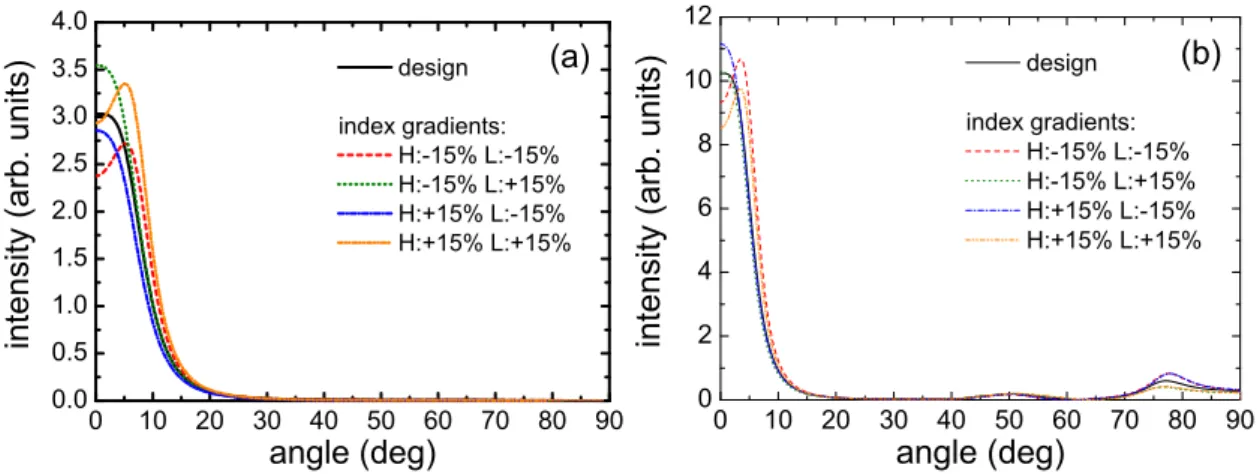
Four cases are here considered. In the first case, all the layers suffer from a negative index gradient, that is, a linear variation of−15%. In the other three cases, the signs of the gradients are alternatively changed for H and L layers, see fig. 3 for a list of the examined cases. This figure shows the far-field intensity in the ambient medium half space and in the substrate. For comparison, plots of the intensities expected in the same multilayer for null inhomogeneities (‘design’ curves), that coincide with those shown in fig. 2, are also shown.

One can notice from fig. 3 that the cases where the inhomogeneity is either positive or negative for all the layers correspond to a dip in the peak of the angular distribution. This fact is in agree-ment with the red-shift by about 1 nm of the pitch wavelength that was found in [41]: indeed, as

0 10 20 30 40 50 60 70 80 90 0.0 0.5 1.0 1.5 2.0 2.5 3.0 3.5 4.0 i n t e n si t y ( a r b . u n i t s) angle (deg) design index gradients: H:-15% L:-15% H:-15% L:+15% H:+15% L:-15% H:+15% L:+15% (a) 0 10 20 30 40 50 60 70 80 90 0 2 4 6 8 10 12 i n t e n si t y ( a r b . u n i t s) angle (deg) design index gradients: H:-15% L:-15% H:-15% L:+15% H:+15% L:-15% H:+15% L:+15% (b)

Figure 3.Theoretical intensities radiated in the far field by an oscillating, randomly-oriented dipole radiating

from inside a 15-layer thin-film Fabry-Pérot filter: (a) ambient side, (b) substrate side. The dipole is located in the very centre of the spacer. The high-index (H) and low-index (L) layers are affected by refractive index

gradient inhomogeneity of±15%. See the text for further details.

grad_H grad_L ∫ Iaxi

↑ dΩ↑ ∫ I↓axidΩ↓ — — 0.3329 1.5363 −15% −15% 0.3746 1.8755 −15% +15% 0.3485 1.2827 +15% −15% 0.2835 1.7202 +15% +15% 0.4372 1.4278

Table 1.Effect of linear inhomogeneity on the integrated intensities.

one can verify, by simulating the plots for the two cases in question at a red-shifted observation wavelength of ∼ 501 nm, dip-less curves, more similar in shape to the design ones, are recov-ered. As far as the other two cases are concerned, i.e., the ones for which the index gradients of H and L layers possess opposite values, the intensity angular distributions are more regular with no dip along the normal direction. This, too, is consistent with what found in [41], where no visible pitch-wavelength shift was detected for the same two cases.

As far as the influence of inhomogeneity on the global irradiation efficiency of the dipole (the ‘microcavity effect’) is concerned, it can be estimated by numerically evaluating the intensity integrals ∫ Iaxi

↑↓ dΩ↑↓ in the top and bottom half spaces. The results are summarised in table 1.

In this table, for comparison, the first line reports the results for the design device, and the index gradients of H and L layers are labelled with gradHand gradL, respectively. By summing the values

in the third and fourth column of table 1, one can verify that the most efficient configuration, even more efficient than the design one, is that for which both the H and L layers possess negative index gradient. However, that is one of the two cases for which the radiation lobe features an evident dip along the normal direction, therefore the detected intensity is smaller than the design one at low enough numerical apertures.

0 10 20 30 40 50 60 70 80 90 0.0 0.5 1.0 1.5 2.0 2.5 3.0 3.5 4.0 design rms roughness: 1 nm 2 nm 3 nm 4 nm 5 nm i n t e n si t y ( a r b . u n i t s) angle (deg) (a) 0 10 20 30 40 50 60 70 80 90 0 2 4 6 8 10 12 design rms roughness: 1 nm 2 nm 3 nm 4 nm 5 nm i n t e n si t y ( a r b . u n i t s) angle (deg) (b)

Figure 4.Theoretical intensities (axial component only) radiated in the far field by an oscillating,

randomly-oriented dipole radiating from inside a 15-layer thin-film Fabry-Pérot filter: (a) ambient side, (b) substrate side. The dipole is located in the very centre of the spacer. All the layer interfaces (borders with substrate and ambient included) are affected by the roughness amounts indicated in the legend. See the text for further details.

σrms

∫

I_↑axidΩ_↑ ∫ I_↑difdΩ_↑ ∫ I_↓axidΩ_↓ ∫ I_↓difdΩ_↓ — 0.3329 — 1.5363 — 1 nm 0.3231 0.0097 1.5126 0.0296 2 nm 0.2951 0.0372 1.4453 0.1143 3 nm 0.2537 0.0778 1.3464 0.2425 4 nm 0.2067 0.1239 1.2354 0.3943 5 nm 0.1648 0.1645 1.1400 0.5422

Table 2.Effect of roughness σrmson the integrated intensities.

4.2

Interface roughness

Roughness of proper spatial scale scatters light away from the main direction into what is detected as diffuse radiation in the far field. Instead of investigating, for the reasons discussed in section 3.2, the angular distribution of this diffuse component, only its integrated value will be provided, lim-iting the calculation of angular distribution to the axial component of the radiated intensity. Here, the effect of interface roughness is studied by simulating five cases of increasing rms values, from 1 nm up to 5 nm, at all the multilayer interfaces, including those in contact with the substrate and the ambient medium. Other cases where some of the multilayer interfaces are smooth or have different roughness values are not reported for length reasons.

Figure 4 shows the plots of the axial components in the ambient and substrate half spaces for the above five rough cases, plus the design one (zero roughness) for comparison. It can be noticed how, for increasing roughness, the axial intensity decreases more and more along all the directions; for this coating, the axial radiation lobe starts also being altered in shape when the rms roughness becomes σrms≈ 5 nm.

As far as the integrated intensities are concerned, they are listed in table 2 for the same cases shown in fig. 4. It can be noticed how the integrated axial components keep getting smaller and smaller for increasing roughness, the lost intensity being transferred to the diffuse component. This fact is more clearly shown in fig. 5(a), which is a graphical representation of the data of table 2.

0 1 2 3 4 5 0.0 0.2 0.4 0.6 0.8 1.0 1.2 1.4 1.6 i n t e g r a t e d i n t e n si t y ( a r b . u n i t s) rms roughness (nm) axial, ambient diffuse, ambient axial, substrate diffuse, substrate (a) 0 1 2 3 4 5 0.0 0.2 0.4 0.6 0.8 1.0 1.2 1.4 1.6 1.8 2.0 i n t e g r a t e d i n t e n si t y ( a r b . u n i t s) rms roughness (nm) ambient substrate ambient + substrate (b)

Figure 5.Integral theoretical intensities radiated in the far field by an oscillating, randomly-oriented dipole

located in the centre of a 15-layer thin-film Fabry-Pérot filter, as a function of interface roughness. The four

curves in (a) graphically represent the data of table 2 and show, respectively: ∫ I_↑axidΩ_↑ (axial, ambient),

∫

Idif

↑ dΩ↑(diffuse, ambient),∫ I↓axidΩ↓(axial, substrate),∫I↓difdΩ↓(diffuse, substrate). The curves in (b),

derived from those in (a), show the integrated hemispherical intensities in the ambient and substrate half

spaces,∫(Iaxi

↑ + I↑dif) dΩ↑and∫(I↓axi+ I↓dif) dΩ↓, respectively, plus their sum (ambient + substrate). See

the text for other details.

As one would expect from intuition, increasing roughness values are responsible for poorer axial intensity and more scattered light.

A less intuitive phenomenon, however, happens, and is more evident in fig. 5(b). This figure is derived from fig. 5(a) by summing the ambient and substrate components, first separately and then together—see the figure caption for more details. What happens here is that, apparently, for the considered roughness values, the total intensity—the sum of the axial and diffuse components— integrated over the whole solid angle grows for increasing roughness. This trend is due to an increasing contribution of the diffuse component that gets larger and larger, even larger than the part lost from the axial direction. A possible explanation of such a behaviour is that part of the diffuse radiation is due to photons that would otherwise be, in absence of roughness, coupled into guided modes. Indeed, as one can verify, the examined multilayer sustains several guided modes at λ = 500 nm. Under such a hypothesis, for increasing roughness values more and more energy would be subtracted from guided modes and channelled into escaping diffuse radiation. This point certainly deserves further investigation in future studies.

5

Conclusions

An original model for evaluating light emission from a point source, viewed as a randomly-oriented dipole, from within a layered medium has been put forward. The method inherits a combined transfer-matrix and statistical approach that was developed in the past for calculating passive op-tical coefficients (reflectance and transmittance) of a non-ideal multilayer; that approach has been here tailored to the case of an active element—the dipole—surrounded by non-ideal multilayers.

A few examples have been computed for a 15-layer Fabry-Pérot structure containing a randomly-oriented oscillating dipole at its centre. First, index linear inhomogeneities of ±15% have been taken into account for all the layers. The results agree with those found for reflectance and

trans-mittance under the same conditions [41]. Then, the effect of roughness up to 5 nm for all the interfaces has been evaluated, showing an expected loss of radiated power along the radiation axis (axial component) and an increase of diffuse radiation. To justify a peculiar increase of the whole radiated power for increasing roughness values, see fig. 5(b), the calculated diffuse radiation has been tentatively ascribed to the combination of contributions that would otherwise belong to the outcoupled non-scattered (axial) radiation and guided modes.

Even though, for space reasons, no examples have been given for cases where both index inho-mogeneity and interface roughness are simultaneously present, the theoretical method of section 3 allows for this kind of computation in a way as straightforward as for the computation of optical reflectance and transmittance coefficients [40, 41].

A further non-ideality feature, that was considered in the past for reflectance and transmittance, that is, thickness wedge [38–41], has not been included in this study. However, it is possible to easily implement it as it merely consists of suitably averaging the intensities obtained for inho-mogeneity and roughness over linear distributions of thickness in the very same way one does for reflectance and transmittance intensity coefficients [40].

For a relatively large number of layers, like for the considered Fabry-Pérot filter, calculation is not quick enough to allow implementing the model in an optimisation procedure and best fit exper-imental data: in the used configuration—a Microsoft Windows 7 based assembled PC (3.30 GHz, 16 GB RAM) equipped with Mathworks Matlab 7.10—it takes about two minutes to calculate the radiated powers, when all the interfaces are rough, with an angular resolution of 0.025 deg; thus, best fitting experimental emission lobes, like those analysed in [19], could become too long a task for practical use. Improving calculation times is among the planned future developments of the model for a wider range of applications.

n

S

n

A

B

Figure A.1. Transformation of solid angle. The point source, S, emits two light rays, A and B, which

undergo refraction when crossing the border between the media of indices n0and n_↑↓.

A

Transformation of solid angle on refraction

Because of refraction, solid angles transform when passing through media with different optical constants [46]. Let us consider two light rays, A and B in fig. A.1, whose propagation angles are infinitesimally apart. In this figure, we are considering a single interface between two media; however, the following results remain valid also if a multilayer is placed between the two media. Because of Snell’s law [42], one has

n_↑↓sin θ_↑↓= n0sin θ0, n↑↓sin(θ↑↓+ dθ↑↓) = n0sin(θ0+ dθ0). (A.1)

These two equalities yield

n_↑↓cos θ_↑↓dθ_↑↓= n0cos θ0dθ0. (A.2)

In polar coordinates, the infinitesimal solid angles within the two media of Fig. A.1 are

dΩ_↑↓= sin θ_↑↓dθ_↑↓dφ, dΩ0 = sin θ0dθ0dφ, (A.3)

where the infinitesimal azimuth angle dφ is invariant on refraction. By putting together all the above relationships, one gets the transformation law

dΩ0 dΩ_↑↓ = n2 ↑↓cos θ↑↓ n2 0cos θ0 . (A.4)

The number of photons within any portion of spherical wave that is enclosed within an infinites-imal solid angle is proportional to IdΩ, where I is the radiated intensity along the observation direction. If T is the intensity transmittance coefficient—for a plane wave—of the interface be-tween the two media in Fig. A.1, then photon balance gives

I_↑↓dΩ_↑↓= T I0dΩ0, (A.5)

while the simpler

holds for a plane wave. It ensues that, for a spherical wave, I_↑↓= dΩ0 dΩ_↑↓T I0 = n2_↑↓cos θ_↑↓ n2 0cos θ0 T I0. (A.7)

Therefore, eq. (A.4) represents the multiplicative correction factor needed to adapt to spherical waves the intensity-transmission laws that hold for plane waves.

References

[1] Milonni P W and Knight P L 1973 Opt. Commun. 9 119–122

[2] De Martini F, Marrocco M, Mataloni P, Crescentini L and Loudon R 1991 Phys. Rev. A 43 2480–2497

[3] Björk G, Machida S, Yamamoto Y and Igeta K 1991 Phys. Rev. A 44 669–681

[4] De Martini F, Cairo F, Mataloni P and Verzegnassi F 1992 Phys. Rev. A 46 4220–4233 [5] Dutra S M 2005 Cavity Quantum Electrodynamics - The Strange Theory of Light in a Box

(Hoboken: John Wiley & Sons)

[6] Meystre P and Sargent III M 2007 Elements of Quantum Optics 4th ed (Berlin: Springer-Verlag)

[7] Kuhn H 1970 J. Chem. Phys. 53 101–108 [8] Tews K H 1974 J. Lumin. 9 223–239

[9] Dowling J, Scully M and De Martini F 1991 Opt. Commun. 82 415–419 [10] Rigneault H and Monneret S 1996 Phys. Rev. A 54 2356–2368

[11] Ciancaleoni S, Mataloni P, Jedrkiewicz O and Martini F D 1997 J. Opt. Soc. Am. B 14 1556– 1563

[12] Benisty H, Stanley R and Mayer M 1998 J. Opt. Soc. Am. A 15 1192–1201

[13] Benisty H, Neve H D and Weisbuch C 1998 IEEE J. Quantum Electron. 34 1612–1631 [14] Benisty H, Neve H D and Weisbuch C 1998 IEEE J. Quantum Electron. 34 1632–1643 [15] Danz N, Heber J and Brauer A 2002 Phys. Rev. A 66 063809

[16] Marrocco M and Nichelatti E 2009 J. Raman Spectr. 40 732–740

[17] Nichelatti E, Marrocco M and Montereali R M 2010 J. Raman Spectr. 41 859–865

[18] Nichelatti E, Bonfigli F, Vincenti M A and Montereali R M 2011 J. Opt. Technol. 78 424–429 [19] Nichelatti E and Montereali R M 2012 J. Opt. Soc. Am. A 29 303–312

[20] Bennett H E and Porteus J O 1961 J. Opt. Soc. Am. 51 123–129

[21] Eastman J M 1978 Scattering by all-dielectric multilayer bandpass filters and mirrors in lasers (Physics of Thin Films, Advances in Research and Development vol 10) (Academic Press) pp 167–226

[23] Aspnes D E 1985 The accurate determination of optical properties by ellipsometry Handbook of Optical Constants of Solids ed Palik E D (London: Academic Press) chap 5, pp 89–112 [24] Szczyrbowski J, Schmalzbauer K and Hoffmann H 1985 Thin Solid Films 130 57–73

[25] Beckmann P and Spizzichino A 1987 The Scattering of Electromagnetic Waves from Rough Surfaces (Norwood: Artech House)

[26] Roos A, Bergkvist M and Ribbing C G 1989 Appl. Opt. 28 1360–1364 [27] Zavislan J M 1991 Appl. Opt. 30 2224–2244

[28] Roos A and Rönnow D 1994 Appl. Opt. 33 7908–7917 [29] Mitsas C L and Siapkas D I 1995 Appl. Opt. 34 1678–1683 [30] Roos A and Rönnow D 1996 Appl. Opt. 35 3076

[31] Jacobsson R 1966 Light reflection from films of continuosly varying refractive index Progress in Optics vol 5 ed Wolf E (Amsterdam: North-Holland) chap 5, pp 249–286

[32] Swanepoel R 1984 J. Phys. E 17 896–903

[33] Montecchi M, Masetti E and Emiliani G 1995 Pure Appl. Opt. 4 15–26 [34] Montecchi M 1995 Pure Appl. Opt. 4 831–839

[35] Nowak M 1995 Thin Solid Films 254 200–210

[36] Tikhonravov A V, Trubetskov M K, Sullivan B T and Dobrowolski J A 1997 Appl. Opt. 36 7188–7198

[37] De Caro L and Ferrara M C 1999 Thin Solid Films 342 153–159

[38] Montecchi M, Montereali R M and Nichelatti E 2001 Thin Solid Films 396 262–273 [39] Montecchi M, Montereali R M and Nichelatti E 2002 Thin Solid Films 402 311

[40] Nichelatti E, Montecchi M and Montereali R M 2007 Thin Solid Films 515 4640–4648 [41] Nichelatti E, Montecchi M and Montereali R M 2009 J. Non-Cryst. Solids 355 1115–1118 [42] Born M and Wolf E 1987 Principles of Optics 6th ed (Oxford: Pergamon Press)

[43] Macleod H A 1986 Thin-Film Optical Filters (Macmillan Publishing Company)

[44] Furman S A and Tikhonravov A V 1992 Basics of Optics of Multilayer Systems (Editions Frontieres)

[45] Stenzel O 2005 The Physics of Thin Film Optical Spectra: an Introduction (Springer Series in Surface Sciences vol 44) (Berlin: Springer-Verlag)

[46] Lukosz W and Kunz R E 1977 J. Opt. Soc. Am. 67 1615–1619

[47] Pleshchinskii N B and Tumakov D N 2012 Analysis of electromagnetic wave propagation through a layer with graded-index distribution of refraction index Progress in Electromag-netics Research Symposium Proceedings pp 425–429

Edito dall’

Servizio Comunicazione

Lungotevere Thaon di Revel, 76 - 00196 Roma

www.enea.it

Stampa: Tecnografico ENEA - CR Frascati Pervenuto il 28.8.2014