Optimal tuning of control variables in CR Diesel engines via Multi-Zone modelling of combustion and emissions with experimental testing

(1)

DIPARTIMENTO DI INGEGNERIA INDUSTRIALE

Dottorato di Ricerca in Ingegneria Meccanica

XIV Ciclo N.S. (2013-2015)

‘Optimal tuning of control variables in CR Diesel engines via

Multi-Zone modelling of combustion and emissions with

experimental testing’

Ing. Rocco Di Leo

Il Tutor Il Coordinatore

(2)

(3)

Index of figures

Figure 1 – Scheme of ideal thermal cycle for both otto (left side) and Diesel (right side) engine _______________________________ 19 Figure 2 – Thermal efficiency trend vs. compression ratio in ideal

conditions. ___________________________________________ 21 Figure 3 – First patented Common Rail injection system [16]. _______ 24 Figure 4 – A block scheme of the Common Rail injection system for

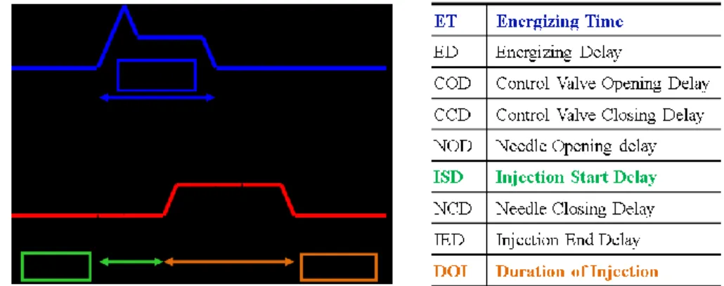
Diesel engines (www.Dieselnet.com). _____________________ 26 Figure 5 – Scheme of Common Rail injector (www.full-repair.com). _ 28 Figure 6 – Modern Diesel combustion strategies plotted in ϕ-T space [29]. ___________________________________________________ 30 Figure 7 – Scheme of in-cylinder stratification with air zone (a) and spray discretization in axial and radial direction. __________________ 40 Figure 8 – Time delays between electric and hydraulic operations in

Common Rail injector systems. __________________________ 42 Figure 9 – Experimental injection flow rate. prail = 1600 bar, ET = 730 μs.

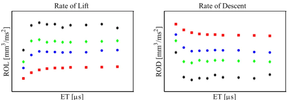
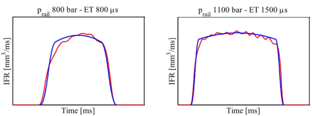
The scales are omitted for confidential issues. _______________ 43 Figure 10 – Injection flow rates experimentally investigated for the model identification. The scales are omitted for confidential issues. ___ 44 Figure 11 – Values of ISD (upper-left), DOI (upper-right), ROL

(lower-left) and ROD (lower-right) experimentally investigated for the model identification. The scales are omitted for confidential issues. ___________________________________________________ 45 Figure 12 – Experimental and predicted Injection Flow Rates for different operating conditions of rail pressure and energizing time. ______ 46 Figure 13 – Typical structure of an impingement spray [74]. ________ 49 Figure 14 – Impingement regimes. ____________________________ 49 Figure 15 – Impingement area [80]. ____________________________ 51 Figure 16 – Mono-dimensional plan for the thermal balance on the fuel

film. ________________________________________________ 53 Figure 17 – Superposition of the in-cylinder pressure in the four

(7)

Index of figures VII

Figure 18 – Engine test bed of the Energy and Propulsion Laboratory at the University of Salerno. Engine A equipment on the left and Engine B equipment on the right side. _____________________ 63 Figure 19 – Intercooler and the dedicated electric fan (left side). Dynamic Fuel Meter AVL 733S (right side).________________________ 64 Figure 20 – Representation of the optical encoder used for the

experimental activity. __________________________________ 65 Figure 21 – In the left picture the thermal mass flowmeter Sensyflow

FMT700-P, in the middle picture the Lambda Meter ETAS LA4 and in the picture on the right the intake manifold equipment. Engine A application. __________________________________ 66 Figure 22 – Turbo speed sensor Micro-Epsilon DZ140 (left side) and

exhaust system equipment (right side). The NOx and pressure

sensors are visible upstream the turbine, the UEGO and another pressure sensor are visible upstream the catalyst. A resistance temperature detector is placed downstream the turbine. _______ 67 Figure 23 – AVL Smoke Meter 415S for Soot analysis (left side) and

AVL pre-filter HSS i60 for Soot filtering before the gas analyzer line (right side). _______________________________________ 68 Figure 24 – Gas analyzer box. On the left side the sampling pump, on the

right side the control module (Advance Optima) and the different gas modules: Uras 14, Multi-FID 14, Magnos 106 and Eco-Physiscs CLD700. ____________________________________________ 69 Figure 25 – The engine control console. From the monitor on the left:

AVL Puma Open for the test bench sensors control; AVL Indicom v2.2 for indicating data treatment and ETAS Inca v7.0 for the management of the ECU. _______________________________ 70 Figure 26 – Communication scheme between user and engine. Actuation

line in blue: input engine variables set by the user; Acquisition line in red: feedback on control strategies from the engine. ________ 72 Figure 27 – Operating conditions investigated for Engine A. The

corresponding EGR percentage is indicated on each operating point. ___________________________________________________ 72

(8)

Figure 28 – Operating conditions investigated for Engine B. EGR = 0. 73 Figure 29 – Operating conditions investigated for Engine C. The

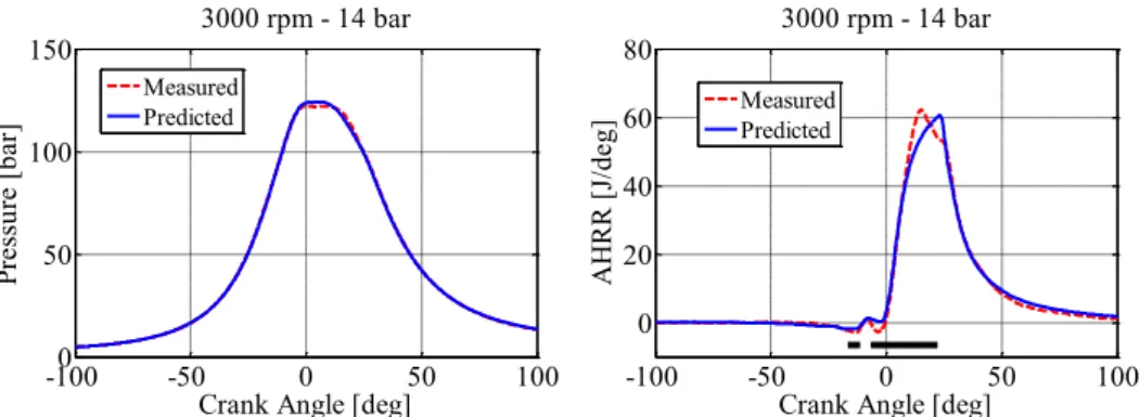
corresponding EGR percentage is indicated on each operating point. ___________________________________________________ 74 Figure 30 – Comparison between measured and predicted in-cylinder

pressure (on the left) and heat release rate (on the right). Engine A, Test Case 1. __________________________________________ 77 Figure 31 – Comparison between measured and predicted in-cylinder

pressure (on the left) and heat release rate (on the right). Engine A, Test Case 2. __________________________________________ 77 Figure 32 – Comparison between measured and predicted in-cylinder

pressure (on the left) and heat release rate (on the right). Engine A, Test Case 3. __________________________________________ 78 Figure 33 – Comparison between measured and predicted Indicated mean

Effective Pressure (IMEP) for the whole set of experimental data. R2 = 0.997. Engine A. __________________________________ 78 Figure 34 – Comparison between measured and predicted engine NOx

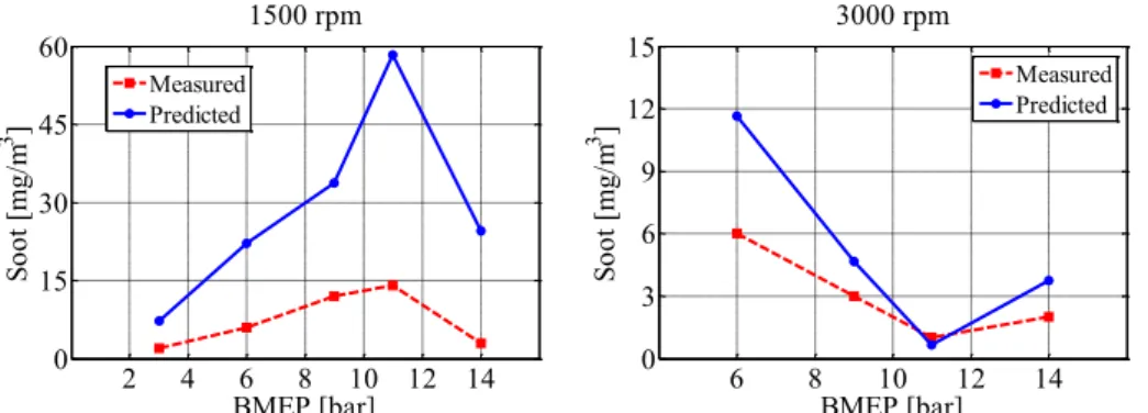
emissions vs. Torque at Engine speed = 1500 rpm (on the left) and at Engine speed = 3000 rpm (on the right). Engine A. _________ 79 Figure 35 – Comparison between measured and predicted engine Soot

emissions vs. Torque at Engine speed = 1500 rpm (on the left) and at Engine speed = 3000 rpm (on the right). Engine A. _________ 80 Figure 36 – Measured in-cylinder pressure (on the left) and apparent heat

release rate (on the right) at different SOImain. Speed 2000 rpm, total

amount of fuel injected 35 mm3, rail pressure 1385 bar. _______ 82 Figure 37 – Experimental values of the normalized specific heat released

vs. injection timing (SOI) for the dataset A. Speed 2000 rpm, total amount of fuel injected 35 mm3, rail pressure 1400 bar. _______ 83 Figure 38 – Experimental values of the normalized specific heat released

vs. rail pressure (prail) for the dataset B. ____________________ 83

Figure 39 – Comparison between measured and simulated in-cylinder pressure (on the left) and apparent heat release rate (on the right). Test Case 1. __________________________________________ 84

(9)

Index of figures IX

Figure 40 – Comparison between measured and simulated in-cylinder pressure (on the left) and apparent heat release rate (on the right). Test Case 5. __________________________________________ 84 Figure 41 – Comparison between experimental and simulated values of

the normalized specific heat released vs. injection timing (SOI) for the data set A. Speed 2000 rpm, total amount of fuel injected 35 mm3, rail pressure 1385 bar. _____________________________ 85 Figure 42 – Index of impingement for the 16 operating conditions

investigated. Simulation results on Engine B. _______________ 87 Figure 43 – Time history of fuel mass impinged on the wall. Five zones

are depicted. Test Case 4 (on the left); Test Case 5 (on the right). 88 Figure 44 – Estimated radius of the impingement area. Test Case 4 (on

the left); Test Case 5 (on the right). _______________________ 88 Figure 45 – Effect of SOI variation on impingement. Reference Test Case nr. 3. Starting SOI = 9.5 °BTDC. _________________________ 89 Figure 46 – Effect of rail pressure on impingement. Reference Test Case

nr. 1. Starting prail = 500 bar. ____________________________ 90

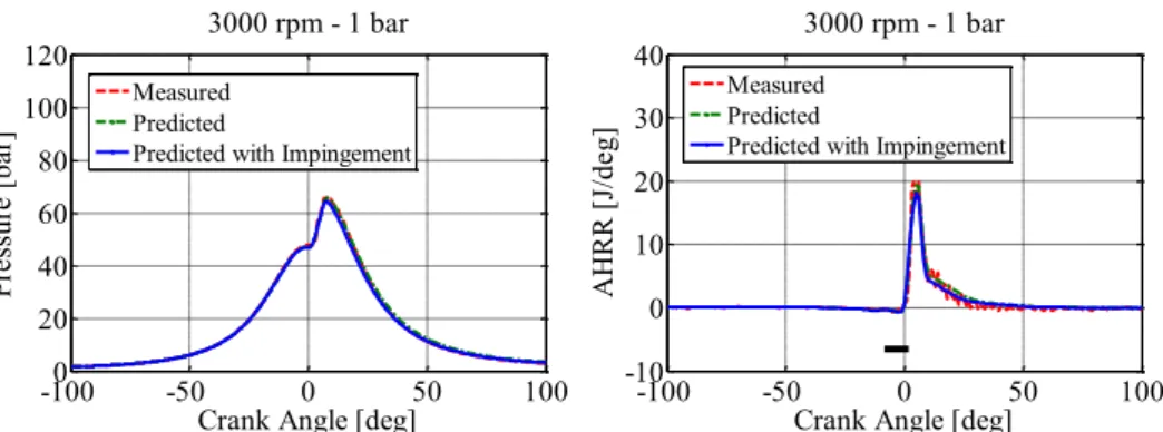
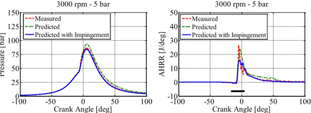
Figure 47 – Comparison between measured and predicted in-cylinder pressure (on the left) and heat release rate (on the right). Engine B, Test Case 2. __________________________________________ 91 Figure 48 – Comparison between measured and predicted in-cylinder

pressure (on the left) and heat release rate (on the right). Engine B, Test Case 4. __________________________________________ 91 Figure 49 – Comparison between measured and predicted in-cylinder

pressure (on the left) and heat release rate (on the right). Engine B, Test Case 5. __________________________________________ 91 Figure 50 – Comparison between measured and predicted in-cylinder

pressure (on the left) and heat release rate (on the right). Engine B, Test Case 6. __________________________________________ 92 Figure 51 – Experimental IMEP vs. evaluated IMEP without accounting

for the impingement model (green circles) and evaluated IMEP by adding the impingement model to the Multi-Zone code (blue

(10)

Figure 52 – Indicated efficiency for the 16 operating condition

investigated. Simulation results on Engine B. _______________ 93 Figure 53 – Comparison between measured and predicted in-cylinder

pressure. Engine C, Test Case 1.__________________________ 94 Figure 54 – Comparison between measured and predicted in-cylinder

pressure. Engine C, Test Case 2.__________________________ 95 Figure 55 – Comparison between measured and predicted in-cylinder

pressure. Engine C, Test Case 3.__________________________ 95 Figure 56 – Comparison between measured and predicted Indicated mean

Effective Pressure (IMEP) for the whole set of experimental data. R2 = 0.995. Engine C. __________________________________ 95 Figure 57 – Comparison between measured and predicted engine NOx

emissions vs. BMEP at Engine speed = 2000 rpm (on the left) and at Engine speed = 2500 rpm (on the right). Engine C. _________ 96 Figure 58 – Comparison between measured and predicted engine Soot

emissions vs. BMEP at Engine speed = 2000 rpm (on the left) and at Engine speed = 2500 rpm (on the right). Engine C. _________ 97 Figure 59 – Simulated in-cylinder pressure (left side) and heat release rate

(right side) at different pilot SOI and fixed EGR and rail pressure. __________________________________________________ 100 Figure 60 – Simulated in-cylinder pressure (left side) and heat release rate

(right side) at different EGR rates and fixed SOI and rail pressure. __________________________________________________ 101 Figure 61 – Simulated in-cylinder pressure (left side) and heat release rate

(right side) at different rail pressure and fixed EGR and SOI. __ 101 Figure 62 – Simulation results: effect of SOI, EGR and prail on IMEP. 102

Figure 63 – Simulation results: effect of SOI, EGR and prail on NOx

emissions. __________________________________________ 103 Figure 64 – Simulation results: effect of SOI, EGR and prail on Soot

emissions. __________________________________________ 103 Figure 65 – Simulation results: effect of SOI, EGR and prail on

(11)

Index of figures XI

Figure 66 – Simulation results: trade-off between combustion noise and IMEP (left side) and trade-off between Soot and NOx emissions

(right side). _________________________________________ 105 Figure 67 – MFB10 (on the left) and MFB50 (on the right) vs SOI at

different variables setting. _____________________________ 108 Figure 68 – Effective power (on the left) and specific fuel consumption

(on the right) vs SOI at different variables setting. __________ 109 Figure 69 – NOx (on the left) and Soot emissions (on the right) vs SOI at

different variables setting. _____________________________ 109 Figure 70 – Combustion noise (on the left) and exhaust temperature (on

the right) vs SOI at different variables setting. ______________ 110 Figure 71 – Trade-off Soot-Combustion noise (on the left) and Soot-NOx

(on the right) at different variables setting. ________________ 111 Figure 72 – Optimization results: base and optimal control variables.

Mass of injected fuel (upper-left), Start of Injection (upper-right), EGR left) and Indicated Mean Effective Pressure (lower-right). _____________________________________________ 114 Figure 73 – Optimization results: performance and emissions in case of

base and optimal control variables. Specific Fuel Consumption (upper-left), Sound Pressure Level (upper-right), NOx (lower-left)

and Soot (lower-right). ________________________________ 114 Figure 74 – Numerical results: emissions and performance (right side) in

case of base and optimal control variables (left side). Test Case 1. __________________________________________________ 118 Figure 75 – Numerical results: emissions and performance (right side) in

case of base and optimal control variables (left side). Test Case 2. __________________________________________________ 118 Figure 76 – Numerical results: emissions and performance (right side) in

case of base and optimal control variables (left side). Test Case 3. __________________________________________________ 119 Figure 77 – Experimental results: emissions and performance (right side)

in case of base and optimal tuning of engine control variables (left side). Test Case 1. ____________________________________ 120

(12)

Figure 78 – Optimization results: percentage difference between base and optimal conditions in case of Multi-Zone analysis and experimental check. Test Case 1. ___________________________________ 121 Figure 79 – Optimization results: from base towards optimal tuning

Model simulation (black-green marker) and experimental test (blue-red marker). Optimization constrains: Model confidence area in yellow, Experimental confidence area in orange. Test Case 1. _ 122 Figure 80 – Optimization results: Comparison between simulated and

measured in-cylinder pressure left), heat release rate (upper-right) and injection flow rate (lower). Test Case 1. __________ 123 Figure 81 – Experimental results: emissions and performance (right side)

in case of base and optimal tuning of engine control variables (left side). Test Case 2. ____________________________________ 124 Figure 82 – Optimization results: percentage difference between base and optimal conditions in case of Multi-Zone analysis and experimental check. Test Case 2. ___________________________________ 124 Figure 83 – Optimization results: from base towards optimal tuning

Model simulation (black-green marker) and experimental test (blue-red marker). Optimization constrains: Model confidence area in yellow, Experimental confidence area in orange. Test Case 2. _ 125 Figure 84 – Optimization results: Comparison between simulated and

measured in-cylinder pressure left), heat release rate (upper-right) and injection flow rate (lower). Test Case 2. __________ 126 Figure 85 – Experimental results: emissions and performance (right side)

in case of base and optimal tuning of engine control variables (left side). Test Case 3. ____________________________________ 127 Figure 86 – Optimization results: percentage difference between base and optimal conditions in case of Multi-Zone analysis and experimental check. Test Case 3. ___________________________________ 127 Figure 87 – Optimization results: from base towards optimal tuning

Model simulation (black-green marker) and experimental test (blue-red marker). Optimization constrains: Model confidence area in yellow, Experimental confidence area in orange. Test Case 3. _ 128

(13)

Index of figures XIII

Figure 88 – Optimization results: Comparison between simulated and measured in-cylinder pressure left), heat release rate (upper-right) and injection flow rate (lower).Test Case 3. ___________ 129 Figure 89 – Comparison between measured and predicted engine control

variables: Air mass left), Manifold Temperature (upper-right), pressure of residual gases (lower-left), temperature of

residual gases (lower-right). ____________________________ 135 Figure 90 – Comparison between measured and simulated in-cylinder

pressure, with and without the regression models (on the left) and apparent heat release rate (on the right). Test Case 2. ________ 136 Figure 91 – Comparison between measured and simulated in-cylinder

pressure, with and without the regression models (on the left) and apparent heat release rate (on the right). Test Case 3. ________ 136 Figure 92 – Comparison between measured and simulated IMEP, with

and without the regression models, at 1500 rpm (on the left) and at 3000 rpm (on the right). _______________________________ 136 Figure 93 – Comparison between measured and simulated SPL, with and

without the regression models, at 1500 rpm (on the left) and at 3000 rpm (on the right). ____________________________________ 137 Figure 94 – Comparison between measured and simulated NOx, with and

without the regression models, at 1500 rpm (on the left) and at 3000 rpm (on the right). ____________________________________ 137 Figure 95 – Comparison between measured and simulated Soot, with and

without the regression models, at 1500 rpm (on the left) and at 3000 rpm (on the right). ____________________________________ 137

(14)

Index of tables

Table 1 – Values of rail pressure (prail) and energizing time (ET)

experimentally investigated for the injection rate identification. _ 44 Table 2 – Engines Data _____________________________________ 62 Table 3 – Sensors accuracy __________________________________ 64 Table 4 – Injection parameters. _______________________________ 75 Table 5 – Entrainment/Ignition parameters. ______________________ 76 Table 6 – Test cases considered for model validation. Engine A. _____ 77 Table 7 – Set-points of the main control variables for dataset A. prail =

1385 bar, pboost = 1.5 bar. _______________________________ 81

Table 8 – Set-points of the main control variables for dataset B. pboost =

1.5 bar, EGR = 17.9÷22.3%. _____________________________ 81 Table 9 – Test cases considered for model validation. Engine B. _____ 86 Table 10 – Test cases considered for model validation. Engine C. ____ 94 Table 11 – Set-points of the combustion control variables investigated to

analyze the impact on performance and emissions. ___________ 99 Table 12 – Operating conditions investigated for the trade-off analysis.

__________________________________________________ 104 Table 13 – Rail pressure [bar] as function of total amount of fuel injected

(Qinj) and speed for basic calibration. Provided by Magneti Marelli

Powertrain. _________________________________________ 106 Table 14 – Potential Power Saving [W] as function of total amount of fuel

injected (Qinj) and speed in case of SDA application (maximum rail

pressure achievable 800 bar). Provided by Magneti Marelli

Powertrain. _________________________________________ 106 Table 15 – Variables setting in case of basic configuration and tuning

procedure. Speed = 4000 rpm, full load, torque = 160 Nm, EGR = 0. Engine C. ________________________________________ 107 Table 16 – Operating conditions selected as test cases for the optimization

analysis. Engine C. ___________________________________ 112 Table 17 – Operating conditions selected as test cases for the optimization

(15)

Nomenclature

AFR AHRR ATDC BDC BMEP BSFC CAD CAI CFD CI CLD CN COD CRF DI DOC DOI DPF DT ECE ECU ED EGR air-fuel ratio

apparent heat release rate after top dead centre bottom dead centre

brake mean effective pressure brake specific fuel consumption crank angle degree

gasoline controlled auto-ignition computational fluid dynamics compression ignition

chemi-luminescence detector combustion noise

control valve opening delay FIAT research centre direct injection

Diesel oxidation catalyst duration of injection Diesel particulate filter dwell time

urban driving cycle electronic control unit energizing delay

(16)

EMS ET EUDC FFT FID FSN GHG HCCI I/O IDI IFR IMEP ISD ISFC IVC JTD LNT LTC MDA MFB MK NDIR NOD NSHR PCCI

engine management systems energizing time

extra urban driving cycle fast fourier transform flame-ionization detector filter smoke number greenhouse gas

homogeneous charge compression ignition input/output

indirect Diesel injection injection flow rate

indicated mean effective pressure injection start delay

indicated specific fuel consumption intake valve closing

UniJet Turbo-Diesel (FIAT abbreviation) lean NOx trap

low temperature combustion measure data analyser mass fraction burned modulated kinetics

nondispersive infrared sensor needle opening delay

normalised specific heat released pre-mixed charge compression ignition

(17)

Nomenclature XVII PCI prail Qmax Qinj R2 RCCI Re ROD ROL Sc SCR SDA SDE Sh SHR SI SOC SOI SPL TDC UEGO VGT VVA We

premixed compression ignition rail pressure

static fuel flow rate amount of fuel injected correlation index

reactivity controlled compression ignition Reynolds number

rate of descent rate of lift Shmidt number

selective catalytic reduction solenoid direct actuation small Diesel engine Sherwood number specific heat released spark ignition

start of combustion start of injection sound pressure level top dead centre

universal exhaust gas oxygen (sensor) variable geometry turbine

variable valve actuation Weber number

(18)

CHAPTER 1 Introduction

The interest in Diesel engines for automotive application has dramatically grown in the last decade, due to the benefits gained with the introduction of Common Rail system and electronic control. A strong increase in fuel economy and a remarkable reduction of emissions and combustion noise have been achieved, thanks to both optimized fuelling strategy and advanced fuel injection technology. Namely, the improvement of injector time response, injection pressure and nozzle characteristics have made feasible the operation of multiple injections and have enhanced the fuel atomization. The actuation of early pilot and pre injections enhances the occurrence of a smoother combustion process with benefits on noise. Improved fuel atomization enhances the air entrainment making the combustion cleaner and more efficient, thus reducing both particulate emissions and fuel consumption but with a negative impact on NOx emissions [1][2][3][4][5][6][7][8][9].

On the other hand the recourse to Exhaust Gas Recirculation (EGR) lowers in-cylinder peak temperature and NOx emissions but with a

negative impact on particulate emissions. In the last years many efforts are addressed towards new combustion concepts, in order to face with the Soot/NOx trade off and the increasingly restrictive emission standards.

Earlier injections and large EGR rate promote premixed combustion and lead to lower peak temperature, with benefits on both particulate and NOx

emissions. The drawback is the increase of combustion noise, due to the large delay of premixed combustion up to the Top Dead Centre (TDC) that results in a dramatic and sharp increase of in-cylinder pressure [9].

In this context, it is clear that a suitable design of engine control strategies is fundamental in order to overcome with the simultaneous and opposite impact of combustion law on NOx/Soot emissions and

combustion noise. Nevertheless the large number of control variables (i.e. injection pattern, EGR, VGT) makes the experimental testing extremely expensive in terms of time and money. Massive use of advanced mathematical models to simulate engine and system components

(19)

Introduction 19

(mechanical and electronic devices) is therefore recommended to speed up the design and optimization of engine control strategies.

1.1 Technology evolution in Diesel engines

Compression ignition engine (CI) evolution has been affected by the spark ignition engine (SI) on automotive market. With regard to the thermodynamic cycles of both engines, it comes out that at the same operating conditions (injected fuel and speed) and with the same dimensions for piston and cylinder (equal compression ratio), the SI engine reveals higher efficiency. In Figure 1 are reported the two ideal thermal cycles.

Figure 1 – Scheme of ideal thermal cycle for both otto (left side) and Diesel (right side) engine

Referring to isentropic compression/expansion phases (1-2 and 3-4) and adiabatic combustion/exhaust phases (2-3 and 4-1), the thermal efficiency evaluation will be simplified:

(20)

















4 1 , 3 2 4 1 , 3 2 1 1 1 1 1 1 1 1 1 1 1 1

out in out out th in in in v th otto v v v c th diesel p v c W Q Q Q Q Q Q mc T T mc T T r mc T T r mc T T r r                            _{ } _   _  _ ( 1 )

where Wout is the net work transferred to the piston, Qin is the thermal

energy provided by the fuel combustion, Qout is the thermal energy that

flows out the engine during the exhaust phase, m is the mass of the working fluid, cv and cp are the specific heats at constant volume and

pressure respectively, γ is the specific heat ratio, Ti are temperatures, rv is

the volumetric compression ratio (ratio between the maximum and the minimum cylinder volume) and rc is the cut-off ratio (ratio of the cylinder

volume at the beginning and end of the combustion process in Diesel engines)1.

Of course the actual thermal efficiency will be significantly lower due to heat and friction losses. Nevertheless, comparing the two formulas, it can be seen that for a given compression ratio, the ideal Otto cycle will be more efficient since rc is always higher than 1 as well as the term

1 1 1 c c r r       _ 

 . Despite this, gasoline limits the maximum pressure in the combustion chamber in order to avoid knocking phenomena, therefore SI engines can’t get compression ratios higher than 11-12, as reported in Figure 2. On the other hand, in a CI engine the self-ignition is the desired behaviour, so compression ratios are allowed up to 20-22 and the efficiency becomes comparable to the SI engines.

1 1 2 3 2 displaced clearance v clearance c V V V r V V V r V    

(21)

Introduction 21

Figure 2 – Thermal efficiency trend vs. compression ratio in ideal conditions.

Another important difference between SI and CI engines concerns the combustion process. In SI engines the air-fuel mixture ignition starts after the spark of a glow plug, located in the combustion chamber. The flame front spreads out from the glow plug up to the whole combustion chamber without strong pressure gradients if the detonation is avoided. In CI engines instead, part of the total fuel amount is injected before the Top Dead Centre (TDC). When pressure and temperature reach the conditions of auto-ignition, all the fuel injected burn instantaneously, provoking a strong in-cylinder pressure increase. This phase is called ‘premixed

combustion’ and it is followed by a diffusive combustion phase, where

high in-cylinder temperatures bring about a gradual evaporation and combustion of the following injected fuel [10][11].

High pressure gradients during the premixed combustion phase cause strong and cyclic mechanical stresses. Therefore, aspirated Diesel engines are more massive compared to the Gasoline engines with the same power, from the structural point of view. Furthermore, stresses cause vibration and consequently unwelcome noise, typical of old Diesel engines [12][13]. These aspects limited for a long time the use of Diesel engines for industrial systems aimed at the production of electric energy, naval propulsion systems and heavy means for land traction. Up to now, Diesel engine got a remarkable evolution. The technology evolution carried out side by side with new applications and new suitable market sectors, depending on the economical context, on the social period and the different places. Anyway, strictly dependent on the evolution of SI engines.

For many years the Diesel engine evolution mainly interested the Compression ratio [/] T he rm al E ff ic ie nc y [/ ]

Ideal gas condition (  = 1.4 )

SI range CI range 0 5 10 15 20 25 0 0.2 0.4 0.6 0.8 1 SI, CI (rc=1) CI (rc=2) CI (rc=3) CI (rc=4)

(22)

technology of the fuel path system. In 1908 fuel oil was injected in the cylinder by means compressed air for the first time. The pneumatic fuel system made the Diesel engine strongly competitive compared to the steam engine, his antagonist in that time. Higher powers could be reached with the same engine weight and the big carbon containers could be avoided, therefore Diesel engine became leader in sea applications [14].

In the early 20’s the first mechanical injection pump was designed and its mass production started. Precision and fast operations allowed this system to be applied on industrial vehicles. For the first time, the fuel was injected directly in the cylinder by means of an atomizer or injector, which function was to turn the fuel into small drops in order to aid its evaporation process and to lower the ignition delay [14][15].

Nevertheless, the development of direct injection engines (DI) with small piston displacement for automotive applications was not possible. Injector holes manufacturing was very complicated since very small dimensions were needed for the typical fuel flows used in small displacement engines, furthermore they were still very noisy. With the aim to overcome these difficulties the indirect injection or pre-chamber engine (IDI) was born [14].

In IDI engines fuel is not injected directly in the cylinder, but in a smaller pre-chamber that is arranged into the cylinder head. The arrangement comprises a body part forming the first end of the chamber and a separate nozzle part for discharging fluids from the pre-chamber into the main combustion pre-chamber of the cylinder. With this configuration combustion starts in the pre-chamber and follows in the cylinder thanks to the gas expansion. The aim was to avoid an instantaneous ignition of the whole mixture and consequently high pressure peaks that make the engine very noisy and transmit strong vibrations to the chassis [10][13].

In the late 70’s the technology evolution allowed the introduction of the direct injection in Diesel engines, guaranteeing a remarkable reduction in fuel consumption. This evolution step, both with the development of the first boosting system for automotive applications in the same years, represented the most significant improvements in CI engines technology, making it really competitive with the SI engines.

(23)

Introduction 23

1.2 The Common Rail injection system

In the last two decades, the Common Rail injection system has been introduced in passenger car and truck Diesel engines. This injection system offers more degrees of freedom for combustion optimisation and has significant advantages compared with cam driven fuel injection systems. In a Common Rail injection system the fuel is pressurised by a hydrostatic high-pressure pump and fed to a ‘Common Rail’ arranged near the injectors for all cylinders. The injection event is electronically controlled by a solenoid valve. The rail pressure is controlled by a pressure control valve.

The key advantage of the Common Rail system is that the pressure generation and the injection process are separated and, over the whole engine operating range, the start and end of injection as well as the pressure within permissible/useful limits can be chosen independently of the engine speed and load. The average rail pressure remains constant prior to the injection and the injected quantity is the result of the rail pressure, the flow losses in the injector and the opening duration of the electromagnetic valve.

The injected quantity can be varied by the injector needle lift control. By opening and closing the solenoid valve, the pressure in the control volume is modulated and, thereby, the needle opens and closes. The solenoid valve has switching times which are smaller than 200 ms and this is essential for small quantities (1-2 mm3 per injection) for example for pilot injection. The rate of injection, i.e. the rate at which fuel is injected as function of crank angle (dQ/dθ) is an important feature of the injection process which affects the combustion process, fuel consumption and emissions.

1.2.1. Historical steps evolution

In principle, the Common Rail system has been known since many years. James McKechnie was the General Manager of the Shipyard and Armaments Factory of Vickers Sons and Maxim Ltd. in Barrow-in-Furness (UK); in 1910 he was elected to the Board of Vickers Ltd and he received in the same year patent 27 579. In Figure 3 is represented the scheme of the first patented Common Rail injection system, where F is

(24)

the mechanically operated valve, f1 is the lever, f2 is the cam, f3 is the shaft, C the fuel actuating plunger and a1 the nozzle holes.

Figure 3 – First patented Common Rail injection system [16].

Due to his position in the company, McKechnie was not likely to have been the real inventor, although he was named as inventor of several Vickers patents related to fuel injection:

• NO. 27 579, 1910, ‘solid injection’ with accumulator between pump and mechanically operated injector

• NO. 26 227, 1911, oval tube accumulator

• NO. 24 127 (with accumulator), NO. 24 153 (without accumulator), both in 1912 for constant pressure pump

• NO. 1 059, 1914, patent related to injector nozzle design, in particular the important ratio of nozzle hole diameter to hole length. Also the hydraulically actuated needle is mentioned, but Vickers always used mechanical needle actuation.

All Vickers-designed Diesel engines had Common Rail injection up to 1943 when they built their last engine.

An early Common Rail system was developed at Atlas-Imperial after World War I. It had a high-pressure pump with multiple plungers which delivered fuel to an accumulator, a pressure relief valve and to mechanically operated nozzles. The spring-loaded nozzle valves were lifted mechanically by push rods and levers actuated by cams [15][17].

A Common Rail system using for the first time an electromagnetically actuated injector was produced by Atlas Imperial Diesel Engine of Oakland, California in the early 1930s and the injection pressures were between 280 and 560 bars [15][18]. The Atlasco system was designed for ‘small, high-speed Diesel engines’ and had fuel supplied to the valve at

(25)

Introduction 25

constant pressure from an accumulator; metering was carried out by variation of the opening period.

In the 1960s the French company Société des Procédés Modernes d’Injection (SOPROMI) developed an electromechanically actuated injection system. Also, in France, the Société Française d’études et de development de l’injection (Sofredi) had patented, in 1970, an electromagnetically controlled fuel injector [19]. Subsequent designs were similar.

During the 1960s and 1970s development concentrated on accommodating the high-pressure fuel storage (accumulator volume) within the injector. In the middle of the 1980s, the ‘Common Rail’ with short pipes to the injectors was introduced. A high-pressure variable delivery radial piston pump was designed and tested and reached up to 2000 bar pressure [20][21]. Apart from tests on the small high-speed engine, the Common Rail system was investigated on truck Diesel engines. By 1988 a prototype Iveco TurboDaily was equipped with a Common Rail system for road tests.

In 1986 Fiat presented the Croma 1.9, the first passenger car with a turbocharged Diesel engine with direct injection. Fiat became more and more interested in the Common Rail injection system and decided to initiate a strategic project in order to verify the industrial feasibility of the Common Rail injection system. In 1989, a consortium named Élasis established a research centre at Bari specialising in fuel injection equipment; Magneti Marelli joined the consortium.

In the following years in a close inter-functional co-operation Élasis and Fiat Research Centre (Centro Ricerche Fiat, CRF) succeeded in overcoming the key technological problems and improved the design mainly from a manufacturing point of view. As examples, the two-needle system was introduced and the seat of the control needle was changed to a spherical seat. CRF conducted rig and engine tests with the system now called UniJet, and introduced measures to reduce shot-to-shot and injector-to-injector variations [14]. This was followed by vehicle tests and demonstrated the advantages of the Common Rail system in cars [22].

By the end of 1991 the second generation UniJet system prototypes were fully demonstrating their functional potential. At the end of 1992 the preliminary reliability and consistency both on engines and in vehicles was satisfactorily passed. By the end of 1993 a pre-industrialised version of the UniJet system was available.

(26)

In spring 1994 the Fiat Group signed an agreement with Robert Bosch for the industrialisation and further development of the system. In October 1997 Fiat introduced into the passenger car market the Alfa Romeo 156 JTD model, equipped with two DI Diesel engines (4 cylinder 1.9 dm3 and 5 cylinder 2.4 dm3) both using the UniJet system produced by Robert Bosch [14][20]. CRF is continuing its efforts to improve Common Rail systems by the MultiJet-system, which permits injection of a certain fuel quantity in up to five injections (multiple injection).

Although today’s Common Rail system has several important advantages compared with conventionally used fuel injection systems, it has still considerable scope for improvement. Also systems with piezoelectric actuation have been developed and are in production (Siemens Automotive). They utilise the piezoelectric effect in that across non-conductive crystals an electric field or potential difference is applied which produces a mechanical deformation. Piezoelectric actuation of the control valve is faster than with solenoids [14][23].

1.2.2. Systems components and main features

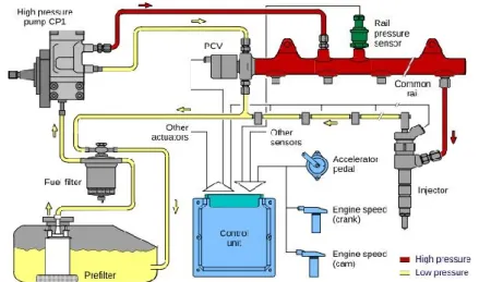
The main elements of a Common Rail Diesel injection system are a low pressure circuit, including the fuel tank and a low pressure pump, a high pressure pump with a delivery valve, a Common Rail and the electro-injectors (Figure 4) [24][25][26][27]. Few details illustrate the injection operation.

Figure 4 – A block scheme of the Common Rail injection system for Diesel engines (www.Dieselnet.com).

(27)

Introduction 27

The low pressure pump sends the fuel coming from the tank to the high-pressure pump. Hence the pump pressure raises, and when it exceeds a given threshold, the delivery valve opens, allowing the fuel to reach the Common Rail, which supplies the electro-injectors. The Common Rail hosts an electro-hydraulic valve driven by the Electronic Control Unit (ECU), which drains the amount of fuel necessary to set the fuel pressure to a reference value. The valve driving signal is a square current with a variable duty cycle (i.e. the ratio between the length of ‘on’ and the ‘off’ phases), which in fact makes the valve to be partially opened and regulates the rail pressure.

The high pressure pump is of reciprocating type with a radial piston driven by the eccentric profile of a camshaft. It is connected by a small orifice to the low pressure circuit and by a delivery valve with a conical seat to the high pressure circuit. When the piston of the pump is at the lower dead centre, the intake orifice is open, and allows the fuel to fill the cylinder, while the downstream delivery valve is closed by the forces acting on it. Then, the closure of the intake orifice, due to the camshaft rotation, leads to the compression of the fuel inside the pump chamber. When the resultant of valve and pump pressures overcomes a threshold fixed by the spring preload and its stiffness, the shutter of the delivery valve opens and the fuel flows from the pump to the delivery valve and then to the Common Rail.

As the flow sustained by the high pressure pump is discontinuous, a pressure drop occurs in the rail due to injections when no intake flow is sustained, while the pressure rises when the delivery valve is open and injectors closed. Thus, to reduce the rail pressure oscillations, the regulator acts only during a specific camshaft angular interval (activation window in the following), and its action is synchronized with the pump motion.

The electro-injector is the heart of the Common Rail multiple injection system and its scheme is shown in Figure 5. The main elements of an electro-injector for Diesel engines are a control chamber and a distributor. The former is connected to the rail and to a low pressure volume, where both inlet and outlet sections are regulated by an electro-hydraulic valve. During normal operations the valve electro-magnetic circuit is off and the control chamber is fed by the high pressure fuel coming from the Common Rail. When the electro-magnet circuit is excited, the control chamber intake orifice closes while the outtake orifice opens and so a

(28)

pressure drop occurs. When the injection orifices open, the cylinders receive the fuel. The Energizing Time depends on the fuel amount to be injected and it is the only measurable variable for automotive application.

Figure 5 – Scheme of Common Rail injector (www.full-repair.com).

The injector shown in Figure 5 is a solenoid-operated injector. Traditional Diesel injectors use electromagnetic, or solenoid, controls. The electronic engine management system sends an electrical signal to activate the mechanical valve that controls fuel flow through the injector. The technology is well-known, reliable, cost-effective, and the unit is physically smaller than piezo units. But solenoid injectors tend to vibrate more than piezo units, creating more noise.

In a piezo injector, the electronic engine management system also sends an electrical signal to the valve. But the unique property of a piezo crystal is that it changes shape when exposed to electric current. The actual movement is microscopic, but enough to make the piezo element act as the valve. Piezo injectors are quieter and more precise than solenoid units, a benefit in a microsecond environment, but they are more expensive.

(29)

Introduction 29

In both cases, the Common Rail principle remains the core of Diesel injection systems. A single (common) high-pressure fuel line is connected to individual injectors at each cylinder.

In the described system, the pressure regulation aims at supplying the engine precisely with the specific amount of fluid and the proper air/fuel mixture demanded by its speed and load. Of course, this requires a good mathematical model necessary to develop both an appropriate control strategy and an effective controller tuning. However, the strong nonlinearities due to complex fluid-dynamic phenomena make the design of dynamic models very hard. In fact, even very complex fluid-dynamic models may not be able to describe the system behaviour in every working condition [27][28]. On the other hand, it is possible to manage a large number of engine control variables, therefore different strategies can be defined as an alternative to the technical evolution for both improving the engine performance and for reducing pollutant emissions.

1.3 Innovative combustion concepts in Diesel engines

In the last years many efforts are addressed towards new combustion concepts, in order to face with the Soot/NOx trade off and the increasingly

restrictive emission standards. Revolutionary in-cylinder combustion strategies and exhaust emission after-treatment systems have been developed for this aim. Emission after-treatment devices, however, have problems in terms of their cost and durability. Since emission after-treatment systems such as Diesel Particulate Filters (DPF), Lean NOx

Trap (LNT) and Selective Catalytic Reduction (SCR) systems also often increase fuel consumption, in-cylinder technologies for emission reduction have therefore been the focus of intense research [29]. Accordingly, reduction of NOx and Soot in-cylinder has been investigated

by many researchers. Most of the current strategies can be placed in the category of premixed Low Temperature Combustion (LTC).

LTC includes a variety of innovative and different premixed combustion mechanism discovered by many researchers, such as

premixed charge compression ignition (PCCI) [30][31][32],

(30)

premixed compression ignition (PCI), modulated kinetics (MK), reactivity controlled compression ignition (RCCI) [29] etc.

Figure 6 – Modern Diesel combustion strategies plotted in ϕ-T space [29].

A common feature of LTC is to enhance the premixing of fuel and air and to keep combustion temperature low in order to simultaneously avoid NOx and Soot formations [38][39][40]. LTC can also potentially offer low

fuel consumption due to short combustion duration. High thermal efficiency and low emissions of NOx, Soot, HC and CO require a precise

control of LTC process on auto-ignition and combustion timing in order to make the cylinder charge of reacting mixture combust in the region of concurrent low emissions on the ϕ-T diagram commonly used in combustion analysis (Figure 6). LTC usually uses a high EGR rate, high boost pressure, high compression ratio, lean mixture and fast burn rate to achieve extremely low engine-out NOx and Soot emissions, accordingly

with the standards, simply by means of in-cylinder solutions. EGR and intake valve closing (IVC) timing are usually used in PCCI or HCCI to control optimal Diesel combustion phasing.

Early PCCI refers to injecting fuel far before TDC, and the ignition and burning events occur generally before TDC. Late PCCI refers to injecting fuel after TDC, and the ignition and burning events occur far after TDC. Both early and late PCCI can rely on long ignition delays to achieve good mixing and produce very low NOx and Soot at low break

mean effective pressure (BMEP). Early PCCI has good stability and low fuel consumption, but it requires a higher EGR rate, and generates higher peak cylinder pressure, higher combustion noise, and a more limited BMEP range than late PCCI. Late PCCI has a narrower combustion

(31)

Introduction 31

stability range and hence usually needs a combustion sensor to control it. Stanton ([41]) shows that early PCCI is superior to late PCCI and smokeless rich combustion at low speeds and loads in terms of thermal efficiency at the same low NOx level.

LTC usually encounters problems of high HC and CO emissions due to complications in ignition control, and sometimes the problems are severe enough to lead to high brake specific fuel consumption (BSFC). The high HC and CO emissions are due to relatively low volatility of Diesel fuels, fuel condensation and flame quenching on the combustion chamber surface or in the crevice, and spray-wall impingement [42]. Liquid fuel impingement on walls sometimes can also make LTC challenging in Soot control.

Although HC and CO can be controlled by using a Diesel oxidation catalyst (DOC), high BSFC and high CO2 emission are still challenges for

LTC to meet greenhouse gas (GHG) regulations. The fuel efficiency benefit of Diesel HCCI/PCCI is limited by the current inability of adequately controlling optimal combustion phasing and liquid fuel impingement, especially at high loads. In kinetically controlled LTC, there is only a small combustion window for simultaneous low emissions and high thermal efficiency, and this window is very difficult to control at various speeds and loads. The difference of BSFC between LTC and conventional Diesel combustion resides from a complex combination of several aspects as follow. Controlled combustion timing, leaner and premixed mixture, less in-cylinder heat transfer losses, less intake oxygen of LTC may offer some combined advantages in thermal efficiency (e.g., total 7%). However, lower compression ratio, reduced combustion efficiency (related to excessive HC and CO emissions), and hotter intake charge temperature may offset the gain in thermal efficiency to a certain extent (e.g., 3%). Finally, there may be either a net gain or loss in BSFC for LTC, compared with conventional combustion [40].

The low-end bound of load range in LTC operation is limited by ignition and combustion stability. Running LTC at high loads is also an unresolved challenge. The high-load operation of LTC is limited or prohibited by high equivalence ratio (low air-fuel ratio), high Soot emission, and excessively high peak cylinder pressure and rise rate. The load span from the minimum to the maximum achievable in PCCI/HCCI is affected by the fuel cetane number. The challenge of implementing LTC not only comes from controlling stable combustion phasing (via

(32)

EGR and VVA) and controlling the transitions between different combustion modes from low loads to high loads (and vice versa), but also comes from the fact that the combustion chamber and injector nozzle configuration must be compatible with conventional combustion. Although the speed-load range of LTC has been extended through advanced combustion development, currently conventional Diesel combustion still has to be used at high loads. It should be noted that high-load or full-high-load conditions often are critical modes used in Diesel engine system design.

In kinetics-controlled PCCI, seeking an optimum fuel blend to control reactivity is an effective way of extending the BMEP range of HCCI/PCCI. It is worth noting a new emerging combustion mode, RCCI. It is a combustion mode between Diesel HCCI and gasoline controlled auto-ignition (CAI) in terms of combustion chemistry. The concept of RCCI is to achieve high thermal efficiency and low NOx and Soot

emissions across a wide range of engine loads by the mixing of fuels of varied reactivity in the cylinder. RCCI uses direct injection of Diesel fuel plus port injection of gasoline or direct added injection of gasoline (e.g., 75-90% gasoline plus 25-10% Diesel) to control in-cylinder charge conditions and operate in a compression-ignition cycle. It is well known that the high volatility of fuel (e.g., Diesel and gasoline mixture in-cylinder) can help mixing. As Reitz pointed out [29], Diesel fuel ignites easily but is difficult to vaporize, while gasoline is difficult to ignite but can vaporize easily. Both fuels have benefits and drawback in terms of controlling HCCI/PCCI. Diesel is good for low-load premixed combustion, but can cause combustion to occur too early at high loads, and therefore Diesel fuel encounters a load limit at high BMEP. On the contrary, gasoline gives poor combustion at low loads but can offer good combustion at high loads. Therefore, dual-fuel compression ignition combustion may offer a viable path to resolve the load range limitation problem of HCCI/PCCI in order to properly control combustion timing and cylinder pressure rise rate, and extend the loads limits of either pure Diesel or gasoline.

It should be noted that adding a Diesel-to-gasoline ratio into LTC control provides another powerful dimension of combustion control parameters. RCCI has much higher HC and CO emissions (just like gasoline engines) than conventional Diesel combustion and therefore requires HC and CO oxidation catalysts. Although the combustion

(33)

Introduction 33

efficiency of RCCI is lower than conventional Diesel combustion (e.g., 97% vs. 99% due to excessive HC emissions), the benefits of RCCI in terms of combustion timing, leaner mixture’s equivalence ratio, much reduced EGR rate and reduced pumping/heat losses, and less in-cylinder heat transfer can offer a net gain of several percentage points of thermal efficiency increase. It was reported that RCCI can offer approximately 20% improvement in thermal efficiency over conventional Diesel combustion while meeting NOx and Soot emissions without

after-treatment; thermal efficiencies greater than 50% for both heavy-duty and light-duty engines can be reached [29].

1.4 State of art of combustion and fuel injection

modelling in Diesel engines

In this context, it is clear that a suitable design of engine control strategies is fundamental in order to overcome with the simultaneous and opposite impact of combustion law on NOx/Soot emissions and

combustion noise. Nevertheless the large number of control variables (i.e. injection pattern, EGR, VGT) makes the experimental testing extremely expensive in terms of time and money. Massive use of advanced mathematical models to simulate engine and system components (mechanical and electronic devices) is therefore recommended to speed up the design and optimization of engine control strategies.

Numerical models aimed at Diesel engines simulation can be classified into three categories: zero-dimensional models, quasi-dimensional models and multi-quasi-dimensional models [7][43][44][45]. Zero-dimensional models or single-zone models assume that the in-cylinder gas mixture has the same temperature and chemical composition at each time step. Many works in literature ([3][46][47][48][49]) refer to this kind of models to predict with good accuracy and low computational burden the engine performance. Nevertheless, these models are not able to calculate in-cylinder temperature and gas properties variations, which are fundamental to predict the pollutant emissions. Multi-dimensional models instead, solve partial differential equations aimed at describing the in-cylinder fluids flow with high precision, by means close spatial grids. In

(34)

spite of this, some processes are still simulated by means phenomenological sub-models and results are strongly affected by the calibration parameters. As a consequence, it is not possible guarantee high accuracy levels for each operating condition. Furthermore, long calculation times and the necessary data storage make these models just useful for design applications (e.g. combustion chamber), but not properly for planning engine control strategies.

Quasi-dimensional models are the middle way between multi-dimensional and zero-multi-dimensional models, since they match advantages of both types. Quasi-dimensional models solve mass and energy equations without taking into account the integration of momentum. These latter are able to provide information about the spatial distribution of temperatures and gas composition inside the cylinder, not in detail such as multi-dimensional models but with a computational effort considerably lower.

Up to now a large number of quasi-dimensional models have been developed, in literature can be found models with only two zones ([8][49]) and models with more than one hundred ([5][6][50][51]). These models differ not only because of the whole number of zones, but especially because of complexity and accuracy of their sub-models aimed at the description of penetration, atomization, evaporation, mixing and combustion. Some Multi-Zone models simulate mixing and combustion without accounting for the spray dynamic ([52][53]). For example Kamimoto et al. ([52]) assumed an instantaneous fuel vaporization just after the injection. Others, such as the model proposed by Lipkea and DeJoode ([53]), considered atomization and evaporation processes so fast compared to the mixing that was worth to neglect them: the spray is modelled as a vapour jet and the liquid phase was not considered. Actually, atomization and evaporation process could be neglected only in case of in-cylinder conditions close to the fuel critical point. Therefore, these kind of models cannot be applied on a wide engine working range. One of the most evolved Multi-Zone was developed by Hiroyasu et al. in 1983 ([5]) and afterwards adopted and improved by Jung and Assanis ([6]). The spray was divided into a large number of zones both along longitudinal and radial direction and their time evolution is simulated. Cone angle, penetration, mean Sauter diameter and break-up length are modelled by means experimental relations that came out from studies in environment at constant pressure. Furthermore, swirl and fuel wall

(35)

Introduction 35

impingement effects were taken into account with proper empirical coefficients. It is worth noting that, for last generation of Diesel engines, both injection pressure and in-cylinder pressure during the injection, as well as the temperature at the same instant, are considerably higher than those considered by Hiroyasu et al. ([5][54]). Although many Multi-Zone models have been cited, it is still not easy to simulate fairly both premixed and diffusion combustion phase. For example, Kong et al. ([82]) assumed combustion velocity as function of the total amount of air entrained during the premixed combustion, without accounting for the mixing. Many other works instead ([5][55]) consider air-fuel mixture combustion in stoichiometric condition. These models overestimate in-cylinder temperature and hence NOx emission. As well, they are

extremely sensitive to the entrained air and coefficients, completely different among the literature, are used to calibrate the entrainment and to validate the model [6]. Finally, in other works ([56]), the combustion sub-model is based on a simplified turbulent approach, with the aim to account for the effect of mixing on combustion. Many Multi-Zone models do not account for the radiative heat exchange ([5][55]), whose contribution on the whole thermal exchange can be very significant (from 5% up to 50%) [10].

In all the mentioned models, one of the important inputs are the injected mass and/or the shape of the injection event. Many Common Rail injector models are reported in the literature [57][58][59][60][61]. One of the former Common Rail injector model was presented by Amoia et al. ([57]) and successively improved and applied for the analysis of the instability phenomena due to the control valve behaviour [27]. An important input variable in this model was the magnetic attraction force in the control valve dynamic model. This was calculated interpolating the experimental curve between driving current and magnetic force measured at fixed control valve position. The discharge coefficient of the feeding and discharge control volume holes were determined and the authors asserted that the discharge hole operates, with the exception of short transients, under cavitating flow conditions at every working pressure. Furthermore, the deformation of the stressed injector mechanical components were not taken into account. In [59][60][62][63] the electromagnetic attraction force was evaluated by means of a phenomenological model. The force was considered directly proportional to the square of the magnetic flux and the proportionality constant was

(36)

experimentally determined under stationary conditions. The elastic deformation of the moving injector components was considered, but the injector body was treated as a rigid body. Payri et al. ([64]) report a model developed in the AMESim environment and suggest silicone molds as an interesting tool for characterising valve and nozzle hole geometry.

The geometrical complexity of the system, together with the unfavourable surface to volume ratio and the high impulsive feature that characterizes the phenomenon, give rise to a not very profitable simulation when CFD codes are employed.

Moreover, uncertainty on the real small-scale behaviour of the fluid and on impulsive compression and expansion cycles exists, and experimental data are not easily available. Phenomenological models, based on simple schemes, such as lumped parameters or one-dimensional models [28][65][66], seem to present the best ratio between benefits and computational requirements since, in author’s opinion, they are able to catch the fundamental aspects of the phenomenology, taking full advantage of the experimental measurements that, usually, are expressed by global quantities.

Finally, regarding NOx and Soot emissions, almost all Multi-Zone

models use respectively the well-known Zeldovich mechanism and the formation-oxidation mechanism proposed by Hiroyasu and Kadota ([5]). It is worth noting that in some works ([6]) the oxidation model proposed by Nagle and Strickland-Constable was adopted ([7]).

1.5 Contributions of the current thesis

The above mentioned models were especially developed for the simulation of conventional Diesel combustion mode. By the literature emerges the lack of zero-dimensional model aimed at reproducing the combustion process with a detailed injection rate shaping. Up to now, the largest part of Multi-Zone models made use of empirical sub-models to simulate the injection process. On the other hand, physical models aimed at reproducing the fuel flow rate through the injector orifice are well validated for single and low pressure injection Diesel engines. In case of multiple injections modelling gets complicated. Interactions between two consecutive injections and pressure waves inside the injector make

(37)

Introduction 37

irregular the Common Rail injection system behaviour. Furthermore, to control modern Diesel engine, it is important to manage not only the injection timing (e.g. relationship between electric and hydraulic injector behaviour), but also the injection shaping, because of its direct impact on emissions and performance.

Nevertheless, innovative combustion processes (e.g. LTC) require exploring the whole operating plan of Diesel engines, as much as engine sub-systems (injection, turbocharging, valve phasing etc.) allow. In this work instead, a Multi-Zone model previously developed, has been improved focusing on the critical aspects of the injection system modelling. A semi-empirical model is proposed to simulate multiple injections, the fluid dynamics interaction are taken into account by considering their effects on injection timing variations. The proposed model allow also to design a specific injection rate shaping with the aim of evaluating the impact on emissions and performance. It is worth noting that, control strategies far from the conventional ones, could lead to undesired effects such as the impingement of the fuel jet on the cylinder wall. Therefore the impingement effects on combustion deterioration was also simulated by developing proper sub-models. Despite the enhancements introduced to the Multi-Zone model, the computational time is kept low, thus making it suitable to support the calibration activity. With the aim to fulfil this latter purpose, the proposed model is applied for the optimal tuning of the engine control variables. Successively the control strategies turned out from the optimization are checked at the engine test bed in order to prove the model effectiveness on reducing costs and times for the experimental activity.

The results achieved in this thesis are strongly appealing for industrial interests, but despite of this, it is unusual to find scientific references about the model-based calibration of the engine control variables. The present work deepens an important topic for automotive companies and it leads the way towards an effective improvement of the combustion control, with a significant reduction of the experimental burden.

In the next chapter the Multi-Zone model is described in details. Particular attention is focused on the models for the injection sub-system and the impingement phenomenon that have been specifically developed during the thesis project. Chapter 3 is dedicated to the model validation both in conventional and impingement-forced combustion mode. In chapter 4 different application of the Multi-Zone model are presented,

(38)

among which the sensitivity analysis to test the model suitability for the optimal tuning activity. This latter is proposed in chapter 5, that describes both the numerical methodology and the experimental testing of the combustion control variables optimization. Finally, the conclusions are reported in Chapter 6.

(39)

CHAPTER 2 Multi-Zone model description

The whole combustion process is a mix of thermal, fluid dynamic and chemical sub-processes. In this work, a modular approach has been used to model these phenomena, in order to achieve an organic context and the possibility to constantly improve single sub-models.

In details, events such as fuel injection, spray development, air entrainment and combustion are modelled by means of a Multi-Zone approach. The computational setting of a Multi-Zone model consists of a main thermodynamics routine interacting with several sub-routines aimed at the simulation of the aforementioned events: jet dynamics, turbulence, combustion and emissions. The combustion chamber is assumed to be divided in a large number of zones, with the same pressure but different temperature and chemical composition. Each zone is composed by an homogeneous mixture of ideal gas in chemical equilibrium, whose thermodynamic properties are calculated as function of pressure, temperature and composition of the zone itself [67].

Modelling approach

Simulation of in-cylinder pressure is accomplished by a thermodynamic model, which is based on the energy conservation for an open system and on the volume conservation of the total combustion chamber ([4][5][46][67]): , , , i i i i j i j j i j E Q W m h    



 _{( 2 )} cyl a i i V V 



V _{( 3 )}

where E is the internal energy while Q and W are respectively the heat flow and the work between the i-th zone and the wall of the combustion chamber. Finally, the last term in the first equation represents the convective flows of energy that can occur between the i-th zone and some