Diverse Beliefs and Time Variability of Risk Premia*
Mordecai Kurz1 and Maurizio Motolese2
1 Department of Economics, Serra Street at Galvez, Stanford University, Stanford, CA. 94305-6072, USA 2 Istituto di Politica Economica, Università Cattolica di Milano, Via Necchi 5, 20123, Milano, Italy.
Received: October 17, 2009; Revised: May 6, 2010
Summary: Why do risk premia vary over time? We examine this problem theoretically and empirically by studying the effect of market belief on risk premia. Individual belief is taken as a fundamental, primitive, state variable. Market belief is observable, it is central to the empirical evaluation and we show how to measure it. Our asset pricing model is familiar from the noisy REE literature but we adapt it to an economy with diverse beliefs. We derive equilibrium asset prices and implied risk premium. Our approach permits a closed form solution of prices hence we trace the exact effect of market belief on the time variability of asset prices and risk premia. We test empirically the theoretical conclusions.
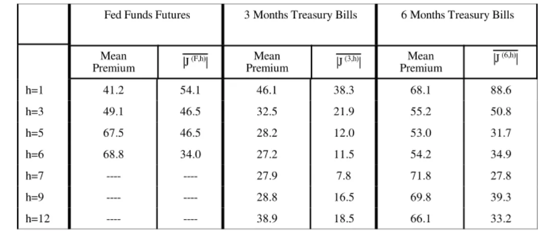
Our main result is that, above the effect of business cycles on risk premia, fluctuations in market belief have significant independent effect on the time variability of risk premia. We study the premia on long positions in Federal Funds Futures, 3-month and 6-month Treasury Bills. The annual mean risk premium on holding such assets for 1-12 months is about 40-60 basis points and we find that, on average, the component of market belief in the risk premium exceeds 50% of the mean. Since time variability of market belief is large, this component frequently exceeds 50% of the mean premium. This component is larger the shorter is the holding period of an asset and it dominates the premium for very short holding returns of less than 2 months. As to the structure of the premium we show that when the market holds abnormally favorable belief about the future payoff of an asset the market views the long position as less risky hence the risk premium on that asset declines. More generally, periods of market optimism (i.e. “bull” markets) are shown to be periods when the market risk premium is low while in periods of pessimism (i.e. “bear” markets) the market’s risk premium is high. Fluctuations in risk premia are thus inversely related to the degree of market optimism about future prospects of asset payoffs. This effect is strong and economically very significant.
JEL classification: C53, D8, D84, E27, E4, G12, G14.
Key Words: Rrisk Premium, market belief, perception models, empirical distribution, asset pricing
0. Introduction
Market risk premia vary over time and their fluctuations are a major cause of asset price volatility. But what drives changes in risk premia? The standard rational expectations answer relates changes in risk premia to changes in information about exogenous fundamentals which correctly alter the market’s assessment of future risky events, the most important of which are business cycles. Such a view implies that excess returns are predictable by changes in observed fundamentals which, in turn, explain market volatility. Although there is some empirical support for this view, it cannot be the full explanation. Asset prices are not explained well by fundamental factors and, as Paul Samuelson used
---* This research was supported by a grant of the Smith Richardson Foundation to the Stanford Institute for Economic Policy Research (SIEPR). We thank Robert Bliss for providing us with data, routines and documentation to compute zero coupon rates. We also thank Marco Aiolfi, Wen Chung Guo, Peter Hammond, Ken Judd, Stephen Morris, Hiroyuki Nakata, Carsten Nielsen, John O’Leary and Ho-Mou Wu for helpful discussions of the ideas of this paper and to Min Fan for extensive technical assistance and helpful comments on an earlier draft. Songtao Wang was helpful in detecting an error in Appendix B.
to quip, the market has forecasted nine of the last five recessions.
An alternative perspective holds that, in addition to exogenous fundamental conditions, the bulk of asset returns’ volatility is caused by fluctuations in market beliefs. We hold the view that agents do not know the true economic dynamics since it is a non-stationary system with time varying structure that changes faster than can be learned with precision from data. With diverse beliefs, a large fraction of price volatility is then endogenously generated. This component is called Endogenous Uncertainty. Papers reflecting these ideas include Harrison and Kreps (1978), Varian (1985), (1989), Harris and Raviv (1993), Detemple and Murthy (1994), Kurz (1974), (1994), (1997), (2008), (2009) Kurz and Beltratti (1997), Kurz and Motolese (2001), Kurz and Schneider (1996), Kurz and Wu (1996),
Motolese (2001), (2003), Nakata (2007), Nielsen (1996), (2003), (2011), Wu and Guo (2003), (2004), Guesnerie and Jara-Moroni (2011), Guo, Wang and Wu (2011). On monetary policy and aggregate fluctuations see Kurz Jin and Motolese (2005b), Branch and Evans (2006), (2011), Branch and McGough (2011), De Grauwe (2011), Wieland and Wolters (2011). On equity premium see Kurz and Motolese (2001) and Kurz Jin and Motolese (2005a). However, our earlier papers study risk premia via
simulations. They do not study determinants of risk premia either analytically or empirically.
In this paper we study the effect of market belief on the structure of risk premia. Beliefs are diverse but individually rational in a sense to be defined. Our problem is to establish the relation between market belief and market risk premia. We derive analytic results which are then tested empirically by using data on the market distribution of beliefs. Observations on market belief are extracted from data on monthly forecasts of future interest rates and macro economic variables compiled by the Blue Chip Financial Forecasts (BLUF) since 1983. A market state of belief is a distribution of individual beliefs and in the theoretical and empirical analysis we focus on the first two moments. Since an agent’s perceived risk premium is the conditional expectation of excess returns of an asset, an economy where agents hold diverse beliefs has many subjectively perceived risk premia.
The literature on excess returns and risk premia is large. We mention a few papers which report on convincing evidence gathered in recent years against the expectations hypothesis (e.g. Fama and Bliss (1987), Stambaugh (1988), Campbell and Shiller (1991), Cochrane and Piazzesi (2005) and Piazzesi and Swanson (2004)). They show that investments in Treasury securities generate predictable excess returns. Cochrane and Piazzesi (2005) exhibit predictable excess holding returns in bond markets
while Piazzesi and Swanson (2004) find excess returns in two futures markets: Fed Funds futures in 1988:10 - 2003:12 and Eurodollar futures in 1985:Q2-2003:Q4. “Predictability” is used here in the sense of exhibiting long term statistical correlation between current information and future excess returns. Cochrane and Piazzesi (2005) and Piazzesi and Swanson (2004) do not estimate structural models to explain the source of excess returns but deduce such returns from estimated reduced form models for forecasting returns. Broadly speaking, they argue that bond excess returns are associated with business cycles and for this reason they use pro-cyclical variables such as current yields or year over year growth rate of Non Farm Payroll (in short NFP) to predict excess returns.
There is a large literature in empirical finance that is compatible with our approach and which uses measures of market belief to forecast returns. A sample includes Miller (1977), DeLong et al. (1990), Lee et al.(2002), Diether et al.(2002), Johnson (2004), Park (2005), Baker and Wurgler (2006) and Campbell and Diebold (2009). Also, models with diverse beliefs have become the basis for recent work in Behavioral Finance. The literature in empirical finance cited mostly searches for measures to be used to forecast returns, and this is definitely not our aim. From a theoretical perspective the cited literature always takes the view that diverse beliefs reflect irrational behavior. Hence, the Behavioral Finance perspective is compatible with the Noise Trading view proposed by DeLong et al.(1990), and a Noise Trading view is the universal theoretical basis for the above literature in empirical finance. Our approach is to outline a theory of rational diverse beliefs and deduce from it empirical implications which can then be tested with market data. The present paper carries out this program.
To clarify the theoretical clash involved we note that in a Noise Trading world there are smart traders who know the truth and not-so-smart traders who trade aimlessly. Equilibrium reflects both the truth and the noise. We are not aware of any data on noise trading or on agents who declare themselves as noise traders. Hence, in our view noise trading theory cannot be falsified with data. In contrast, our theory proposes all traders are smart but lack knowledge of the true stochastic market dynamics. The true dynamics is time varying and due to complexity cannot be learned by anyone. Since investors know only empirical distributions deduced from data, equilibrium asset prices are determined only by what traders believe and by what they know. The true dynamics is irrelevant to asset pricing except for the way it reveals itself in the data agents know. Thus, lack of full knowledge of the truth is the foundation of belief diversity but rational diversity is not noise; it has a structure and can be studied scientifically.
Our results confirm earlier results about the effect of cyclical variables on risk premia. However, using our perspective we show that risk premia contain a large component generated by the dynamics of market belief. The market belief index is a state variable reflecting investor’s perceived future returns, net of fundamental information. This state variable functions like any fundamental variable and should be considered an externality taken as given by all. In equilibrium, fluctuations in market belief cause large changes in risk perception of market traders. Here we study the risk premia on the holdings of long positions in Federal Funds Futures, 3-month and 6-month Treasury Bills. The annualized mean risk premium on holding such assets for 1-12 months is about 40-60 basis points and we find that, on average, the component of market belief in the risk premium exceeds 50% of the mean. Since the time variability of market belief is large, this component is frequently larger than 50% of the mean premium. We find that this component is larger the shorter is the holding period of an asset.
We focus on two sets of results. First we show analytically and empirically that much of the time variability of market risk premium is generated endogenously by the dynamics of beliefs. Second, we show that the effect of market belief on the risk premium takes a specific form. When the market holds abnormally favorable belief about future payoffs of an asset the risk premium on long positions of that asset falls. More generally, market optimism about future economic conditions lowers the risk premium while pessimism about future economic conditions increases it. This inverse relationship suggests that important components of “bull” market in an asset class are likely to be abnormally favorable market beliefs which lower risk premia on long positions during such periods. We test our conclusions empirically in all three markets and find the data supports the theoretical findings.
1. Asset Pricing Under Heterogenous Beliefs 1.1 An Illustrative Decision Model
Consider an asset or a portfolio of assets whose market price is , paying an exogenous riskypt sequence {Dt,t'1,2,...} under a true and unknown probability which is non-stationary due toˆΠ structural changes over time. Let be the riskless interest rate, rt Rt'1%rt and hence excess return over the riskless rate is (1/pt)(pt%1%Dt%1&Rtpt). The risk premium over the riskless rate is the conditional expectations of excess returns. Since it is a function of equilibrium prices, a risk premium - as a function of state variables - is best deduced from equilibrium prices. With this in mind, the model below is used
1
We always have finite data and cannot estimate with certainty the measure on sequences. However, if this measure has a simple representation such as a Markov transition function, then with adequate data it can be approximated so closely as to make the assumption in the text entirely reasonable. Estimation of with an epsilon error only increases belief divergencemˆ as it reduces the scope of what is common knowledge and complicates the theory without adding much empirical substance.
2
It would be more realistic to assume the values Dt grow and the growth rate of the values has a mean μ rather than
the values themselves. This added realism is useful when we motivate the empirical model later but is not essential for the
to deduce a closed form solution of the asset price so as to enable a study of the factors determining the risk premium. To obtain closed form solutions we use a model which is very common in the literature on Noisy Rational Expectations Equilibrium (e.g. Brown and Jennings (1989), Grundy and McNichols (1989), Wang (1994), He and Wang (1995), Allen, Morris and Shin (2006) and others cited in
Brunnermeier (2001)). Nevertheless, our key results are fully general and do not depend upon the specific model used. We now address a key issue. Our agents do not know the true probability andˆΠ hold diverse probability beliefs about it. The fact that there are many subjective risk premia in the market raises two questions that will be at the basis of our development in the next two sections. First, why do agents not know the probability ? Second, what is the common knowledge basis of all agentsˆΠ in an economy with diverse beliefs?
Starting with the second question, our answer is past data on observables. The economy has a set of observable variables and Dt is one of them. Agents have a long history of the variables, allowing rich statistical analysis which leads all of them to compute the same empirical moments and the same finite dimensional distributions of the observed variables. Using standard extension of measures they deduce from the data a unique empirical probability measure on infinite sequences denoted by . It canˆm be shown that is stationary (see Kurz (1994)) and we call it “the stationary measure.” This is theˆm
empirical knowledge shared by all agents1. We assume the data reveals that under ˆm D
t, t'1,2,...
constitutes a Markov process where Dt%1is conditionally normally distributed with means μ%λd(Dt&μ)
and variance σ22. is the unconditional mean of . The unique probability is then known to all.
d μ Dt ˆm
To simplify define dt' Dt& μ, hence the process {dt,t'1,2,...} is zero mean with unknown true probability Π and an empirical probability m. Why is m not equal to Π? With this issue in mind we turn to the first question.
Our economy is undergoing changes in technology and social organization. These are rapid with major economic effects, making {dt,t'1,2,...} a non-stationary process. Although this means that the
distributions of the ‘s are time dependent, it is more than viewing {dt dt,t'1,2,...} as a sequence of productivity “regimes.” It also means that, although we measure the in a single unit of account, overdt time the nature of assets and commodities change. Such variability makes it impossible to learn the unknown Π. The probability m is merely an average over an infinite sequence of regimes, reflecting only long term frequencies. Belief diversity starts with the fact that agents disagree over the meaning of public information. They believe Π is different from m and construct models to express the
implications they see in the data. Being common knowledge, the empirical probability m is a reference for any concept of rationality. An agent’s model may be viewed as “extreme” but it cannot be declared “irrational” unless proved to contradict the empirical evidence. Thus, belief rationality requires a subjective model not to contradict the empirical evidence m.
Turning now to our infinite horizon model, at date t agent i buys shares of stock andθit receives the payment dt%μ for each of θit&1 held. We assume the riskless rate is constant over time so that there is a technology by which an agent can invest the amount Btiat date t and receive with certainty the amount BtiRat date t+1. The definition of consumption is then standard
. cti ' θit&1[pt% dt% μ] % B i t&1R& θ i tpt& B i t
Equivalently, define wealth Wti'cti%θ and derive the familiar transition of wealth
i tpt%B i t (1a) Wt%1i '(Wti&c . i t )R%θ i tQt%1 , Qt%1'pt%1%(dt%1%μ )&Rpt
are excess returns. Given some initial values the agent maximizes the expected utility
Qt (θi0, W i 0) (1b) U ' Eti (θi, ci) [j 4 s' 0&β t%s&1e&( 1 τc i t%s) | Ht]
subject to a vector of state variables and their transitions, all specified later. ψit Ht consists of all past observable variables. We recognize the limitations of the exponential utility and use it as a good vehicle to explain the main ideas, hence the term “illustrative” in this Section’s title. After deducing the closed form solution of equilibrium risk premium we show how to generalize the key results.
We now state an assumption and a conjecture. First, we assume the agent believes the payoff {dt,t'1,2,...} is conditionally normally distributed. Second, we conjecture that given the economy’s state variables, equilibrium price is also conditionally normal. In the next section we describe thept state variables and the structure of belief and Theorem 2 confirms the conjecture. In Appendix B we
show that for an optimum of (1a)-(1b), there is a constant vector u so the stock demand function is (2) θit(pt) ' . Rτ r ˆσ2Q[ E i t( Qt%1)% uψ i t]
is an adjusted conditional variance (see Appendix B for details) of excess stock returns which is ˆ
σ2Q
assumed constant and the same for all agents. The term uψit is the intertemporal hedging demand which is linear in agent i’s state variables. We have earlier assumed the dynamics of payoffs deduced from the
empirical frequencies is characterized by a first order Markov process with transition
(3) .dt%1 ' λddt % ρ d t%1 , ρ d t%1- N(0 , σ 2 d)
Since the implied stationary probability is denoted by m, we write Em[d .
t%1|dt]' λddt
Is the stationary model (3) the true data generating process? Those who believe the economy is stationary accept (3) as the truth. Such belief is rational since there is no empirical evidence against it. However, since {dt, t'1,2,...} is non-stationary with unknown probability Π, most agents do not believe (3) is adequate to forecast the future. All surveys of forecasters show that subjective judgment about the data contributes more than 50% to the final forecast (e.g. Batchelor and Dua (1991)). Hence, agents form their own beliefs about dt+1 and other state variables explored later. With possibly complex beliefs, how do we describe an equilibrium? For such a description do we really need to give a full, detailed, development of the diverse theories of all agents? The structure of belief is our next topic.
1.2 Modeling Heterogeneity of belief I: Individual Belief as a State Variable
The theory of Rational Beliefs due to Kurz (1994), (1997) defines an agent to be rational if his model cannot be falsified by the data and if simulated, its simulated data reproduce the stationary probability m deduced from the actual market data. The objective of this paper is the empirical test of Theorem 3 stated below and for that we use only the most basic restrictions the theory of Rational Beliefs imposes. Before explaining them we note that one of the theory’s aims is to account for the evidence of persistent belief diversity. But this diversity raises a methodological question. In
formulating an asset pricing theory should we describe in detail the subjective models of each of the N agents in the economy? With wide diversity this is a formidable task. Also, if the objective is to study dynamics of asset prices, is such a detailed description necessary? An examination of the subject reveals that, although an intriguing question, such a detailed task is not needed. Instead, to describe an
transition functions of state variables. Once specified, the Euler equations are fully defined and market clearing leads to equilibrium pricing. We now explain this observation.
In markets with heterogenous beliefs samples of individual forecasts are taken regularly and their distributions become publicly available. We then make the realistic assumption that forecast distributions are public observations over time. This fact points to the crucial difference between markets with and without private information. A market with asymmetric private information is secretive: agents do not reveal their forecasts since these provide real information about unobserved state variables. Such revelation eliminates the small advantage that each agent has relative to others. When an individual’s forecasts of a state variable are revealed in our market - without private
information - others do not view such forecasts as new information. They view them as an expression
of his opinion and consequently do not update their own beliefs about that state variable. Here a
forecaster uses the forecasts of state variables by other agents only to alter his forecasts of future endogenous variables since we shall show that these depend upon future market belief. But then, how do we describe the individual and market beliefs?
The key analytical step taken (see Nielsen (1996), Kurz (1997), Kurz and Motolese (2001), Kurz, Jin and Motolese (2005a),(2005b)) is to treat individual beliefs as primitive state variables, reflecting the characteristics of the agents. Here we use the approach of Kurz, Jin and Motolese (2005a), (2005b) as adapted and applied to the problem of this paper. We outline it now.
An individual belief about an economy’s state variable is described with a personal state of belief which uniquely pins down the transition function of the agent’s belief about next period’s
economy’s state variable. Hence, personal state variables and the economy-wide state variables are not
the same. A personal state of belief is like other state variables in the agent’s decision problem but is analogous to the concept of an agent “type.” A personal state of belief at t identifies the agent type at date t. However, at t he is not certain of his future belief types which are determined by a transition of his personal state of belief. The distribution of individual states of belief, which is defined as “the market state of belief,” is then an economy-wide observable state variable whose moments play an important role. All moments could matter in equilibrium, but due to the exponential utility which we use, equilibrium endogenous variables depend only on the mean market states of belief. This will be generalized in the empirical work reported later. As noted, the crucial fact is that the market state of belief is observable. In equilibrium, endogenous variables (e.g. prices) are functions of the economy’s
state variables, including market state of belief. But in a large economy an agent’s “anonymity” implies that a personal belief state has a negligible effect on prices and past personal states are not observed. Finally, due to the effect of market belief on endogenous variables, an agent uses the equilibrium map to forecast all endogenous variables and for that he forecasts future market belief. To forecast future endogenous variables an agent must therefore forecast the beliefs of others. The main issue we need to discuss next is the dynamics of individual beliefs and for this we turn to rationality restrictions.
A direct implication of the Rational Belief principle says an individual belief cannot be a
constant transition unless an agent believes the stationary transition (3) is the truth. This is so since if
one holds a constant transition as his belief but not (3) then the time average of his belief is different from (3). Since (3) is the time average in the data, this proves the agent is irrational. We then make the key observation that rationality implies that beliefs must fluctuate and thus have inherent dynamics which induces a crucial component of market volatility that we call “Endogenous Uncertainty.”
Given the extensive evidence for persistent diverse beliefs which cannot be (3), one concludes agents hold wrong beliefs. But being rational and “wrong” are not in conflict. Rational agents hold wrong beliefs when there is no empirical proof they are wrong. Indeed, when agents use diverse models when there is only one true law of motion, then most are wrong most of the time and market forecasts are often wrong. The term “wrong” is used relative to an unknowable standard. Market “mistakes” deduced from rational behavior are then at the heart of our theory of market volatility. Since rationality requires beliefs to reproduce the data and not deviate from it consistently, we use this rationality restriction to require the belief index (presented next) to have an unconditional mean zero.
We now introduce agent i’s state of belief gti. It describes his perception by pinning down his transition functions. Adding to “anonymity” we assume agent R knows his own and the marketgtR
distribution of gti at t across i. In addition he observes past distributions of the gτi for all τ < t hence he knows past values of all moments of the distributions of gτi. We specify the dynamics of gti by
(4) gt%1i ' λZg
i t % ρ
ig
t%1 , ρigt%1- N(0 , σ2g)
where ρigt%1 are correlated across i reflecting correlation of beliefs across individuals. The concept of an individual state of belief is central to our development and we consider (4) to be a primitive. It is simply a positive description of type heterogeneity which can be justified in many ways. One compelling reason for it is that it is supported by the data as shown later. Analytic justifications can also be
How is gti used by agent i? If dt%1i denotes agent i’s perception of t+1 payoff then gtipins down his expectation Eti[dt%1i &λddt] of the difference between his date t forecast of all state variables and the forecasts under the empirical distribution m. Hence, agent i’s date t perceived distribution of dt%1is
(5) dt%1i ' λddt % λ . g dg i t % ρ id t%1 , ρidt%1- N(0 , ˆσ2d)
The assumption that is the same for all agents is made for simplicity. It follows that measuresσˆ2d gti
(6) Ei[di . t%1|Ht,g i t ] & Em[dt%1| Ht]' λ g dg i t
As explained before, restricting gti to have a zero unconditional mean follows from the Rational Belief principle. But (6) also shows how to measure gti in practice. For a state variable Xt, data on i’s forecasts of Xt+1 (in (5) it is dt%1 ) are measured by Ei[X . One then uses standard
i t%1|Ht,g
i t ]
econometric techniques to construct the stationary forecast Em[X used to compute (6). Such
t%1| Ht]
construction and the data it generates are used by Fan (2006). An agent who believes the empirical distribution is the truth is described by gti ' 0. He believes dt%1-N(λddt,σ . Since a belief is about
2 d)
our changing society, gti reflect belief about different economies. For example, in 1900 the gti were related to electricity and combustion engines, while in 2000 they reflected beliefs about information technology. Hence, success or failure of past gτi tell you little about what present day gti should be.
1.3 Modeling Heterogeneity of belief II: Individual and Market Beliefs
Averaging (4) denote by the mean of the cross sectional distribution of Zt gti and we refer to it as “the average state of belief.” It is observable. Due to correlation across agents, the law of large numbers is not operative and the average of ρigt over i does not vanish. We write it in the form
(4b) Zt%1 ' λZZt % ρ .
Z t%1
The true distribution of ρZt%1 is unknown. Correlation across agents exhibits non stationarity and this property is inherited by the { Zt , t = 1, 2, ...} process. Since Zt are observable, market participants have data on the joint process {(dt, Zt) , t' 1,2,. ..} hence they know the joint empirical distribution of these variables. For simplicity we assume that this distribution is described by the system of equations
(7a) dt%1 ' λddt % ρ d t%1 (7b) Zt%1 ' λZZt % ρ Z t%1 ρdt%1 ρZt%1 - N 0 0, σ2d, 0, 0, σ2Z ' ˜Σ , i.i.d.
Now, an agent who does not believe that (7a)-(7b) is the truth, formulates his own model\belief. We have seen in (5) how agent i’s belief state gti pins down his forecast of dt%1i . We now broaden this
idea to an agent’s perception model of the two state variables (dt%1i , Zt%1i ). Keeping in mind that before observing (dt%1,Zt%1) agent i knows dt and Zt, his belief takes the general form
(8a) dt%1i ' λddt % λ g dg i t % ρ id t%1 (8b) Zt%1i ' λZZt % λ g Zg i t % ρ iZ t%1 ρidt%1 ρiZt%1 ρigt%1 - N 0 0 0 , ˆ σ2d, ˆσZd, 0 ˆ σZd, ˆσ 2 Z, 0 0 , 0 , σ2g , ' Σi (8c) gt%1i ' λZgti % ρigt%1
(8a)-(8b) show that, as required, gti pins down the transition of both state variables (dt%1i ,Zt%1i ). This simplicity ensures that one state variable pins down agent i’s subjective belief of how conditions at date t are different from normal as reflected by the empirical distribution:
Eti dt%1 Zt%1 & E m t dt%1 Zt%1 ' λgdg i t λgZg i t .
Note: in (8a)-(8c) the random term is not required to be i.i.d. Also, we used the minimal restrictions implied by rationality which we need for Theorem 3. Detailed rationality conditions, which imply the average of (8a)-(8c) yield (7a)-(7b) are not used explicitly here and are explained in Appendix A.
Is belief heterogeneity central to (8a)-(8c)? Given the exponential utility, only average market belief matters so why could the model not be reduced to a representative agent? The answer is seen in Equation (8b). A crucial element of the theory is that each agent forecasts future market belief and for that an agent must perceive the market as different from himself. If an agent identifies himself with the average market then there is nothing to forecast and (8b) is the same as (8c). Market heterogeneity also reveals that the dynamics of depends crucially upon the correlation across agents’ beliefs ratherZt than on their beliefs. Since this correlation is not determined by individual rationality aggregate dynamics is a consequence of heterogeneity and not of any individual rationality principle.
The average market expectation operator is defined by ¯Et(C) ' 1 . From (8c) it is N j N i Eti(C) . ¯Et dt%1 Zt%1 & E m t dt%1 Zt%1 ' λgdZt λgZZt
Higher Order Beliefs. One must distinguish between higher order belief which are temporal and those which are contemporaneous. Within our theory the system (8a)-(8c) defines agent i’s probability over sequences of (dt, Zt, gti)and as is the case for any probability measure, it implies temporal higher order beliefs of agent i with regard to future events. For example, we deduce from (8a)-(8c) statement like
. Eti(dt%N)'EtE i t%1.. .E i t%N&1(dt%N) , E i t (Z i t%N)'EtE i t%1. ..E i t%N&1( Z i t%N)
It is thus clear that temporal higher order beliefs are properties of conditional expectations. In addition, by (8c) (or equivalently (4)) we have ¯Et(dt%N%1)'λd¯Et(dt%N)%λ . Hence we can also deduce
g
d¯Et(Zt%N)
perceived higher order market beliefs by averaging individual beliefs. For example, we have that
. ¯Et(Zt%N) ' ¯Et¯Et%N&1(dt%N) & ¯EtEt%N&1m (dt%N)
The perception models (8a)-(8c) show that properties of conditional probabilities do not apply to the market belief operator ¯Et(C) since it is not a proper conditional expectation. To see why let
be a space where take values and Gi be the space of . Since i conditions on , his
X'D×Z (dt, Zt) gti gti
unconditional probability is a measure on the space where (( D× Z× Gi)4,öi) öi is a sigma field. The market conditional belief operator is an average over conditional probabilities, each conditioned on a
different state variable. Hence, this averaging does not permit one to write a probability space for the
market belief. The market belief is neither a probability nor rational and we have the following result:
Theorem 1: The market belief operator violates iterated expectations: ¯Et(dt%2) … ¯Et¯Et%1( dt%2).
Proof: Since Eti(dt%2)' λdE it follows that
i t( dt%1)% λ g dE i t(g i t%1)' λd[λddt%λ g dg i t ]% λ g dλZg i t (9) ¯Et(dt%2)' λ2ddt%λ . g d(λd% λZ) Zt
On the other hand we have from (8a) that ¯Et%1( dt%2)' λddt%1 % λ hence we have that
g dZt%1 . Eti¯Et%1( dt%2)' λd[λddt% λ g dg i t ]% λ g d[λZZt% λ g Zg i t ]
Aggregating now we conclude that
(10) ¯Et¯Et%1(dt%2)' λ2ddt% λ .
g
d(λd% λZ% λ g Z) Zt
Comparison of (9) and (10) shows that ¯Et(dt%2) … ¯Et¯Et%1( dt%2).
Belief and information: understanding . For each agent, is a state variable like others. NewsZt Zt about are used to forecast prices as GNP growth is used to assess recession risk. Market belief mayZt be right or wrong and risk premia may rise or fall just because agents have more or less favorable views about the future, not necessarily because there is data to convince investors the future is bright or bleak. But then, how do they update beliefs given data on ? In contrast with private information, agents doZt not revise their beliefs about the state variable dt%1: (8a) specifically does not depend upon . They doZt not view as information aboutZt dt%1 since it is not a “signal” about unobserved private information
they do not have. Indeed, they know all use the same public information. However, is crucial “news”Zt about what the market thinks aboutdt%1! The importance of is it’s value in forecasting endogenousZt variables. Date t endogenous variables depend upon and since market belief exhibits persistence,Zt agents use today’s market belief to forecast future endogenous variables. How is this equilibriated?
1.4 Combining the Elements: the Implied Asset Pricing Under Diverse Beliefs
We now derive equilibrium prices and the risk premium. For details see Appendix B where we also explain the term σˆ2Q, which is the “adjusted” conditional variance of Qt%1. We have also explained in 1.3 why the state variables in (2) are specified by the vector ψit' (1, dt,Zt,g . Hence, rewrite (2) as
i t) (11) θit(pt) ' . Rτ r ˆσ2Q[ E i t( Qt%1) % uψ i t] , u'(u0, u1, u2, u3) , ψ i t ' (1,dt, Zt,g i t )
For an equilibrium to exist we need some stability conditions. First we require the interest rate r to be positive, R = 1 + r > 1 so that 0 < 1 . Now we add:
R< 1
(12) Stability Conditions: We require that 0 < λd < 1 , λZ < 1 , 0 < λZ % λ .
g Z < 1
The first requires {dt , t = 1, 2, ...} to be stable and have an empirical distribution. The second is a stability of belief condition. It requires i to believe(dt, Zt) is stable. To see why, take expectations of (8b), average over the population and recall that Zt are market averages of the g . This implies that
i t
(13) ¯Et[Zt%1] ' (λZ % λ .
g Z)Zt
Theorem 2: Consider the model with heterogenous beliefs under the stability conditions specified with supply of shares which equals N. Then there is a unique equilibrium price function which takes the form
. pt' addt % aZZt % P0
Proof: Average (11), use the fact that the aggregate stock supply is N and rearrange to have
(14) r ˆσ .
2 Q
Rτ ' [ ¯Et(pt%1%dt%1%μ ) & Rpt% (u0%u1dt%(u2%u3)Zt) ]
Now use the perception models (8a)-(8b) about the state variables, average them over the population and use the definition of Zt to deduce the following relationships which are the key implications of
(15a) ¯Et(dt%1 % μ ) ' λddt % μ % λgdZt
(15b) ¯Et[Zt%1]' (λZ%λ
g Z)Zt
Using these to solve for date t price we deduce
(16) pt ' 1 R[ ¯Et(pt%1)]% 1 R[ (λd% u1)dt% (λ g d% u2% u3)Zt]% 1 R[ μ% u0]& rˆσ2Q R2τ
(16) shows that equilibrium price is the solution of a linear difference equation in the two state
variables (dt , Zt). Hence, a standard argument (see Blanchard and Kahn(1980), Proposition 1, page 1308) shows that the solution is
(17a) pt' addt % aZZt % P0
To match coefficients use (17a) to insert (15a) - (15b) into (16) and conclude that
(17b) ad ' λd% u1 . R & λd (17c) aZ ' ( ad% 1)λ g d% (u2% u3) R&(λZ%λ g Z) (17d) P0 ' (μ % u0) . r & ˆ σ2Q Rτ
The stability conditions ensure that (17a) - (17d) is the unique solution as asserted.
Since we do not have a closed form solution for the hedging demand parameters u'(u0,u1,u2,u3) we computed numerical Monte Carlo solutions. For all values of the model parameters given the interesting case (λgd> 0,λ we find and . These are reasonable conclusions: increases with
g
Z> 0) ad>0 aZ>0 pt
higher and with higher - today’s market belief in unusually higher future dividends.d t Zt
1.5 Equilibrium Risk Premium Under Heterogenous Beliefs 1.5.1 The Main Equilibrium Results
Under heterogenous beliefs we have diverse concepts of risk premia and one chooses a concept which is appropriate for an application. The risk premium on a long position, as a random variable, is (18) πt%1 ' pt%1 % dt%1 % μ & Rpt.
pt
(18) is a random variable measuring actual excess returns of stocks over the riskless bond. The need is to measure the premium as a known expected quantity, recognized by participants. We have three such measures. The first is the subjective expected excess returns by agent i, computed by using the
equilibrium map (17a) and the perception model (8a) -(8c) to show that (19) 1 ptE i t(pt%1%dt%1%μ&Rpt)' 1 pt[(ad%1)(λddt%λ g dg i t)%aZ(λZZt%λ g Zg i t)%μ %P0&Rpt]
Aggregating over i, the market premium is the average market expected excess returns. This perceived premium reflects what the market expects, not what it receives. From (19) it is measured by
(20) 1 pt ¯Et(pt%1 % dt%1 % μ & Rpt) ' ' 1 pt[(ad%1)(λddt%λ g dZt)% aZ(λZZt% λ g ZZt)%μ %P0&Rpt]
Neither (19) nor (20) are objective risk premia. We thus turn to an objective measure, common to all agents, computed by agents studying the long term time variability of the premium and measuring it by the empirical distribution of (18). Using (17a) and the stationary transition (7a)-(7b) we have
(21) Etm[πt%1]' 1 ptE m t [pt%1%dt%1%μ &Rpt]' 1 pt[( ad%1)(λddt)%aZ(λZ)Zt%μ %P0&Rpt] Observe that (21) is the way Econometricians and all researchers cited above have measured the risk premium. For this reason we refer to it as “the” risk premium.
We arrive at two conclusions. First, the differences between the premia in (19) and (20) is
(22a) 1 . ptE i t(pt%1%dt%1%μ&Rpt)& 1 pt ¯Et( pt%1%dt%1%μ &Rpt)' 1 pt[(ad%1)λ g d% aZλ g Z]( g i t & Zt)
This says that from the perspective of trading, all that matters is the difference gti& Zt of individual from market belief. Also, the risk premium is different from the market perceived premium when Z …0.
(22b) 1 .
ptE
m
t (pt%1%dt%1%μ&Rpt)&
1
pt ¯Et( pt%1%dt%1%μ &Rpt)' & 1 pt[(ad%1)λ g d% aZλ g Z] Zt
The more important conclusion is derived by combining (20) with (22b). By (17c) we have , hence we can deduce the main result:
&(u2%u3)'&aZ( R&λZ)%[(ad%1)λ g d%aZλ
g Z]
Theorem 3:
The equilibrium risk premium has the following analytical expression(23a) 1 ptE m t (pt%1%dt%1%μ&Rpt)' 1 pt [( r ˆσ2Q
Rτ & u0& u1dt)& aZ(R& λZ) Zt] Since az > 0, R > 1 and λZ< 1 it follows that
(23b) the Risk Premium Etm[πt%1] is decreasing in the mean market belief .Zt
Conclusions (23a) -(23b) are central to this paper. (23a) and the earlier results exhibit the Endogenous Uncertainty component of the risk premium which we call “The Market Belief Risk Premium.” It shows that market belief has a complex effect on market risk premia. The effect of belief consist of two parts
(I) The first is the direct effect of market beliefs on the permanent mean premium r ˆσ . It is
2 Q
shown in the Appendix that there exist weights (ω1,ω12,ω2) such that σˆ2Q' Var . i t((ω1(λddt% λ g dg i t %ω12ρ id t%1)%ω2(λZZt%λ g Zg i t %ω12ρ iZ t%1))
Volatility of individual and market belief, which we call “Endogenous Uncertainty” contributes directly to the volatility of excess returns and increases permanently the risk premium.
(II) The second is the effect of market belief on the time variability of the risk premium, reflected in & aZ(R& λZ) Zt with a negative sign when Zt > 0.
To explain this second result we note that it says that if one runs a regression of excess returns on the observable variables, the effect of the market belief on long term excess return is negative. This sign is surprising since when Zt > 0 the market expects above normal future dividends but in that case the risk premium on the stock is lower. When Zt < 0 the market holds bearish belief about future dividend but the risk premium is higher. Since we have data on Zt and on the distribution of belief the result will be empirically tested. Before proceeding to the empirical test we discuss some ramifications of this result.
1.5.2 The Market Belief Risk Premium is Fully General
The main result (23b) was derived from the assumed exponential utility function. We argue that this result is more general and depends only on the positive coefficient az of in the price map. ToZt show this, assume any additive utility function over consumption and a risky asset which pays a
“dividend” or any other random payoff . Denote the price map by dt pt ' Φ(dt, Zt). We are interested in the slope of the excess return function Etm[πt%1] with respect to . Focusing only on the numeratorZt
, linearize the price around 0 and write . The Etm[ pt%1 % dt%1 % μ & Rpt] pt ' Φddt % ΦZZt %Φ0 desired result depends only upon the condition ΦZ> 0. It is reasonable as it requires current price to increases if the market is more optimistic about the asset’s future payoffs. To prove the point note that Etm[ pt%1%(dt%1%μ)&Rpt]. E
m
t [Φddt%1%ΦZZt%1%Φ0%(dt%1%μ)&R(Φddt%ΦZZt%Φ0)]
' [(Φd%1)λd& RΦd]dt&ΦZ(R& λZ)Zt%[μ %Φ0( 1&R)]. The desired result follows from the fact that ΦZ> 0, R > 1 and λZ< 1.
The price map might be more complicated. If we write it as pt ' Φ(dt, Zt, Xt) where X are other state variables (in particular, the distribution of wealth), the analysis is more complicated since we need to specify a complete model for forecasting Xt%1 but the main result continues to hold.
1.5.3 Interpretation of the Market Belief Risk Premium
Why is the effect of Zt on the risk premium negative? Since this result is general and applicable to any asset with risky payoffs, we offer a general interpretation. Our result shows that when the market holds abnormally favorable belief about future payoffs of an asset the market views the long position as less risky and consequently the risk premium on the long position of the asset falls. Fluctuating market belief implies time variability of risk premia but more specifically, in the long run fluctuations in risk premia are inversely related to the degree of market optimism about future prospects of asset payoffs.
To explore the result, it is important to explain what it does not say. One could interpret it to confirm a common claim that to maximize excess returns it is optimal to be a “contrarian” to the market consensus. To understand why this is a false interpretation note that when an agent holds a belief about future dividends, the market belief Zt does not offer him new information to alter his belief about dividends. If the agent believes future dividends will be abnormally high but Zt< 0, the agent
does not change his forecast of dt%1. He uses Zt only to forecast future prices. Hence, Zt is a crucial input to forecasting returns without changing the forecast of dt%1. Since given the available information and his probability belief, which is, say, an optimizing agent is already on his demand function. HeΓi
does not just abandon his demand by replacing with the empirical measure m. This argument isΓi
analogous to the one showing why it is not optimal to adopt the log utility as your utility even though it maximizes the growth rate of your wealth. Yes, it does that, but you dislike the sharp declines which you expect to occur in the value of your assets if you follow the strategy called for by the log utility. By analogy, following a “contrarian” policy implies a high long run average return in accord with m since this is what (23a) says. But if your subjective model disagrees with the probability m you will dislike being short when your optimal position should be long. This argument explains why most people do not systematically bet against the market, as a “contrarian” strategy (23a) would dictate.
Taking a positive view, our results show that fluctuations in market belief are crucial for the time variability of the risk premium and the market pricing of risk. Market optimism in bull markets or pessimism in bear markets have drastic effects on market risk perception. A bull market is a market in
which risk perception is low and a bear market is one in which risk perception is high. Our result (23a)
shows that on average, market optimism induces lower risk premium and market pessimism generate high risk premium. But due to diverse beliefs the individually perceived premia are diverse. To see this
i
optimizing agents take into account information about in calculating their premia. From theirZt perspective the state variable is used to assess risk in the same way as NFP is used to assess the riskZt of recessions and hence the market risk premium. We turn now to an empirical test of our theory.
2. Testing of the Endogenous Time Variability of the Risk Premium: The Data 2.1 The Forecast Data
We use data on the distribution of commercial forecasts and take them as proxies for forecasts made by the general public. The data is circulated monthly by the Blue Chip Financial Forecasts (BLUF). It provides forecasts of over 50 economists at major corporations and financial institutions. The number of forecasters may vary from month to month and, due to mergers and other
organizational changes, the list of potential forecasters also changes over time. A sample of forecasters includes Moody's Investors Service, Prudential Securities, Inc. Ford Motor Company, Macroeconomic Advisers LLC, Goldman Sachs & Co., DuPont, J. P. Morgan Chase, Merrill Lynch, Fannie Mae, and others. BLUF reports forecasts of U.S. interest rates at all maturities along with forecasts of GDP growth and inflation. Forecasts reported in BLUF are collected on the 24th and 25th of each month and released to subscribers on the first day of the following month.
The BLUF publishes, for each variable, individual and mean (“consensus”) forecasts. The mean is taken over all forecasters participating in that month. Forecasts are made for several quarters into the future. For each horizon forecasters are asked to forecast the average value of that variable
during the future quarter in question. Note, the realized value of any variable for the quarter in which
forecasts are released is not known at forecasting time since such data is available only after the quarter ends. As a result, each set of forecasts includes “current quarter” forecast which is denoted by the horizon h = 0. Hence, h = 1 means “the quarter following the quarter in which the forecasts were made.” The BLUF publication was initiated in 1983:01 and circulated forecast data with horizons of h = 0,1,...,4 quarters. The initial version of the files provided data for the Fed Fund rate, 1-month Commercial Paper rate, 3-month T-Bill rate, 30-year Treasury Bonds rate, AAA long term corporate bonds rate, growth rates of GNP, changes in the GNP deflator and CPI. In 1988:01 the BLUF added individual and market mean forecasts to complete the yield curve on treasury securities covering also maturities of 6 months, 1 year, 2 years, 5 years and 10 years. In 1992:01 forecasts of GNP and GNP deflator were replaced by forecasts of GDP and GDP deflator. In 1997:01 the forecast horizon was
expanded by one quarter and from that date h = 0,1,...,5 quarters. Hence, a uniform panel data set for the term structure of interest rates is available starting in 1988:01. The data set has undergone other minor changes since its first release. These are not relevant to this paper and are not reported here.
In the empirical work we use a month as a unit of time. Hence, we had to translate quarterly mean forecasts to monthly forecasts. This was accomplished by an interpolation which selected for each t and for each variable the B-form of a least squares cubic spline piecewise polynomial which minimized the squared deviations from the given forecasts. When a variable is recorded monthly then all forecasters actually know at each date the realized monthly variable at hand for those months of the present quarter which have already past. This clearly applies to all interest rate data. Hence, it was useful to include in all interpolations past realized data of the variable in question for one quarter
before date t (hence, three monthly observations). This procedure improves continuity at date t. An
optimal polynomial is computed for each date and utilizes no future market data of any kind. At the end of the interpolation we have monthly data with monthly forecast horizons h=1,2,...,12.
The forecasts reported in BLUF are labeled by their release date, which is the start of each month. Hence, these forecasts are conditional on information available at the moment the forecasts were collected which is the end of the month previous to release. For example, data released in 1988:01 is recorded in our “sample period” as 1987:12 since the data released on January 1, 1988 is based on information available to forecasters at a date identified by us as 1987:12. Therefore all dates in this paper should be considered as identified with the end of the month. The data set has been updated in a format suitable for computations up to 2003:11.
2.2 Extracting Market States of Belief
The concepts of individual and market states of belief are central to the empirical work and we now explain how they are constructed. For any variable X denote by Eti{Xt%h} agent i’s conditional forecast of Xt%h at date t and by Etm{Xt%h} the forecast under the stationary probability m. Agent i’s state of belief about Xt%h is then defined by
. Z(X,h,i)t ' Eti{Xt%h}&Etm{Xt%h}
This expression removes from Z(X,h,i)t the effect of other state variables. Since Z(X,h,i)t is the deviation from the stationary forecast, it must be interpreted properly. Thus, suppose y is growth rate of GDP.
3 The data is publically available on Watson’s web page http://www.princeton.edu/~mwatson/publi.html
output will necessarily go up. He does believe output will grow faster than “normal,” defined by the growth rate expected under m. The market state of belief is defined by
Z(X,h)t ' 1 N j
N
i'1
[ Eti{Xt%h} & Etm{Xt%h} ] ' ¯Et{Xt%h} & E m
t {Xt%h}
and the cross sectional variance of beliefs is (σt(X, h))2' 1
Nj
N
i'1
[Eti{Xt%h}&Etm{Xt%h}]&[¯Et{Xt%h}&Etm{Xt%h}]2' 1 N j
N
i'1
Eti{Xt%h}& ¯Et{Xt%h}2. Since ¯Et{Xt%h}is the mean forecast, Z(X,h)t reflects the market’s views about economic conditions which are different at t from what is expected under m. These differences are the reason why the market forecasts ¯Et{Xt%h}and not Emt {Xt%h}. “Optimism” or “pessimism” depend upon the context. For example, Z(y,h)t > 0 means the market is optimistic about abnormally high output growth in t+h. If R(j) is j maturity interest rate, then Z(j ,h) means the market expects this rate to be higher than
t > 0
normal at t+h. The market belief about Fed Funds rates is a belief about future monetary policy. Hence, Z(F,h)t > 0 means the market expects an abnormally tight monetary policy. Note that in this paper, all belief variables are about future interest rates.
To measure Z(X,h)t we need data on the two components which define it. BLUF files provide direct data on Eti{Xt%h} and ¯Et{Xt%h}as discussed. We have monthly forecast data on interest rates at different maturities, GDP growth , change in the CPI and the GDP deflator. The key issue is thus the construction of the stationary forecasts Etm{Xt%h}. These forecasts are made with a model that takes into account all data that was available at date t hence we take into account the release date of each variable used in the following analysis. A feature of stationarity is time invariance, implying the model is valid out of sample. This is an idealization which we can only approximate, given the relatively limited data set which we have. We thus compute Etm{Xt%h}employing the Stock and Watson’s (1999), (2001), (2002), (2005) method of diffusion indices. We briefly explain this procedure.
We started with the Stock & Watson’s data set3 developed by Data Resources and Global Insight. It contains 215 monthly U.S. time series from 1959:01 to 2003:12, covering the main economic sectors. As discussed in Stock and Watson (2005), the series are transformed by taking logarithms and/or by differencing. First differences of logarithms (growth rates) are used for real quantity variables, first differences are used for nominal interest rates, and second differences of logarithms (changes in growth rates) for price series. Because of missing data we use (see Stock and
Watson (2005)) only 127 series from 1959:01 to 2003:12. These represent ten main categories of variables: consumption, employment, exchange rates, housing starts, interest rates, money aggregates, prices, real output, stock prices and the University of Michigan Index of Consumer Expectations. Stacking them, we obtain an information matrix of dimension 540 by 127. One of Stock and Watson’s (1999) conclusion is that effective time invariant models need to employ a small number of variables. The reason for this observation is that linear forecasting models with a large number of variables are unstable and forecast poorly out of sample. The Stock-Watson method reduces the rank of the matrix but keeps as much information as possible by creating diffusion indices constructed via principal component analysis to extract factors that best explain the variance of the information matrix.
For the period at hand the five greatest factors explain 43% of the variation in the information matrix and with twenty factors the variance explained is 74%. However, the marginal contribution of a factor declines rapidly implying that little marginal explanatory power is gained when using more than a few factors. Indeed, since we study interest rates which are rather persistent, nothing in this paper is changed by using more than four factors in the stationary forecasting scheme we adopt below. Stock and Watson (2002) concluded that a combination of factors and lags of the forecasted variable is the best information set. For any variable X the objective is to compute forecasts of
using information at time t. In all regressions of Section 3 we need stationary forecasts of market Xt%h
nominal interest rates and for these variables the forecasts are constructed as follows:
(i) let ΔxT%h'XT%h&XT denote the stationary h-period change in a nominal interest rate and FTi for denote the first four factors deduced from date T information matrix;
i'1,..., 4
(ii) estimate the parameters αˆh, ˆβh,i, ˆγhby the following OLS regression:
ΔxT%h ' αh ;
% j4
i' 1β h,iFi
T % γhΔxT % gT%h, for T ' 1,...,t&h
(iii) the forecasts of ˆΔxt%hat date t are then given by:
. ˆΔxt%h,t ' ˆαh % j 4 i' 1 ˆβ h,i Fti % ˆγhΔx t
Finally, the stationary forecasts of the interest rates are Etm{Xt%h} ' Xt % ˆΔxt%h,t. A similar procedure is used for the GDP deflator except that ΔxT%h'XT%h.
Real Time vs. A Single Estimate. Had our data set been very long, the stationary forecast
could be constructed from any long time interval and it would be time invariant. Since our Etm{Xt%h}
and are made by using real time forecasts. For each date in the sample we thus use Etm{Xt%h} Z(X,h)t
data from 1959:01 up to the given date in order to recompute the factor loadings, reestimate a stationary model with which we compute Etm{Xt%h} and then deduce the values of Z(X,h)t .
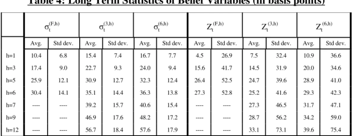
Table 1A: Summary Statistics of Market Beliefs h = 6 Months or 2 Quarters Ahead Time Average Standard Deviation Autocorrelation Fed Fund rate
1 year T-bill rate GDP deflator 0.273 0.238 0.365 0.528 0.429 0.595 0.700 0.735 0.674 h = 12 Months or 4 Quarters Ahead
Fed Fund rate 1 year T-bill rate GDP deflator 0.267 0.385 0.398 0.763 0.681 0.798 0.632 0.841 0.740
Tables 1A and 1B provide some summary statistics of a sample of extracted market belief variables Z(X,h)t . The last column in Table 1A reports the first order autocorrelation parameter. Although theory requires each market belief to have a long term time average equal to zero, it is clear the means over short time periods are not zero. Indeed, the fact that the belief indices for inflation and nominal interest rates have positive time averages for the period at hand is significant. It reflects the forecasting bias in the US during that era when beliefs in inflation and doubts about the efficacy of monetary policy persisted (see Kurz (2005)) despite the mounting evidence against these beliefs. Note also the autocorrelation coefficients which are compatible with the Markov dynamics of belief in (4).
Table 1B: Correlation Matrix of Market Beliefs 6 Months or 2 Quarters Ahead Fed Fund rate 1 year T-bill rate GDP deflator Fed Fund rate
1 year T-bill rate GDP deflator 1.000 0.850 0.363 1.000 0.298 1.000 12 Months or 4 Quarters Ahead
Fed Fund rate 1 year T-bill rate GDP deflator 1.000 0.856 0.516 1.000 0.523 1.000
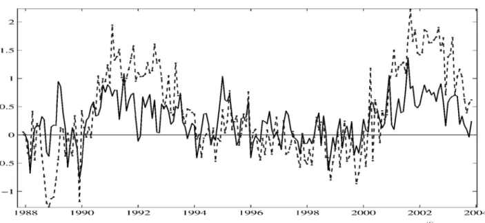
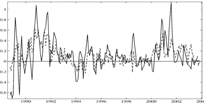
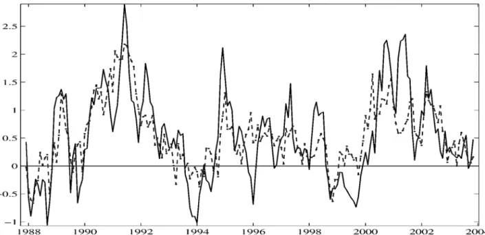
To illustrate, Figure 1 traces the graph of Z(6 ,h)t for the 6-months T-bill rate with horizons h = 4, 12. The figure shows the belief indexes exhibit large fluctuations ranging from -1.5% to +2.5%. which are very significant from the economic point of view. In Figure 2 we trace the time variability of the cross-sectional standard deviations σt(6, h)of the Z(6 ,h,i) across i, for horizons h = 4, 12. It is
t
clear from the figure that the dispersion of beliefs increases with the forecasting horizon. This is a common feature of all data on belief distributions.
2.3 Data on Realized Market Interest Rates, Rates of Return and Excess Returns
Treasury Bills market. Theory suggests we work with interest rates implied by zero coupon
bond prices hence we used data on zero coupon securities with maturities of 1 to 18 months, based Figure 2: 6-month Treasury Bill rate: 4 and 12(dashed line) month ahead standard deviation of Market Belief Zt(6)
4Traders are required to put up good faith security deposit which is a margin collateral to ensure they honor their pledge for the deposit as agreed. The collateral securities are owned by the parties to the contract who continue to benefit from any return to their investments. Margin cash is often held in the form of T Bills which yield interest to the owner. Hence a buyer or seller of a futures contract do not have any investment or opportunity cost except for the risk they take on the actual on the Fama-Bliss file (see Fama and Bliss (1987)). The data up to 2003:11 was generated by a FORTRAN routines (provided by R.R. Bliss), using a method developed by Bliss for the unsmoothed Fama-Bliss data set (see Bliss (1997)). Let π(j,h)t%h be the one period excess holding returns of T Bills with (j + h) maturity held for h periods and sold at maturity j. It can be measured as a monthly or an annualized rate since all we say here about T Bills is independent of the unit of time selected. We study the h - month excess holding returns defined by
hπ(j,h)t%h ' (j%h)R (j%h) t & jR (j) t%h& hR (h) t
where Rt(τ)is the one period interest rate implied by a zero coupon bond with maturity at τ. We study the two maturities j = 3 and 6 months. All data on the right hand side of the expression are then available in the Fama-Bliss file described above. The limiting factor in the study of this market is the BLUF data hence the period of analysis is 1987:12- 2003:11.
It is useful to clarify the trading mechanics needed to realize h period holding returns earned by selling a specified debt τ dates in the future. For example, to sell a six month Treasury Bill 12 month from now one must buy a Treasury Bond with maturity of 18 months and sell it 12 month from now. Returns on this long position consist of interest earned plus capital gains or losses realized.
Federal Fund Futures market. The second set of markets are for non contingent Federal
Funds futures contracts with diverse monthly settlement horizons. A Fed Funds futures contract enables buyers and sellers to trade the risk of the Fed Funds rate that would prevail at the time of settlement. Hence this is the risk of the future target of the Fed Fund rate that would be fixed by the Fed’s FOMC. Fed funds futures have traded on the Chicago Board of Trade (CBOT) since October 1988 and settle based on the mean Fed fund rate that prevails over a specified calendar month. The mean is computed as a simple average of the daily averages published by the Federal Reserve Bank of New York. Hence, a trader needs to forecast the average federal fund rate during the contract month. The contract horizon is the number of months prior to the settlement date when a trader commits to go long or short such a contract. Contracts are settled by cash by the end of the contract month. Keep in mind that traders of such contracts do not invest capital and do not incur any opportunity cost4;
Fed Funds rate that would prevail at settlement. In this sense this market permits agents to trade risk of future monetary policy actions.
5
The CBOT uses the 360 day year as the basic convention for quotation of interest rate and conversion from annual they commit at t to a contract rate Ft(h)which becomes the contract cost basis at settlement, h months later. h = 3 means a three-month-ahead contract horizon. Data on Ft(h)are then recorded by the exchange and become public information. Some missing observations arise if a contract is not traded. Let us now explain the risks and rewards of a trader in this market.
The trader with a long position (the “buyer”) of a Fed Funds futures contract owns a contract under which an interest rate of Ft(h)is paid on a $5 million deposit for a month during month t + h.
is quoted as an annual rate. Denote by the actual average annualized Fed Funds rate during
Ft(h) Rt(F)%h
settlement month, h months later. Let n be the number of days in the contract month then at settlement a seller pays and a buyer receives for each contract the cash amount5
. $Profits ' [Ft(h)& R
(F)
t%h]× n360×$ 5,000,000
It is then clear the parties trade the risk of Rt(F)%h which is the risk of the rate set by the Open Market Committee. It is reasonable to define the excess return of any gamble in this market to be defined by
π(F,h)t%h ' F (h) t & R
(F) t%h
Data on Ft(h) is recorded by CBOT while data on Rt(F)%h is reported by the Federal Reserve. Given the data set available the period for analysis of this market is 1988:10- 2003:11.
The problem of serial correlation. Serial correlation in forecast errors is inevitable for well known reasons. Computing excess returns utilizes overlapping data and this fact leads us to report in work below robust standard errors of estimates. We compute standard errors using the heteroskedasticity and autocorrelation (HAC) procedure for robust estimates developed by Hodrick (1992), which generalizes the Hansen-Hodrick (1980) method. This correction places full weight on the lags of serial correlation in excess returns. We thus compute HAC robust standard errors with h-1 lags.
3. Analysis of the Risk Premium in the Bond and Federal Fund Futures Markets We turn to an empirical test of the validity of the theoretical conclusions (23a)-(23b) about the effect of market belief on the time variability of risk premia. We do that by studying excess
holding returns on three and six month Treasury Bills with holding periods from 1 to 12 months, and Federal Funds Futures contracts with holding periods of 1 to 6 months. We note that it may appear that our use of forecast data of interest rates is incompatible with the theory where agents forecast
. The procedure we use is valid since extracting a belief index from exogenous payoff (dt%h,Zt%h)
variables is the same as extracting it from prices. This is seen from the fact that by (17a) Ept%h&Emp
t%h'ad(Edt%h&Emdt%h)%aZ(EZt%h&EmZt%h)'(adλ g d%aZλ
g Z)Zt.
We thus extract, in this paper, the primitive market belief from forecasts of interest rates.
3.1 Estimating Risk Premium Functions
For any asset X we estimate linear excess return functions of the following general form (24) π(X,h)t%h 'α(X,h)0 %α(X,h)1 Mt%α(X,h)2 Yt%ε(X,h)t%h
where Mt is a vector of macroeconomic variables and is a vector of market belief variables to beYt specified. The use of ordinary regression is appropriate since the belief variables are primitives not expressed in the economic variables in Mt.
To specify and Yt Mt note that under an exponential utility the risk premium is a function of mean market belief only; no other moments matter. For more general utility functions the entire
distribution matters and we thus take into account the second moments of this distribution. To that end we study below the first two moments of the distribution of individual beliefs. about any asset X:
– date t mean market belief about X at future date t+h &Zt(X,h)
σ(X,h)t – date t cross sectional standard deviations of individual beliefs about X at future date t+h. Note the negative sign in&Zt(X,h). It results from our convention to describe belief as in (8a)-(8c). Belief variables are oriented so that a positive belief is perceived beneficial to a long position. Since a belief in a higher future interest rate is a belief in a lower future price of debt, a belief which is
beneficial to a long position in debt is a belief in lower rather than higher interest rates.
The macroeconomic variables in Mt reflect the standard literature on excess return on debt instruments and futures markets as noted in the introductory section. First, following Piazzesi and Swanson (2004) who concentrated on the cyclical variable, we use the following three macroeconomic variables in estimating risk premium in the Federal Funds futures market:
- lagged year over year growth rate of Non Farm Payroll; NFPt&1
- lagged year over year change in the consumer price index ; CPIt&1