Adaptive learning and the cyclical behavior of output and inflation

(1)

EUI WORKING PAPERS

(2)

European University Institute 3 0001 0034 3861 3 © The Author(s). European University Institute. produced by the EUI Library in 2020. Available Open Access on Cadmus, European University Institute Research Repository.

(3)

EUROPEAN UNIVERSITY INSTITUTE, FLORENCE

ECONOMICS DEPARTMENT

EUI Working Paper ECO No. 2000/25

Adaptive Learning and the Cyclical Behavior

of Output and Inflation

K L A U S A D A M © The Author(s). European University Institute. version produced by the EUI Library in 2020. Available Open Access on Cadmus, European University Institute Research Repository.

(4)

All rights reserved.

No part o f this paper may be reproduced in any form

without permission o f the author.

© 2000 Klaus Adam

Printed in Italy in December 2000

European University Institute

Badia Fiesolana

(5)

8 V

Adaptive Learning and the Cyclical

Behavior of Output and Inflation

Klaus Adam*

adam _klaus@hotm ail.com

August 16, 2000

A bstract

This paper considers a sticky price m odel with a cash-in-advance constraint where agents forecast inflation rates by fitting econo metric models to data. Agents are uncertain about which m odel to fit and can choose from a class of models. Only som e o f the m od els in this class are consistent with rational expectations. W hen past perform ance governs the choice of forecast m odel, agents may learn to use inconsistent models. This results in unbiased but in efficient forecasts, a feature supported by inflation survey data. Although average output and inflation then equals average out put and inflation under rational expectations, the auto- and cross correlations o f these two variables differ substantially. Equilibria with inefficient beliefs generate persistent output and inflation deviations, sluggish price responses, and match auto- and cross- correlations o f U.S. output and inflation data surprisingly well.

Keywords: Learning, Business Cycles, Rational Expectations, Inefficient Forecasts, O utput and Inflation Persistence, Sluggish Price Response

JEL-Class.:E31, E32, E37

'I would like to thank Ramon Marimon and Soeren Johansen for stimulating and helpful comments. Errors are mine.

(6)

(7)

1 Introduction

The development of rational expectations equilibrium dynamic models has been an important step forward in submitting macroeconomic theory, and debate, to the discipline of general equilibrium modeling and to the discipline of making theory consistent with observed time series.

Although rational expectations macroeconomics has been successful along many dimensions (Cooley and Prescott [5]) two critical points can be identified where it has been facing sustained problems.

Firstly, rational expectations models have great difficulties in repli cating the persistence that is observed in macroeconomic time series. W hile the persistence in real variables could potentially be explained with the help of persisting real shocks (e.g. Rotemberg and Woodford [20]) there is no satisfactory explanation for the observed persistence in nominal variables (Chari, Kehoe, and McGrattan [22], Nelson [19]).

Secondly, inflation expectations surveys (which have been collected for some decades now) provided only weak (if any) support for rational expectations. Although forecasts have been found to be (mostly) un biased there is clear evidence that even professional forecasters do not make use of all available data, as rational expectations would imply (see Croushore [6] for an overview).

In response to these shortcomings and spurred by the observation that models with adaptively learning agents have been shown to be capa ble of capturing the evolution of dynamic economies (Marcet and Sargent [17], Marimon and Sunder [18]) learning agents have increasingly been introduced into macroeconomic models to substitute agents with ratio nal expectations (e.g. Chalkley and Lee [4], Evans and Honkapohja [10], Marcet and Nicolini [16], Sargent [21]).

The present paper introduces adaptively learning agents into a busi ness cycle model with sticky prices where agents hold money due to a cash-in-advance constraint. The main contribution of the paper is to

(8)

show that learning and history dependence can generate the kind of per sistence in output and inflation that rational expectations models are generally lacking. In particular, I find that output and inflation can show persistent deviations from their equilibrium values, prices respond sluggishly to output deviations, and above average inflation is a leading indicator of below average output.

These features are shared by U .S. data but do not show up when agents have rational expectations. W ith rational expectations output and inflation are just white noise.

Moreover, all these features arise as long-run phenomena in the economy. Th e reason for this is that learning can result in inefficient equilibrium expectations, a feature confirmed by inflation expectations surveys.

The inefficiency of equilibrium expectations is due to the fact that learning in the present paper contains not only a deductive but also an inductive element. The induction problem is not always properly resolved by agents because history can misinform them about the true underlying economic relationships. A s a result, the deductive part of the learning process generates outcomes that reconfirms their resolution of the inductive problem.

Induction is introduced by extending previously considered learning setups where agents were assumed to deduce from history the parameter ization of a given forecast model (e.g. Evans and Honkapohja [9], Marcet and Sargent [17], Sargent [21]) to the case where agents must use the same data to also induce which forecast model to choose. The forecast ing problem in the present model is therefore much closer to that of a real-life econometrician than in previous contributions.

To model the choice of forecast models, it is assumed that agents consider a given class of alternative forecast models. This class can be thought of as containing all econometric models that forecasters can han dle computationally, which might potentially be the frontier of the soci ety’s econometric knowledge.

(9)

Importantly, the particular class of forecast models that I consider is large enough to contain models that are consistent with the rational expectations solutions of the economy. A t the same time, the class con tains models that are inconsistent with rational expectations. This is probably the most favorable situation an econometrician might hope for.

Agents fit the forecast models using least squares estimation and try to induce the best forecast model by comparing their performance in terms of the past mean squared forecast errors. A n equilibrium is reached when the least squares estimates of the models are stable over time and when agents use the model that performs best in terms of the mean squared forecast error.1

I find that there exist equilibria where experience causes agents to choose a forecast model that is inconsistent with any of the rational expectations solutions in the economy. This can happen even though their expectations would converge to rational expectations when agents used one of the consistent forecast models that are available.

The intuition for this finding is simple but general. The use of an inconsistent forecast model results into an actual law of motion for the variables in the economy that lies outside the class of models that agents consider. As a result, all models in the considered class are in some way misspecified and it depends on the parametrization of the economy which of the models performs best.

The paper, thus, shows that inefficient equilibrium expectations can occur whenever use of a particular forecast model complicates the actual law of motion of the economy in a way that no considered forecast model encompasses it anymore.2

1 By considering only the limit outcomes of the learning process the paper adheres to the intertemporal equilibrium interpretation of time series. The only deviation from the standard paradigm consists of replacing rational expectations by learning econometricians.

2In the present paper I show that this can happen even when all agents use the same forecast model but it might be even more likely to occur when different agents use different forecast models, a line of research that still has to be explored.

(10)

Moreover, when the equilibrium expectations are inefficient they are nevertheless unbiased since the least squares estimation delivers on average unbiased forecasts. A s a result, the economy is at a rational expectations equilibrium in average terms, even with inefficient expecta tions. The time series of efficient and inefficient expectations equilibria therefore differ only in their second and higher moments with inefficient expectations equilibria having highly desirable second moments.

Since inefficient expectations equilibria are close to a rational ex pectations equilibrium, I also check whether the economy can be close to a rational expectations equilibrium which itself could not be learned when agents used a forecast model that is consistent it. A simple exam ple shows that this is the case. This illustrates that the instability of a rational expectations equilibrium under learning of a consistent forecast model does not imply that the economy is necessarily far away from such an equilibrium.

A number of recent contributions use models with learning agents to explain macroeconomic regularities. Chalkley and Lee [4] construct a model where risk averse agents learn about a permanently changing state of nature and thereby create time series asymmetries across the business cycle similar to the ones observed in the data. Marcet and Nicolini [16] use a model with learning agents closely related to the one used in this paper to explain the recurrent hyperinflations in South America during the 1980’s. Sargent [21] develops a model with a central bank that is learning about a Phillips curve. He shows that sudden inflation stabilization, as observed during the early 1980’s in the United States, can occur without a change in the bank’s objective function but solely due to self-reinforcing beliefs about the slope of the Phillips curve.

The paper is organized as follows. Section 2 presents important fea tures of U.S. output and inflation data that business cycle models should match. The sticky price model is presented in section 3 and its rational expectations solutions are outlined in section 4. After introducing learn ing agents in section 5, the following section discusses the equilibrium

(11)

|--- In GNP | f\ /•

VMJ\

A

, A

1

v VA

■ \i

j

1/

. I960 1965 1970 1975 1980 1985 1990 1995 |--- GNP Deflator |

j

1

i

..v...A

, / l A .

/

u

r.... _ , / \ A

A / s ' • ' V ' / V V

7 \

. / '

..v

j

V / - ■

I960 1965 1970 1975 1980 1985 1990 1995

Figure 1: Filtered Data

concept. Section 7 moves on to delineate the conditions under which agents might acquire consistent and inconsistent expectations. Section 8 presents the impulse response function of equilibria with efficient and inefficient expectations and compares them with the properties of U.S. data. Finally, section 9 makes the point that the economy can be close to a rational expectations equilibrium that is not stable under learning of a consistent forecast model. A conclusion sums up. Technical details are contained in the appendix.

2 U .S . Output and Inflation: The Facts

This section presents key features of the behavior of U.S. output and inflation that any business cycle model ideally should capture.

The subsequent analysis is based on log quarterly U.S. G N P data (not seasonally adjusted, from Q l:1 9 5 9 to Q 3:1999) at constant and

cur-© The Author(s). European University Institute. version produced by the EUI Library in 2020. Available Open Access on Cadmus, European University Institute Research Repository.

(12)

Figure 2: A u to- and cross-correlation in U.S. data

rent prices with quarterly inflation defined as the implicit GNP-deflator and transformed into yearly rates.3 Following King and W atson [14] busi ness cycle components have been obtained by using a band-pass filter on log-output and inflation.4 The filtered series are shown in figure 1.

An important feature of the business cycle components are their auto- and cross correlations, which are depicted in figure 2 for a length of 24 quarters. O utput and inflation are both positively auto-correlated for short lag lengths showing that there is considerable persistence in these variables. Both autocorrelations start to become negative in the range from 5 to 16 quarters with the minimum at around 10 quarters.

3The data is made available by Datastream International and has been compiled using U.S. Department of Commerce and Federal Reserve Bank data.

4The filter takes out fluctuations with a frequency below 2 and above 32 quarters to get rid of seasonal and trend components

(13)

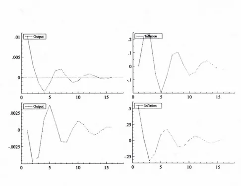
Figure 3: Impulse Responses V A R

Thus, above average output (inflation) tends to be followed by below average output (inflation) circa l| to 4 years down the road with the maximum effect after circa 2 - years .

Looking at the cross-correlations reveals that above average output is followed by above average inflation 0 to 10 quarters later, with the maximum correlation at 5 quarters. This suggests a considerable slack ness in the price response. Correspondingly, above average inflation is followed by below average output around 2 to 12 quarters later, with the maximum effect at around 6 to 7 quarters, making above average inflation a leading indicator o f below average output.

A n alternative way to look at the behavior of output and inflation is to consider the impulse response functions resulting from a statistical analysis of the data. The impulse responses depicted in figure 3 were

(14)

estimated by fitting a vector auto-regression (V A R ) with 2 lags to yearly data.5 Details of the estimation and the impulse responses for a V A R with 1 lag can be found in appendix 11.1.

The first row o f figure 3 shows the reaction of output and inflation to a one standard deviation output shock. Output remains about 0.3 standard deviations above average in the year following such a shock, illustrating that there is considerable output persistence. Inflation in creases by 0.4 standard deviations in the two years after such a shock, which demonstrates that the data exhibits a strong slackness in the price response.

The second row of figure 3 shows the reaction of the two variables to an inflation shock of one standard deviation. Inflation remains only slightly above average in the year after the shock suggesting that infla tion shocks have less persistent effects on inflation than output shocks. Output itself decreases by more than 0.4 standard deviations in the two years after the inflation shock. Inflation shocks are thus strong leading indicators of below average output.

From the analysis above one can conclude that output shocks cre ate a persistent output increase and an even more persistent inflation increase. Moreover, inflation is persistent and creates a persistent de crease of future output. Führer and Moore [11] have reported largely similar results for the autocorrelation functions of an estimated V A R on output, inflation, and the 3 months T-bill rate.

Although the presented facts nicely confirm conventional wisdom about the dynamic interaction of output and inflation in the economy, these facts contrast strongly with the ability of business cycle models to match them. Chari, Kehoe, and McGrattan [22], for example, illustrate the problem that standard sticky price models have in generating suffi cient persistence in these variables. Nelson [19] illustrates the difficulties 5 Yearly data was obtained by calculating averages of the quarterly values of each calendar year. Estimating yearly data improves the robustness with respect to the statistical specifications and facilitates the comparison with the theoretical section in the remaining part of the paper.

(15)

of a range o f models in replicating the observed persistence of inflation rates.

The important feature of the model presented in the remaining part o f this paper is that it can replicate all of the facts outlined above without recourse to appropriately specified exogenous shock processes or adjustment costs.

3 A Simple Business Cycle M odel

This section outlines a dynamic macroeconomic model with sticky prices where money is introduced through a cash-in-advance constraint. The reduced form o f the model can be summarized by three equations:

n £ = n twt] (

1

)

1 — O’

div dii)

= w (yu E t[Ut+l\) with ~ > 0 ,

— 7

> 0 (2)

y t - i . , / 0 \

Vt = + (3)

n t denotes the inflation factor, y t real output, Wt the real wage, and

g > 0 the level of real government expenditure. vt is a white noise (government) demand shock, <r is a parameter describing the degree of imperfect competition in the economy, and E t[-] denotes the expectations based on information up to time t.

Equation (1) describes the inflation factor resulting from the price setting behavior of profit-maximizing entrepreneurs who are in imper fect competition and who set their prices one period in advance. Such entrepreneurs mark-up over expected production costs, see Dixit and Stiglitz [7]. W ith a linear production technology that transforms labor into consumption goods and an appropriate normalization of labor, nom inal production costs are given by PtWt. The mark-up factor is given by y ^ , where a € [ 0 ,1[ denotes the inverse of the elasticity o f substitu tion between the goods of different entrepreneurs. Optimal price setting

(16)

behavior thus implies

Pt = Y ~ E t-\ [P tW t\

1 — CJ

Dividing this equation by the period t — 1 price level Pt~

1

delivers equation ( l ) . 6

Equation (2) describes the equilibrium real wage of the economy. The wage rate increases in the demand for labor and in the expected inflation tax. Labor supply functions that deliver these properties can be derived from workers who maximize the following lifetime objective

max s.t. ci m ] , < l~l -

nt

m\ m Ui

n,

cJ + n\wt (4) (5)

where c\ denotes consumption, n\ the labor supply, and m\ the real money holdings at the end of period t. Equation (4) is the cash-in-advance constraint that forces workers to use cash to pay for consumption goods and equation (5) is the budget constraint. W hen u, v £ C 2, v! > 0, u" <

0, u ffi'c > —1 for all c > 0, v' > 0, v" > 0, and when the cash-in- advance constraint is binding, utility maximization implies the following labor supply function:7

nt = n (wt, £ t[II{+i]) with > 0, — t < 0

dw t o E t\\\t+i\

6The fact that there is no supply shock present is not crucial for what follows. It is just a convenient assumption that simplifies the algebra. All results are continous to the introduction of a small supply shock.

7It is safe to assume here that the cash-in-advance constraint will be binding. Along an equilibrium path with positive inflation rates the constraint will bind whenever surprise inflation IIt+i — [IIt+i] is not too negative. Then agents do not end up with unexpectedly high real money holdings that they want to carry over into the next period. © The Author(s). European University Institute. produced by the EUI Library in 2020. Available Open Access on Cadmus, European University Institute Research Repository.

(17)

Inverting this labor supply function with respect to the first argument and imposing competitive market clearing delivers the equilibrium real wage of equation (2).

Equation (3) describes the demand side of the economy. Since prices are preset, output is determined by demand in the short run. W ith the cash-in-advance constraint binding, demand from the private sector (workers and entrepreneurs) is equal to the real value of their money holdings, which is given by The demand of the government is equal to g + vt, which is assumed to be financed through seignorage. This implies

yt = m t = — — + g + vt

lb and delivers (3).

From equations (1) to (3) one can obtain two equations describing current output and inflation in the economy as a function of past variables and expectations about future inflation:

— — ~Et_i[U tw(^—— h g + vt, IIt+i)] i — <T l l t Vt ( 1 - <r)yt-\ E t -i[IItu ;(J^ 1- + g + vt, IIt+i)] + g + vt

(6)

(7) The remaining part of the paper will consider limit economies with gov ernment expenditures gs > 0 where lim ^oo gs — 0. If some variable i , - t J a s s - > oo, I will write x s sa x.

4 Rational Expectations Equilibria

The stationary rational expectations equilibrium of interest for the de terministic version of the model is given by:8

IT « 1

y a « n ( l - <r, 1)

8The model can have a second stationary rational expectations equilibrium with the property that government seignorage is a large fraction of output. Since this contradicts U.S. data, consideration of this equilibrium will be deferred to section 9.

(18)

Equilibrium inflation is slightly positive but approaches zero as the level of government seignorage g approaches zero.9 Linearizing (6) and (7) around the deterministic steady state yields an approximation for the stochastic system: n £ Vt

+

- 1 2 y° 1 - y “

+

l -i

cn ,ui

- ! / * ( 1 - E T l ) Et_r [n £ E t- i [n t+1] + _IV'Cn.w ₁ Vt-i + vt (

8

)

where en u, denotes the elasticity of labor supply at the deterministic steady state.

In appendix 11.2 it is shown that all rational expectations solu tions to (8) have a minimum state variable representations as a two- dimensional A R (1 ) process n ( Vt — a -f B n £_ ! Vt-1 (9a)

Appendix 11.2 also shows that there is a stationary rational expectations solution given by

n t

Vt ( 10 )

Output in this equilibrium is white noise and inflation is lagging output deviations by one period. There exists also a non-stationary rational expectations solution given by:

(

n £ Vt n £_ i m - i ( i i )

9 Remember that n t = denotes the inflation factor and approaches one as inflation approaches zero.

(19)

where Wi denotes the derivative of w(-, •) with respect to the i-th argu ment, evaluated at the deterministic steady state. A s one can easily see, this equilibrium path is diverging from the steady state. Th e diverging paths have either increasing inflation rates and decreasing output levels or decreasing inflation rates and increasing output levels.10

5 Learning to Forecast Inflation Rates

This section introduces agents who do not possess rational expectations right away but who are learning in a similar way as real-life econometri cians.

Agents are endowed with a given set of statistical techniques which they apply to the data that is available up to date in order to make forecasts about the future evolution of the economy. A s more data be comes available, agents revise in real-time their models and parameter estimates. Thus, as the economy evolves agents learn about which econo metric model to fit to data and about the parameters of the models. Since their inferences inform their decisions, learning feeds back into the evolution of the economy.

To model learning about forecast models, agents are assumed to consider a given class of econometric models, the idea behind this being that the class o f forecast models is determined by agents’ econometric capabilities. By endowing agents with more or less econometric knowl edge one can generate more or less clever agents which consider larger or smaller classes o f forecast models.

A given endowment with econometric techniques can be interpreted in different ways. One interpretation is that agents possess a statistical software-package that offers some standard features that can be imple mented by pushing buttons but that they are unable (or find it too costly) l0The path with increasing output levels exists only in a local sense, see Adam [1] for details. © The Author(s). European University Institute. version produced by the EUI Library in 2020. Available Open Access on Cadmus, European University Institute Research Repository.

(20)

to expand the capabilities of the package. Alternatively, one could in terpret the class of models as the set of models that is covered by the current frontier of econometric knowledge.

For analytical reasons, agents in the present model are rather simple- minded econometricians. In particular, agents are assumed to be able to perform just ordinary least squares estimation of simple regression mod els of the form

I I t = Q + j + e t

where x is an explanatory variable. One should not take this assumption too literally but rather as a short-cut for more sophisticated agents in a more sophisticated environment. Moreover, as will become clear be low, such agents are sufficiently clever to potentially behave like rational forecasters in the limit.

W ith the economy being described by two state variables, real out put and inflation, the class of simple regression models that is associated with the above endowment of estimation techniques contains only two models:

Model 1 : n t = a 1 -I- fixyt

- 1

Model 2 : IIt = a 2 + /32Tlt^

Clearly, the class of forecast models is large enough to encompass the rational expectations equilibria of the economy: Model 1 generates the rational expectations of the stationary equilibrium (10) for a 1 = 0 and /?’ = and generates the rational expectations of the non-stationary equilibrium (11) for a 1 = 1 + ys and /31 = — jj£. Model 2, however, will never generate rational expectations. Yet, agents consider Model 2 because it is o f the same complexity as Model 1.

It remains to determine how agents choose between the different forecast models. There is a long and controversial debate in econometrics about how one should choose, construct, modify, and test econometric models in order to get the ’’ true” model. The purpose of this paper is not to add to this discussion. Instead I will simply assume that agents

(21)

choose the model with the lowest mean squared forecast error in the past. Agents, thus, do assign probabilities to different models according to the likelihood with which they believe them to be the right forecast models but rely entirely on the model with the best past performance (in the above sense).11

Using the mean squared forecast error as a selection criterion is identical to using the 7?2-value of the regression models as a selection criterion. Although choosing models according to .Revalues is somewhat ad-hoc, it can be defended on several grounds.

First, the R2-value is equal to the square of the correlation coeffi cient between the data and the fitted values. It is therefore a measure of the model’s predictive power over the sample period.12 W hen predic tive power in the past is an indicator for good prediction performance in the future then models with higher R2 should indeed be the preferred forecast models.

Second, the R2 measure is strictly increasing with the F-Statistic on the significance of all retained variable regressors.13 In this sense the model with the higher R evalue contains the more significant regression variable x.

Third, other more sophisticated selection criteria also face short comings such as the sensitivity of the results to the order of the tests that are applied to the statistical models.14

Given agents’ choice of forecast models and the point forecasts gen erated by the selected forecast model, each agent maximizes her payoff under the assumption that the future evolution of the economy is given

11 My conjecture is that none of the results would be altered when agents would as sign probabilities as long as updating of these probabilities is governed by the models’ performance in terms of their relative mean squared forecast errors.

12Note that this holds only for single equations regressions that assume uncorrelated errors and include an intercept term, see chapter 6.2 in Judge et. al. [12].

13c.f. the previous footnote.

14See also chapter 11 in Judge et al. [12] for a whole list of model selection criteria and their shortcomings.

(22)

by the point forecast. Such an approach is justified on the following grounds: Given the unbiasedness of least-squares based forecasts, the point forecast can be interpreted as the expected realization of the fore casted variable. Since I consider local convergence in a linearized version of the economy, certainty-equivalence holds.

6 Defining Equilibrium

Given the assumptions of the previous section, the economy now evolves as follows: Each period agents estimate Model 1 and 2 by ordinary least squares and choose the model with the lowest past mean squared forecast error to forecast inflation. Given the inflation forecasts, firms’ price set ting behavior and workers’ labor supply decisions result in new inflation rates and output levels according to equation (8), where the operator

E [•] might now denote the potentially non-rational expectations of the chosen forecast model. Given the new data point, agents adapt their least squares estimates and their model choices.

A n equilibrium is then a situation where the new inflation rate and output level confirm the previous least squares estimates and the previous choice of forecast model, formally:

D e fin itio n 1 An equilibrium with simple regressions consists o f least squares estimates ( a 1*, /31*) and (a 2*, /32*) fo r Model 1 and 2, respectively, and all agents using either Model 1 or Model 2 to forecast inflation rates such that

i. Agents choose the model with minimum mean squared forecast er ror.

ii. Given the forecast behavior, the economic outcomes resulting from (8) reconfirm the least squares estimates ( a 1* ,/? 1*) and ( a 2* ,/?2’ ).

A n equilibrium where agents use Model i (i = 1 ,2 ) to forecast inflation will be called a Model i Equilibrium.

(23)

Before moving on to determine the equilibria o f the economy, I discuss some implications of the previous definition.

Suppose agents use Model 1 to forecast inflation rates. The tempo rary equilibrium relation (8) then implies that the actual law of motion for inflation is given by

n t =

0

(

0

*, (31) + b(al, p 1)yt- i

and coincides with the structural assumption of Model 1. This in turn implies that in a Model 1 equilibrium it must be that o ( a \ bl ) = a 1 and

b(al,/31) = /31, since otherwise the parameter estimates would not con verge. A s a result, a Model 1 Equilibrium must be a rational expectations equilibrium.

A t the same time, not every rational expectations equilibrium of the form n ( = a + by

t- 1

is a Model 1 Equilibrium in the above sense. Point 2 of the equilibrium definition requires that the least squares esti mates get reconfirmed at such an equilibrium, implying that only rational expectations equilibria which are stable under least squares learning of the corresponding forecast model fulfill this requirement.

Next consider the case where agents use Model 2 to forecast infla tion rates. Substitution of Model 2 expectations into (8) reveals that the actual law of motion for inflation is given by

n t = c*(a 2, /32) + Cl( a 2, P2) n t- i + c2( a 2, p 2)y t^ (14) where Cj(q2,/9 2) / 0 and C

2

( a 2,/? 2) ^ 0 .15 Note that the actual law of motion for inflation does not coincide with the structural assumption of Model 2. Furthermore, the actual law of motion lies outside the class of models that agents consider. A s a result, all considered forecast models are necessarily misspecified in some way: W hile Model 1 does not condi tion on past inflation rates, Model 2 does not condition on past output. l5The first inequality holds almost sure for any parametrization o f the economy and any values of a 2 and 0 1.

(24)

Which of the two models gives a better fit to (14) then depends on the parameterization of the economy.

Note that agents could not estimate (14) by a least squares regres sion of n e = q + Pyt

- 1

+ 7 llt _ i. Since output and inflation are both endogenous variables, the regressors are not independent, which results in biased least squares estimates. To be able to estimate the actual law of motion (14) an agent would have to expand the class of forecast models to two-dimensional vector auto-regressions.

There is empirical evidence from inflation expectations surveys that support the observation that agents’ inflation forecasts do not make effi cient use of the information contained in all variables (Ball and Croushore [2], Batchelor and Dua [3]). Interestingly, Batchelor and Dua [3] report that agents make efficient use of the information contained in past infla tion rates but do not make efficient use of the information contained in the money stock, which is the case when agents use Model 2 to forecast inflation, see (14).

7 Equilibria with Simple Regressions

This section determines the equilibria with simple regressions. Their properties are then analyzed and compared with each other in the next section.

7.1 Model 1 Equilibria

Determining Model 1 equilibria is straightforward. Since Model 1 equi libria are rational expectations equilibria there are only two candidates, the stationary rational expectations solution (10) and the nonstationary rational expectations solution (11).

Appendix 11.3 shows that the coefficient estimates ( a 1,/? 1) diverge over time from the non-stationary rational expectations solution. As de mand shocks hit the economy, agents adapt their least squares estimates

(25)

( a 1,/? 1) in a way such that their new expectations lead to new inflation rates and output levels that cause these estimates to diverge even further. On the other hand, the appendix shows that these estimates return over time to their equilibrium values at the stationary rational expectations equilibrium .

The non-stationary rational expectations solution, therefore, does not fulfill requirement (2) of the equilibrium definition implying that the stationary rational expectations solution (10) is the unique Model 1 Equilibrium.

7.2 Model 2 Equilibria

To determine the Model 2 equilibria substitute the inflation expectations in (8) by the predictions of Model 2 with parameters (a , (3). This delivers an equation describing current inflation and output as a function of the past values of these variables, the parameters (a , (3), and the real wage elasticity of labor supply en u,:16

/ n t W -

1

+ « (

2

+ / ? - £ ) \

**\ y * J**

V

( 2 - a ( 2 + ( 3 - - ^ ) ) y )

Ilt -i

Vt-1

(15)

In a Model 2 equilibrium the least squares estimate (3 is identical to the correlation coefficient 1 ^ of process (15). A s shown in appendix 11.4, this implies that (3 solves

0 =

( l + Z J - ^ / l + l - ^ ' E n,tu ' c n .u

(16)

I6A11 relevant properties of this process are unaffected by the level of output y.

(26)

Figure 4: 0 as a function of en<w

The unique real solution to this equation is given by

0

= y z - l 3£n +

9 ( £ n,w ) \ [z 3 e ni, where

_ 1 2 —

9en,w ~

27 (en,w)

+ 27 (ffn,tu)

= 54“ “

(£»,w)3

+ t / ( - 5 + 26e» . - + 9 (£" . “ )2 - 54 (£" . - ) 3 + 27 (£" . - ) 4)

\Entw ) '

Substituting the solution for 0 into (15) and setting a = IT (1 — 0 ) yields a candidate process for a Model 2 equilibrium. The properties of this process depend only on the elasticity of labor supply en>w. Numerical calculations show that it is stationary for 0.35 < e„iU, < 2 .1 5 .17

Figure 4 depicts 0 as & function of the elasticity of labor supply and reveals that 0 is increasing in e n<w with 0 = 0 for en<w = 1. There

17The boundaries are only approximate.

(27)

Figure 5: Mean Squared Forecast Errors when Agents Use Model 2

exists a simple intuition underlying the shape of the graph: For e „ iW = 1 a 1% demand shock causes a 1% increase in expected labor costs. W ith firms setting prices by marking up over expected costs this leads to a 1% inflation increase. This amount of inflation just devaluates excess money back to its equilibrium level. A s a result, there is no persistence in excess demands, inflation is white noise, and /3 = n‘) ' s efl ua* to zero.

A s labor supply becomes more elastic, then a 1% demand shock leads to less than a 1% labor cost and inflation increase. The excess money stock is then not devaluated in a single period but persists to the next period where it results in a further inflation increase. A s a result, inflation rates are positively auto-correlated with the auto-correlation increasing in the elasticity of labor supply, hence the positive slope in figure 4.

An increase in

£n<w

not only increases the auto-correlation o f infla tion but also reduces the marginal impact o f past output on inflation,

(28)

which is given by ^-1—A, see equation (15). Thus, higher elasticities of labor supply should improve the performance of forecast Model 2 and worsen the performance of Model 1.

This intuition is confirmed in figure (5) which shows the mean squared forecast errors of Model 1 and 2 under the assumption that agents use Model 2 for forecasting. For £„jU, > 1.75 Model 2 performs better than Model 1.

Appendix 11.3 shows that the candidate process (15) is stable un der least squares learning of Model 2, regardless of the value of £n,w-

This establishes that Model 2 equilibria exist for labor supply elasticities between 1.75 and 2.15.

The required elasticity might seem high at first sight but such elas ticity levels are not uncommon in the literature. Christiano, Eichenbaum, and Evans [15], for example, find satisfactoiy performance of a limited participation model for similar levels. Moreover, high elasticities might mimic features, such as labor market frictions, which remain unmodeled in this paper (Jeanne [13]).

8 Equilibria with Simple Regressions and

the Business Cycle

This section studies the properties of Model 1 and Model 2 equilibria and compares them with the properties of U .S. data presented in section 2.

8.1 Output and Inflation in Model 1 Equilibrium

From (10) it follows that output and inflation in Model 1 equilibrium are given by rr vt-1 y“ + vt-1 Ut — — r — — *— y y yt = y s + vt © The Author(s). European University Institute. produced by the EUI Library in 2020. Available Open Access on Cadmus, European University Institute Research Repository.

(29)

\ --- V — ---

—

_—

: i ; : • • • • • |

—

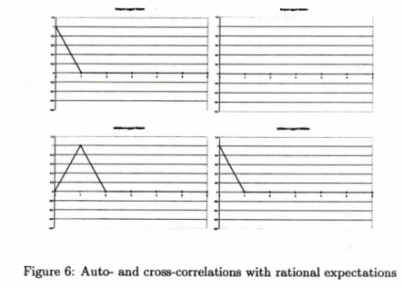
-Figure 6: Auto- and cross-correlations with rational expectations

Inflation and output are white noise but, due to sticky prices, inflation deviations lag output deviations by one period.

A government demand shock

vt

temporarily increases output and money holdings. The increased money stock (correctly) causes inflation expectations to increase by an amount that implies that the increased money stock will be devaluated by the next period. The increased in flation expectations then causes entrepreneurs to increase their prices by exactly an amount that makes these expectations become true, see (1). Shocks, therefore, show no persistence.

Figure 6 depicts the auto- and cross-correlations o f output and in flation in Model 1 Equilibrium. It performs rather weak when compared with figure 2 for U.S. data. The rational expectations equilibrium per forms reasonably well only along one dimension: current excess output leads to inflation in the subsequent period, which is due to the sticky price assumption. 23 © The Author(s). European University Institute. version produced by the EUI Library in 2020. Available Open Access on Cadmus, European University Institute Research Repository.

(30)

;

\ y

\ /

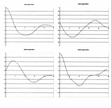
Figure 7: A u to - and cross-correlations in Model 2 Eq.

8.2 Output and Inflation in Model 2 Equilibrium

This section presents the properties o f Model 2 Equilibrium. Throughout the section it is assumed that the elasticity of labor supply is given by

£n,w — 1.8, which is at the lower end of the range for which Model 2 Equilibria exist. A low elasticity value has been chosen because higher ones would generate even more persistence, as is argued towards the end of this section.

Figure 7 depicts the auto- and cross correlations of output and inflation in Model 2 Equilibrium. The data is shown for 6 periods, which corresponds to 24 quarters of U.S. data if each model period is interpreted as 1 year. The shapes o f the auto- and cross-correlations correspond remarkably well with the correlation in the data. Output and inflation are persistent. They are positively correlated for short lags and negatively for longer lags. O utput is a positive leading indicator for inflation and, more importantly, inflation shocks are a leading indicator for decreasing

(31)

output.

A s in the data, the lag length at which correlation o f output with past output is zero roughly corresponds with the lag length at which the correlation o f inflation with prist inflation is zero. Furthermore, at this lag length the cross-correlations of output and inflation have their respective maximum and minimum.

To understand how the above result emerges consider agents’ esti mates of the two forecast models in Model 2 Equilibrium:

Model 1 : n t = (1 - 0.467) + _{y S}

1

Model 2 : n f = (1 - 0.688) + 0.688II£_i

The estimate of the AR-coefficient of Model 1 shows that inflation in a Model 2 equilibrium is reacting much weaker to an output deviation than in Model 1 Equilibrium where the same coefficient is given by -V, see (10).

This relatively weak reaction o f inflation to a demand shock is due to an elastic labor supply and the use of Model 2 as a forecast model. Re member the equation describing firms’ price setting behavior, reproduced here for convenience:

P i

= L — O’

In the period after a demand shock, firms increase their prices because they expect wages to increase.18 However, since they condition their inflation expectations on past inflation and not on past output, their in flation expectations do not pick up in response to a demand shock. W ith an elastic labor supply, costs increase only slightly and prices therefore respond sluggishly.

A s a result the demand shock persists into the second period after the shock and causes wages again to be above equilibrium. Since inflation

18In the period of the shock prices are already set and cannot react. 25 © The Author(s). European University Institute. version produced by the EUI Library in 2020. Available Open Access on Cadmus, European University Institute Research Repository.

(32)

•" X

\

,_N

/

\

/

\

/

X

\ • • • / • • ’ • \ •

- ■

"

^

-J

\

/

V /

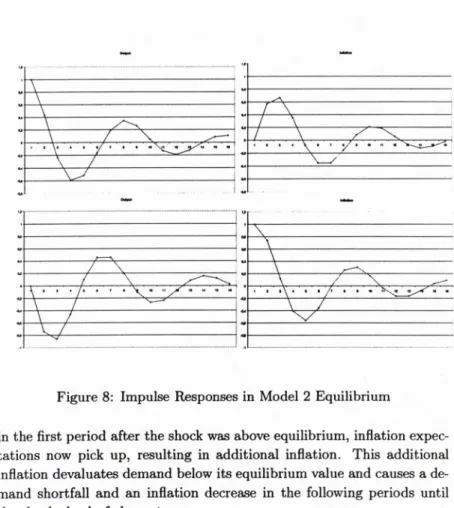
Figure 8: Impulse Responses in Model 2 Equilibrium

in the first period after the shock was above equilibrium, inflation expec tations now pick up, resulting in additional inflation. This additional inflation devaluates demand below its equilibrium value and causes a de mand shortfall and an inflation decrease in the following periods until the shock slowly fades out.

The first row of figure 8 shows the impulse responses of output and inflation that follow a demand shock that hits the economy in period 1. The impulse responses graphically illustrate the mechanism described above: the initially sluggish price response in period 2 causes output to remain above equilibrium in the period after the shock. W hen inflation expectations pick up in period 3, inflation is so high that it causes a demand slump in the subsequent periods, and a corresponding drop in

(33)

inflation. The effects then slowly fade out. For completeness, the second row of figure 8 shows the impulse responses to a (non-modeled) inflation shock. Th e intuition for their shapes is analogous to the one above.

Note that the impulse responses of figure 8 nicely match the esti mated impulse responses for U .S. data shown in figure 3.

The impulse responses reveal that output in Model 2 Equilibrium displays a higher variance than in Model 1 Equilibrium for the same sequence of underlying shocks vt : In Model 2 Equilibrium demand shocks create output variations even a long time after their occurrence. A t the same time, the initial output reaction to a demand shock is the same in both equilibria.

W hether inflation in Model 2 Equilibrium is more volatile as well is unclear because inflation initially reacts less to an output shock when compared to its reaction in Model 1 Equilibrium. However, simulations showed that, at least for en<w = 1.8, inflation is also more volatile in Model 2 Equilibrium.

For higher values of the elasticity of labor supply, the impulse re sponses and the persistence of output and inflation deviations become even stronger than shown in the figures above. Demand shocks then lead to an even more sluggish response in costs and prices, which generates increased persistence. For lower values, e.g. for en,w — 1-75, the results are almost indistinguishable from the ones presented above.

9 M odel Choice and ’U nstable’ Rational

Expectations Equilibria

In the previous sections it has been shown that agents might prefer to use forecast models that generate inefficient forecasts. The purpose of this section is to show that this can cause the economy to be close to a rational expectations equilibrium that is unstable under learning of consistent forecast models.

27 © The Author(s). European University Institute. version produced by the EUI Library in 2020. Available Open Access on Cadmus, European University Institute Research Repository.

(34)

This point is of interest because the instability of a particular ratio nal expectations equilibria under adaptive learning of consistent models has typically been interpreted as such equilibria being unlikely economic outcomes, e.g. Evans and Honkapohja [10]. This section shows that such ’unstable’ equilibria can nevertheless give (in average terms) good predictions o f the economic outcomes.

I first construct a rational expectations equilibrium that is unstable under least squares learning of consistent forecast models.

To this purpose assume that there exists an inflation tax n max < oo above which agents decide not to supply any labor when the wage is given by w = 1 — a.19 This implies that the deterministic version of the model possesses a second stationary rational expectations equilibrium where output y ss is close to zero and inflation II** is close to IImax.20

After linearizing (6) and (7) around this steady state one finds two rational expectations solutions. Again, there is a stationary solution and a non-stationary solution with inflation following lit = and n t = n ss — respectively. Note that Model 1 is a consistent model for these rational expectations equilibria. It is easy to show that both rational expectations solutions are unstable under least squares learning of Model 1.

Nevertheless, there exist Model 2 equilibria that are close to the high inflation rational expectations equilibrium. To show existence of such equilibria, assume that the labor supply function is given by21

_ i £ t[nt+1]

'H

OL W t

19A sufficient condition for this is tt'(0) < oo.

20The details of this and the following arguments can be found in Adam [1]. 21 Such a labor supply function can be derived from agents that maximize the fol lowing lifetime objective:

max Eq OO ^ 2 log(l + Ct) - an, ,t=o subject to Ct < 1 and m , = — Ct + ntwt . © The Author(s). European University Institute. produced by the EUI Library in 2020. Available Open Access on Cadmus, European University Institute Research Repository.

(35)

0 0.025 0.06 0.075 0.1 0.125 0.15 0,175 0.2 0.225 sigma

Figure 9: Model 2 Equilibria at the High Inflation Steady State

The model is then described by two parameters, the marginal disutility of labor a and the degree of imperfect competition a.

Using computational methods, a grid search was made to check for the existence of Model 2 equilibria across the relevant (a , a)-space.22,23 The shaded area in figure 9 indicates some part of the parameter space for which Model 2 Equilibria exist.22 23 24 Although the area is rather small, the graph reveals that it has positive mass.

22The other parameters were set to g = 0.02 and vt ~ U [—0.005, +0.005].

23Let agents estimate and use Model 2 to forecast inflation. Calculate new inflation rates and output levels according to the linearized version of (6) and (7). Agents update their estimates until they have converged to some value (a, 0 ). The converged values are a potential candidate for a Model 2 equilibrium. Simulate the economy with Model 2 and (a, 0 ) and calculate the mean squared forecast errors. Fit Model 1 to the simulated data and calculate the forecast errors. If these are higher than with Model 2, a Model 2 equilibrium has been found.

24Model 2 Equilibria exist also for a > 0.225 and a < 0.61. 29 © The Author(s). European University Institute. version produced by the EUI Library in 2020. Available Open Access on Cadmus, European University Institute Research Repository.

(36)

Noting that average output and inflation in the Model 2 Equilib rium is equal to average output and inflation in the rational expectations equilibrium, the example shows that an economy with learning agents can be close to a rational expectations equilibrium that is unstable un der learning of consistent forecast models.

10 Conclusions

Agents that consider a class of forecast models might well choose to use a model that is inconsistent with rational expectations, even though the considered class contains forecast models that are consistent with rational expectations. This can happen whenever use of a particular forecast models from the class leads to an actual law of motion of the economy that lies outside the considered class of models.

W ith inconsistent forecast models agents’ equilibrium expectations are inefficient, as suggested by inflation expectations surveys. Moreover, equilibria with inefficient expectations are able to reproduce important features of the data such as the shape of the auto- and cross-correlations of output and inflation and the impulse response functions for demand and supply shocks.

Some implications and questions raised by these findings might de serve further attention.

Firstly, one could construct models with agents that consider dif ferent classes of forecast models. This is likely to produce heterogenity of forecast models and actual forecasts. It will be interesting to check whether heterogeneity along these lines makes it even more difficult for forecasters to detect the true underlying economic relationships.

Secondly, since Model 2 Equilibria are Pareto dominated, one might ask whether policy makers could influence the use of forecast models, e.g. through an appropriate monetary policy, and move the economy from a Model 2 Equilibrium to the rational expectations equilibrium.

I hope to provide answers to these questions in future contributions.

(37)

1 1

A ppendix

11.1 Vector Auto-Regression

A V A R with two lags and a constant was estimated by O LS regression. The data consists of the of the bandpass-filtered quarterly inflation and output data depicted in figure 1. The estimation results are :

lit Std.E rror yt S td .E rror const. 0.020562 0.089495 0.00033680 0.0016824 n t_ i 0.056692 0.16023 -0.0087039 0.0030122 lit—2 -0.39029 0.15483 -0.0042423 0.0029107 2/t-i 22.005 8.7542 0.29932 0.16457 Vt-2 15.306 9.2518 -0.035335 0.17393 a 0.55062 - 0.010351 -R2 0.75406 - 0.69924

-The actual and the fitted values are shown in figure 10. Figure 11 depicts the auto-correlation of the regression errors. If one required regressors to be significant at the 1% level, one could test down to a model with just 1 lag. Figure 12 shows the impulse response functions for this case and illustrates the robustness of the impulse responses.

11.2 Calculation o f the Rational Expectations Equi

libria

Linearization of (6) and (7) around the steady state and noting that

a%!iL 7 = 1 — <7 and ^ • l 3^ = —— at the steady state delivers (8). Applying the techniques of proposition 1 in Evans [8] one can prove the following lemma:

L e m m a 1 Consider a stochastic linear expectational difference equation o f the form,

Xt — k + B oE t-i [it] + [it+i] + D x t- i + Ut (18)

3 1 © The Author(s). European University Institute. version produced by the EUI Library in 2020. Available Open Access on Cadmus, European University Institute Research Repository.

(38)

Figure 10: V A R : Actual and fitted values

O

I

2

3 4 5

Figure 11: V A R : Autocorrelation of residuals