Generation and manipulation of multiphoton quantum fields

(1)

Universit´a degli Studi di Roma Tre

e

Consorzio Nazionale Interuniversitario per le

Scienze Fisiche della Materia

Dottorato di Ricerca in Scienze Fisiche della Materia

XXIII ciclo

Generation and manipulation of multiphoton quantum fields Tesi di dottorato della dott. Chiara Vitelli

Relatori: Coordinatore Dottorato:

Prof. Francesco De Martini Prof. Settimio Mobilio

Dr. Fabio Sciarrino

(2)

(3)

Introduction

In the context of modern science, Quantum Information opens a new chapter, whose ori-gins can be traced down to a proposal by Richard Feynman in the early eighties of the last century [Fey82]. According to Feynman aquantum computer, i.e. a device working on the basis of the algorithms of information theory re-formulated within the Hilbert space sce-nario, would be a necessary tool to simulate and investigate properly any natural quantum process. Owing to its insightful predictive character and to its intrinsic multidisciplinary nature, Quantum Information has attracted scientists from diverse areas of theoretical and experimental physics, e.g. atomic physics, quantum optics and laser physics, condensed matter, etc., and from other disciplines such as computer science, mathematical complex-ity, material sciences and engineering. In the last two decades it has undergone a huge and rapid growing, both on the theoretical and experimental sides and, in a world moving fast towards an increasing miniaturization approaching the quantum limits, it is expected to revolutionize many areas of Science and Technology. Today one of the main goals of QI is to understand the subtle aspects of quantum mechanics in order to learn how to formulate, manipulate, process and communicate the information in the most efficient way using realizable physical systems that operate on quantum principles. This is quite a hard task which necessarily implies a nearly decoherence-free intersection between the

microscopicworld of single quantum particles (photons, atoms etc.) and themacroscopic

preparing or measuring devices that transfer the information to the human world.

QI usually deals with quantum bits, or qubits, i.e. 2-dimensional quantum systems that generally do not possess the definite values of 0 or 1 of classical bits, but rather are in a so-calledcoherent superposition,|ψ⟩ =α|0⟩ +β|1⟩ of the two orthogonal basis states

{|0⟩,|1⟩}. Such state reveals unusual properties, especially when dealing with composite

systems. Indeed the most distinctive feature of quantum physics is given by the possibility of entangling different qubits. First recognized by Erwin Schroedinger as “the character-istic trait of quantum mechanics”, quantum entanglement represents the key resource for modern QI processing. It derives from subtle non-local correlations between the parts of a quantum system and combines three basic structural elements of quantum theory, i.e. the superposition principle, the quantum non-separability property and the exponential scaling of the state space with the number of partitions. Quantum entanglement has no classical analogue. This resource, associated with non-classical correlations among sep-arated quantum systems, can be used to perform computational and cryptographic tasks

(8)

8 INTRODUCTION

that are impossible with classical systems. An entangled state shared by two or more sep-arated parties is a valuable resource for fundamental quantum communication protocols, such as quantum cryptography and quantum teleportation. While quantum communica-tion tasks can be suitably realized with ”flying” photonic qubits, there are at present a number of technologies under investigation for their suitability to implement a quantum computer. No single technology meets currently all of these requirements in a completely satisfactory way. Indeed, besides photons, qubits can be in principle realized by using different resources, for instance trapped ions, neutral atoms in interaction with optical cavities, superconducting circuits, semiconductor quantum dots, impurity in solids and also by the nuclear magnetic resonance.

Quantum optics represents an excellent experimental test bench for various novel con-cepts introduced within the framework of QI theory. Indeed, quantum states of photons can be easily and accurately manipulated using linear and non-linear (NL) optical devices and can be efficiently measured by efficient single-photon detectors. Pairs of entangled photonic qubits are usually generated by the spontaneous parametric down conversion

(SPDC) process in a NL crystal where, under suitable conditions a pump photon of fre-quencyωpis annihilated and two photons of frequenciesω1andω2are created, such that

ω1+ω2=ωp.

Nevertheless, as said the main problem of quantum resources resides on the extremely fragile nature of quantum systems and on the decoherence process that affects the quan-tum world. A possible approach in order to overcome this limitation is to exploit an amplification process performed over the photonic qubit establishing a tight connection between the microscopic and the macroscopic fields. Such an approach is at the heart of this work, whose starting point is the possibility of generating multiphoton quantum states through non linear optical methods. The generated fields have been obtained through the interaction of a non linear crystal with a high power pump beam, by amplification of sin-gle photon states or by spontaneous emission in a high gain regime. The interest for the study of multiphoton fields generated by the optical parametric amplifier is double: on one hand there is the investigation about the nature of quantum mechanics and about the transition from the microscopic to the macroscopic world, i.e. from the quantum to the classical world. The study and the realization of the entanglement between macroscopic quantum fields, generated by high gain spontaneous parametric amplifiers, fits in with this context. On the other hand there is the practical interest of the quantum information field for the possibility of generating macro-qubits, resilient to decoherence and to losses, able to be used in different quantum information and quantum communication protocols. A further application of these states is related to the possibility of performing measure-ments able to influence the following overall state system evolution. Concerning this property, we have developed the idea of exploiting the high resilience to losses of the macro-qubit states in order to beat the decoherence in quantum metrology applications. Furthermore, in the quantum metrology context, the employ of this multiphoton states into interferometric schemes has been studied. More specifically the amplification of

(9)

INTRODUCTION 9

NOON states has been investigated, theoretically and experimentally, [VSSD09]; these states enable to increase the optical resolution in interferometric experiments, beating the Heisenberg limit, and resulting as a resource in the context of quantum lithography. Finally the interaction between multiphoton fields with atomic systems such as a Bose Einstein condensate (BEC) [DSVC10], by realizing the merging between different tech-nologies, could open a new scenario in the context of quantum information. For example the creation of the light-matter entanglement would represent a long term perspective for this application. The simultaneous adoption of different methods and concepts, i.e. the optical phenomena and the BEC, would led to the development of an hybrid technology

for the quantum information. The hybrid system would consist in the use of the two sub-systems , the optical and the atomic ones, that can be prepared, manipulated and measured through different and independent experimental technologies.

The present work is divided into four parts: in the first part the necessary elements of quantum information and quantum optics are presented: in chapter 1 the quantum state representation and the more important features of quantum states are addressed, while in chapter 2 the optical implementation of quantum states is investigated. Particular atten-tion is devoted to the concept of quantum cloning which is at the heart of the realizaatten-tion of multiphoton states of light. In part two two fundamental schemes for the macro states generation are then introduced: the quantum injected optical parametric amplifier (chap-ter 3), and the high gain optical parametric amplifier working in a spontaneous regime (chapter4). In both cases the quantum properties and the measurement strategy suitable for the observation of quantum nature are investigated. In this context the problem of find-ing a measurement able to catch the quantum structure of macro states arises. Hence in part three, by making use of optical devices such as an experimentally developed ultrafast optical shutter (chapter 5), we exploit different manipulation strategy in order to obtain the maximum amount of information about the multiphoton fields (chapter 6). Finally different applications of macro-states are investigated in part four: the high flux regime combined with the sub Rayleigh resolution available with an optical parametric amplifier working in a spontaneous emission regime turns out to be a promising ingredient to per-form efficient lithography experiments (chapter 7). In the quantum metrology context the robustness of macro states obtained by the amplification of single qubits has then been ex-ploited for improving the sensitivity in interferometrical experiments performed in high losses conditions (chapter 8. The same robustness allows in principle the non resonant interaction between the multiphoton state and a BEC system, theoretically investigated in chapter 9.

(10)

(11)

Part I

Preliminary notions

(12)

(13)

13

Figure 1: Conceptual scheme of the present work: the possibility of generating macro-scopic states of light is at the basis of the thesis. The multiphoton states can be generated through different amplification schemes. In both cases the measurement problem is a key ingredient for the observation of quantum properties. The macro-states can then be stud-ied as a paradigmatic example for the quantum to classical transition investigation. On the other hand the interest in investigating macroscopic states of light concerns the imple-mentation of quantum information protocols related to quantum metrology and light atom efficient interactions.

The framework of the present thesis is reported in figure 2.8. The starting point of this research work is the generation of multiphoton quantum states, through different optical systems based on the laws of quantum mechanics and realized with the tools of non linear optics.

In this part the preliminary notions about the basic concepts of quantum information and quantum optics are then given. The problem of representation of quantum states and their measurement, which is strictly connected with the possibility of observing quantum phenomena in an increasing size quantum system, is firstly approached. The concept of quantum cloning and its implementation through the optical parametric amplifier, which is at the basis of the experiments addressed in the next chapters, is investigated in connection with the quantum correlation measurements problem.

(14)

(15)

Chapter 1 Elements of Quantum Information

Quantum information is a generalization of classical information, a deep difference among the two is shown by Bell’s work (1964) [Bel64], in which is demonstrated that quantum reality cannot be reproduced by a local hidden variables model.

Quantum Information is then a non trivial extension of classical information which presents some limitation due to the laws of quantum mechanics: for instance two non commutative observables cannot be measured simultaneously, the acquisition of information about the system perturbs the system itself. This problem is strictly related with another difference between quantum and classical information: quantum information cannot be cloned (no-cloning theorem, demonstrated by Wooters and Zurek in 1982 [WZ82]).

The different resources and the “unusual” properties of quantum mechanics, for instance the concept of entanglement and the parallelism with which different logical functions can evolve, make quantum computation a precious instrument when the requirement is to solve complex problems. Complex ornot complex in the information language refer to the time needed to solve a given problem: there is a distinction between algorithms which can be solved in apolynomial time or in aexponential time. To an algorithm A it can be associated acomplexity function TA(N), where N is the input length calculated in

bits. TA(N) is then the maximum time required to solve the algorithm A. If, for instance,

algorithm A is the factorization algorithm, the required time for aquantum implementa-tion (Shor algorithm) is polynomial. This problem is instead unsolvable by a classical

implementation, and the problem is said to have a “NP complexity”.

In this chapter the resources of quantum information will be addressed: starting from the

quantum bit to the concept of entanglement, we will address the problem of representa-tion and measurement of quantum states. Finally the problem ofquantum cloningwill be introduced.

1.1 Quantum states and their representation

The Quantum information carrier, thequbit, is defined into a bidimensional Hilbert space

{|0⟩,|1⟩}, and then, differently respect to the classicalbit, which can assume only 0 or 1 15

(16)

16 Elements of Quantum Information

values, a general quantum state can be defined as:

|ψ⟩ =α|0⟩ +β|1⟩ (1.1)

withα andβ complex numbers, such that|α|2+|β|2= 1. Thanks to the superposition principle, a qubit can then be codified in an infinite number of states, while the classical bit lives in a bidimensional space.

A projective measurement of the state |ψ⟩ upon the basis {|0⟩,|1⟩} will give as a re-sult |0⟩ with probability |α|2 and |1⟩ with probability |β|2. Classically a probabilistic bit measurement can give 0 or 1 values with a probability p0 and p1 respectively, such

that p0+ p1= 1. The two measurement processes are not equivalent: the first difference

resides into the perturbative character of a measurement in quantum mechanics, whose action modifies the state. The second difference is given by the continuous parametersα andβ, which not only define the probability of a given result but define also a vector into the tridimensional space of spins. We can indeed consider the qubit as a 1₂ spin state, the parametersα andβ determine then the polar and the azimuthal anglesθ andϕ.

The evolution of a quantum state is reversible and is given by the Schr¨odinger equation:

H|ψ⟩ = i¯h∂|ψ⟩

∂t (1.2)

where |ψ⟩ can be a single qubit or a complex system composed by several interacting degrees of freedom, and H is the system hamiltonian. At a fixed time t the state vector of the system can be written as:

|ψ(t)⟩ = U|ψ(0)⟩ (1.3)

where U = exp[−i_¯h∫₀tdt′H]is an unitary operator.

The qubit evolution can then be found by applying unitary operators to the state vector

|ψ⟩, corresponding to different continuous symmetries acting on the physical system.

For each continuous symmetry R acting on the system there is a corresponding unitary operator U(R) commuting with the system hamiltonian H. Generally:

U(R) = eiθQ (1.4)

where Q is the symmetry generator.

A particular symmetry class is the one of rotations: given the angular momentum J = (J1, J2, J3), a rotation around the axis n of an angle θ, is represented by the following

operator [Sak94]:

R(n,θ) = eiθn·J (1.5)

The rotation generator is then the angular momentum operator. The rotations group has an irreducible bidimensional representation:

(17)

Quantum states and their representation 17 Jk= 1 2σk (1.6) where: σ1= ( 0 1 1 0 ) , σ2= ( 0 −i i 0 ) , σ3= ( 1 1 0 −1 )

are the Pauli matrices, which with the unitary matrix form a complete basis for the 2× 2 matrices. A generic 2× 2 matrix can then be written as:

U(n,θ) = eiθ2n·σ _{= 1 cos}θ

2 − in ·σsin

θ

2 (1.7)

In conclusion the qubit is a 1/2 spin state and a unitary rotation acting upon it is equivalent to a rotation of the spin itself.

A measurement on the qubit results in an irreversible change of the system’s state and it will always give a result equal to 0 or 1, corresponding to the projection of the qubit into the state |0⟩ or |1⟩. It is impossible to know the state of a qubit through a single measurement, nor if, before the projection, it was in a pure state or in a superposition of states. It turns out that the infinite amount of information contained into a qubit is reduced, at the measurement stage, to the one carried by a classical bit.

1.1.1 Density matrix

Let us consider a large number of non interacting quantum states, in which each element of the ensemble can be described by the state|ψ⟩. The overall ensemble is then described by thedensity operator:

ρ=|ψ⟩⟨ψ| (1.8)

which in the notation of states vector (1.1), can be written as:

ρ= ( α β )( α∗ _β∗ )₌( |α|2 αβ∗ βα∗ _|_β_|2 ) (1.9) The density matrix is connected with the information content, and then with the system entropy S by the relation:

S =−kTr(ρlnρ) (1.10)

where k is the Boltzmann constant. A pure ensemble, in which each member of the ensem-ble is in the same state, the entropy is zero, this means that there is no lack of knowledge about the state of the system.

(18)

∂ρ ∂t =

−i

¯h [H,ρ] (1.11)

from whichρ(t) = Uρ(0)U†. The unitary evolution of the density operator preserves the system’s entropy ∂S_∂t = 0.

The density matrix allows to describe the properties of a complex system, which is not representable by a single qubit. If we have a two-qubit system, being A and B the two subsystems; for instance in the state:

|ψ⟩AB=α|0⟩A|0⟩B+β|1⟩A|1⟩B (1.12)

a measurement on the state A corresponds to the application of the operator (MA⊗ 1B) to

|ψ⟩AB. The expectation value of such an observable is:

AB⟨ψ|(MA⊗ 1B)|ψ⟩AB=|α|2A⟨0|MA|0⟩A+|β|2A⟨1|MA|1⟩A (1.13)

which can be written as:

⟨MA⟩ = tr(ρAMA) (1.14)

whereρA=|α|2|0⟩A⟨0| + |β|2|1⟩A⟨1|reduced density matrix of the qubit A.

Since the expectation value of every observable M acting upon the subsystem can be written as:⟨M⟩ = tr(Mρ) =∑_apa⟨ψa|M|ψa⟩, the density operatorρArepresents the

en-semble of the all possible quantum states in which the subsystem can be with probability

pa.

Generally for a bipartite systemHA⊗HB, if{|i⟩_A} is an orthonormal basis for the system

A and{|µ⟩_B} is an orthonormal basis for the system B, an arbitrary pure state HA⊗ HB

is written as:

|ψ⟩AB=

∑

i,µ

ai,µ|i⟩_A⊗ |µ⟩_B (1.15)

where ∑_i,_µai,µ = 1. The reduced density matrix of the system A, is then obtained by

tracing over B the total density matrix AB, and is:

ρA = trB(|ψ⟩_AB⟨ψ|)

=

∑

i, j,µ

ai, ja∗j,µ|i⟩A⟨ j| (1.16)

which has the following properties:

• ρAis selfadjoint:ρA=ρA†

• ρAis positive: for each|ψ⟩A A⟨ψ|ρ|ψ⟩A=∑µ∑iai,µ A⟨ψ| i⟩A

2

(19)

Quantum states and their representation 19

• tr(ρA) = 1

Generally the density matrix state can bepureormixed, in the first caseρ_A=|ψ⟩_A⟨ψ| is a projector which acts on the unidimesional space of the vector |ψ⟩_A for which holds

ρ2₌_ρ_{; in the second case the density matrix is given by the sum:} _ρ

A=∑apa|ψ⟩A⟨ψ|

where 0 < pa< 1 and∑apa= 1. In the last caseρis given by the incoherent superposition

of states and the relative phases between the various|ψ⟩_Aare experimentally inaccessible.

1.1.2 Bloch sphere

Let us consider the case in which the system A is a single qubit, a graphical represen-tation of the density matrix can then be given by the Bloch sphere. In a 2× 2 Hilbert space a generic self-adjoint operator has 4 parameters and can be expressed in the basis

{1,σ1,σ2,σ3}. The density matrixρ can be written as:

ρ(P) =1 2 ( 1 +−→P · −→σ ) (1.17) where det(ρ) =1₄(1−−→P2). In order to have det(ρ)≥ 0 it is necessary that −→P2≤ 1; there

is then a correspondence 1−1 between all the possible matrices of the single qubit and the points of the tridimensional space 0≤ |−→P| ≤ 1. This sphere is usually calledBloch sphere.

Figure 1.1: Bloch sphere: there is a 1− 1 correspondence between the points of the sphere and the single qubit’s density matrix. The length of vector P defines the purity of the state, the states on the surface are pure while the mixed ones are internal vectors.

The states with|−→P| = 1 on the surface correspond to the states whose density matrix

has determinant equal to zero, and, since tr(ρ) = 1, the density matrix must have eigen-values 0 and 1. This means that the operators corresponding to the points on the surface are unidimensional projectors over pure states.

(20)

The state of the single qubit |ψ(θ,ϕ)⟩ can be seen as a 1₂ spin vector on the direction identified by the angles −→r and (θ,ϕ):

|ψ(θ,ϕ)⟩ = ( e−iϕ/2cos(θ₂) eiϕ/2sin(θ₂) ) (1.18) the density matix can then be written as:

ρ(r) =1

2(1 + −

→_r _{· −}→_σ₎ _(1.19)

where the length of r determines the purity of the state.

The qubit state can be implemented via a two level system, such as the photon’s polariza-tion [DS05], the state 1.1 can then be written as:

|ψ⟩ =α|H⟩ +β|V⟩ (1.20)

where|H⟩ and |V⟩ are the horizontal and vertical polarizations and can be represented by the column vectors

( 1 0 ) e ( 0 1 ) .

In this case the three axis of the Bloch sphere represent the linear polarizations (−π→H, −π→V),

linear at 45◦degrees 45◦(−π→+, −π→−), and circular polarization (−π→R, −→πL).

1.2 Measurement and evolution of quantum states

Let us imagine, we have with equal probability some 1₂ spin particles in one of the two non-orthogonal states|ψ1⟩ and |ψ2⟩, such that:

|⟨ψ1|ψ2⟩| ≡ cosα ̸= 0 (1.21)

These non orthogonal states cannot be identified with certainty, by performing a standard or von Neumann measurement,the best we can do is indeed to project the particle state in one of the two orthogonal states|ϕ1⟩ or |ϕ2⟩, chosen as near as possible to the original

states (see figure 1.2).

Figure 1.2: The identification of the two non orthogonal states|ψ1⟩ and |ψ2⟩

through a standard quantum measure-ment.

(21)

Measurement and evolution of quantum states 21

The measurement result will give |ϕ1⟩ or |ϕ2⟩, which will identify |ψ1⟩ or |ψ2⟩

respec-tively [HMG+96]. This process has an error probability:

q≡ Prob(err) = |⟨ψ1|ϕ2⟩|2=|⟨ψ2|ϕ1⟩|2=

1

2(1− sinα) (1.22) In some cases this strategy can be the non optimal one: instead of having a binary answer

|ψ1⟩ or |ψ2⟩ with a given error probability, we can add a third option: the inconclusive

result. After the test the state of the particle will determined as|ψ1⟩ or |ψ2⟩, or unknown

. A way to implement this test is to choose in a casual way, adding an auxiliary system, to project the particle’s state over the orthogonal space to |ψ1⟩ or to |ψ2⟩. If the state

is projected on the space orthogonal to |ψ1⟩ and the measurement’s result is positive,

we know with certainty that the initial state couldn’t be |ψ1⟩ and it was |ψ2⟩. On the

other hand if we obtain a negative result no deterministic conclusion can be reached: the particle could be in both the states. In this case the measurement is inconclusive and the result must be discarded. This kind of test is an example of generalized measurement, or POVM (Positive-Operator-Valued Measurement).

1.2.1 Orthogonal measurements

Each measurable physical quantityA is represented by an hermitian operator A into the Hilbert spaceH , and is known as an observable.

The principal property of an observable is that it has a continuous and complete set of eigenvalues, furthermore two eigenvectors corresponding to different eigenvalues result to be orthogonal. In a n-dimensional Hilbert space it is possible to write the completeness condition as:

n

∑

i=1

Pi= 1 (1.23)

where Piis the projection operator on the eigenvector|ϕi⟩.

A measurement of the physical quantityA can only give as a result one of the eigenvalues of A, and the state|ψ⟩ is projected on the corresponding eigenvector. This measurement is known as astandard ororthogonal measurement. The probability of obtaining the result

i is given by the superposition of the corresponding eigenvector:

p(i) =|⟨ϕi|ψ⟩|2 (1.24)

More in general, if the initial state is described by the density matrixρ, the probability of obtaining the result i becomes:

(22)

1.2.2 Generalized measurements

A generalized measurement corresponds to couple the system under investigation to an auxiliary one, the ancilla, and then perform a standard measurement on the overall system. A generalized measurement can be mathematically described through a set of positive non-commutative operators Qi, which satisfy the condition:

m

∑

i

Qi= 1 (1.26)

where m can be greater than the Hilbet space dimensionality of the system under exami-nation. Since the operators Qiare non orthogonal projection operators, this measurement

is known as non-orthogonal measurement. In the case of the discrimination between the states|ψ1⟩ and |ψ2⟩, even in a bidimensional space, we need a measurement which gives

three results: the|ψ1⟩, the state |ψ2⟩, or the inconclusive one. The probability of obtaining

a result i is :

p(i) = Tr(ρQi). (1.27)

withρdensity matrix of the initial state.

1.2.3 Geometric representation

The bidimensional space identified by the vectors |ψ1⟩ and |ψ2⟩ can placed into a

tridi-mensional space, whose third dimension is given by the state|ϕ0⟩, orthogonal to the initial

states (figure 1.3).

Figure 1.3: Identification of twonon-orthogonal states |ψ1⟩ and |ψ2⟩ through

a generalized quantum measurement.

We can imagine the unitary evolution U of the system in a three dimensional space as a three-dimensional rotation around the vector u1= √1₂(|ϕ1⟩ − |ϕ2⟩) of an angle θ. The

(23)

U|ψ2⟩ = 1 √ 2 ( −sinα 2 + cos α 2cosθ ) |ϕ1⟩+ 1 √ 2 ( sinα 2 + cos α 2 cosθ ) |ϕ2⟩+cosα 2 sinθ|ϕ0⟩ (1.29) Defining the roation angleθ such that cosθ = tanα₂, we obtain:

U|ψ1⟩ = √ 2 sinα 2|ϕ1⟩ + √ cosα|ϕ0⟩ (1.30) U|ψ2⟩ = √ 2 sinα 2|ϕ2⟩ + √ cosα|ϕ0⟩ (1.31)

Since now |ϕ0⟩, |ϕ1⟩ and |ϕ2⟩ are orthogonal, it is possible to separate them with an

or-thogonal measurement. The probability of obtaining an inconclusive result is then:

p(inconclusive result) = cosα. (1.32) In such a way the state can be identified with certainty at the cost of discard part of the data corresponding to the inconclusive results.

1.3 Entanglement

Quantum entanglement consists in a strong correlation between subsystems of the same physical system. It is a quantum non-local connection that characterizes the quantum mechanical state of a system containing two or more objects: the objects that make up the system are linked in a way such that one cannot adequately describe the quantum state of a constituent of the system without full mention of its counterparts, even if the individual objects are spatially separated. This interconnection leads to non-classical correlations between observable physical properties of remote systems, often referred to as nonlocal correlations. This feature cannot be produced by acting locally upon a single subsystem of the overall system [HKPS99].

Let us consider a bipartite systemHA⊗ HB, in which{|iA⟩} and {| j⟩B} are orthonormal

basis for systems A and B respectively; a generic state ofHABcan be written as:

|ψ⟩AB=

∑

i, j

ci j|i⟩_A| j⟩_B (1.33)

where∑_{i, j}|ci, j|2= 1. If the state|ψ⟩ABis a product state, it can be written in a convenient

(24)

24 Elements of Quantum Information |ψ⟩AB=|ϕ⟩A|ξ⟩B= (

∑

i cA_i|i⟩A )(

∑

j cB_j| j⟩B ) (1.34) in this case the state is separable. If|ψ⟩AB is not separable, then it is entangled.

An entanglement criterion for pure states is the following. For a bipartite state |ψ⟩AB ∈

HABthe Schmidt decomposition can be defined as:

|ψ⟩AB =

∑

i √ pi|i⟩A|i ′ ⟩B (1.35)

A bipartite state is entangled if the number of terms in the Schmidt decomposition, the Schmidt number n, is greater than 1, otherwise it is separable.

Given a bipartite mixed stateH = HA⊗HB, the density matrixρrepresents a separable

state if it can be written as:

ρ =

∑

i

piρiA⊗ρiB (1.36)

A necessary criterion for the separability is the Peres’ one: if ρ is separable, the partial transpose must be positive: ρ_AT ≥ 0 [Per96]. This criterion becomes also sufficient in a 2⊗ 2 or 2 ⊗ 3 Hilbert space.

A particular example of entangled state is the one given by Werner states, whose density matrix can be written as:

ρ= 1 2I + 1 2|ψ −_⟩⟨_ψ−_| _(1.37) where|ψ−⟩ = |1⟩|0⟩−|0⟩|1⟩√

2 . The density matrix and its partial transpose are then:

     1−p 4 0 0 0 0 1+p₄ −p₂ 0 0 −p₂ 1+p₄ 0 0 0 0 1−p₄     ⇒      1−p 4 0 0 − p 2 0 1+p₄ 0 0 0 0 1+p₄ 0 −p 2 0 0 1−p 4      (1.38)

The eigenvalues of the partial transpose are then: λ ={1+p₄ ,1+p₄ ,1+p₄ ,1+3p₄ }, and the

state is separable if p≤ 1₃ or entangled if p > 1₃. Another example of entangled state is the singlet one:

|ψ−⟩AB=

1

√

2(|0⟩A|1⟩B− |1⟩A|0⟩B) (1.39) the density matrix of the overall system is:

ρAB=     0 0 0 0 0 1₂ −1₂ 0 0 −1₂ 1₂ 0 0 0 0 0     (1.40)

(25)

Bell’s inequalities 25

where the correlation between A and B is expressed by the out of diagonal terms. If one looks only at one subsystem, it is found to be in a completely mixed, it turns out that the reduced density matrices for the subsystems A and B are:

ρA=ρB=

I

2 (1.41)

which represent the complete mixed states of the two subsystems. As said, it is then impossible to deduce the nature of the overall entangled state by looking at the state of the single subsystems alone.

1.4 Bell’s inequalities

Bells theorem shows that there are limits which apply to local hidden-variable models of quantum systems, and quantum mechanics predicts that they will be exceeded by mea-surements performed on entangled pairs of particles. The predictions of quantum me-chanics are consistent with the results of experiments, and turns out to be inconsistent with local hidden variable models of quantum mechanics. This can be shown by taking into account an entangled pair, as the one in equation (1.39), and tracing back the ar-guments of Clauser, Horne, Shimony and Holt against the Einstein Podolsky and Rosen paradox.

The structure of the state (1.39) implies that a measurement on the subsystem A deter-mines univocally the state of subsystem B, even if they are non-interacting and spatially separated. Einstein Podolsky e Rosen (EPR) [EPR35] proposed to restore the reality prin-ciple by assuming the existance of local hidden variables (LHV) able to determine the result of the measurement before the measurement itself. Precisely, assuming the princi-ples of direality( if, without disturbing the system, we can predict with certainty the value of a given physical quantity, then there is an element of physical reality corresponding to it), completeness (each element of physical reality must have a counter-party into the physics theory) and locality (each action upon the system A cannot change the physical reality of a system B spatially separeted from A), EPR concluded that quantum mechanics was not complete. In order to confute the EPR argumentation, Bell demonstrated that an LHV-based theory couldn’t reproduce the locality features of classical mechanics, by introducing a mathematical inequality satisfied by the correlations of the two subsystems. The Bell’s inequality has been demonstrated in different schemes. The one proposed by Clauser, Horne, Shimony and Holt (CHSH) in 1969 is the following [CHSH69]. Let us consider the singlet state (1.39), and imagine it is composed by two 1₂ spin particles mov-ing along opposite directions towards different points, A and B respectively, in which a measurement of the spin along two different direction, −→a ,−→a′ in A, and−→b ,−→b′ in B, is per-formed. The possible results of the measurement in A(−→a ) and B(−→b ) can assume values

+1 or −1. The hypothesis of locality implies that the result of the measurement A de-pends only on −→a and not on −→b , conversely for B. Both the measurements, in the LHV

(26)

26 Elements of Quantum Information S (+1,-1) (+1,-1) B A b’ b a’ a

Figure 1.4: Apparatus for the measurement of Bell’s inequality: S is the singlet state’s source, the two particles are sent through the different apparata A and B which perform a dichotomic measurement, along two different directions.

model, depend from an ensemble of hidden variables λ such that ∫_Γρ(λ)dλ = 1, with

ρ(λ) density probability andΓ hidden variable’s space.

Let us introduce the correlation function E(−→a ,−→b ) between the observables A(−→a ,λ) e B(−→b ,λ): E(−→a ,−→b ) = ⟨ A(−→a ,λ)B(−→b ,λ) ⟩ = ∫ ΓA(− →_{a ,}_λ_)B(−→_{b ,}_λ₎_ρ₍_λ_)d_λ _(1.42)

Poich`e|A(−→a ,λ)| = |B(−→b ,λ)| = 1 The following inequalities are satisfied:

|E(−→a ,−→b )− E(−→a ,−→b′)| + |E(−→a′,−→b ) + E(−→a′,−→b′)| ≤ 2 (1.44) This relation provides a different prediction respect to the quantum mechanics’ one: the singlet state violate the inequality 1.44.

The quantum correlation function is defined as:

E(−→a ,−→b ) =

⟨

(cσ1· −→a )⊗ (cσ2·−→b )

⟩

(27)

Quantum Cloning 27

where|ψ−⟩ is the singlet state, cσ1= (σ1x,σ1y,σ1z) andσc2= (σ2x,σ2y,σ2z) Pauli

opera-tors. Taking −→a coincident with thebzaxis and choosing −→x such that−→b is into thebxbzplane

and makes an angleθab with the direction of −→a , the correlation function becomes:

E(−→a ,−→b ) =⟨σc1z⊗ ( cσ2zcosθab+σc2xsinθab)

⟩

(1.46) the calcolus of the correlation function upon the singlet state gives:

E(−→a ,−→b ) =−cos(θab) (1.47)

which can be rewritten into the Bell’s inequality expression:

|E(−→a ,−→b )− E(−→a ,−→b′) + E(−→a′,−→b ) + E(−→a′,−→b′)| ≤ 2 (1.48) with −→a ,−→a′,−→b ,−→b′ in the same plane −→a ≡bk, versor of bz,−→a′ ≡bi, versor of bx,−→b ≡−→k +√−→i

2 , − → b′ ≡ − → k_√−−→i 2 , we find: |E(−→a ,−→b )− E(−→a ,−→b′) + E(−→a′,−→b ) + E(−→a′,−→b′)| = 2√2 (1.49)

Figure 1.5: Choice of the directions along which measure the spin of the sin-glet state in order to observe a violation of Bell’s inequality in the CHSH formu-lation.

In summary Bell’s theorem establishes that no deterministic and local theory can repro-duce the results of quantum mechanics.

1.5 Quantum Cloning

The impossibility of cloning perfectly every quantum state can be traced back to the work of Wooters and Zurek in 1982 [WZ82]. An immediate demonstration of theno-cloning theoremcan be obtained in the following way: let us imagine to possess a perfect quantum cloning machine able to reproduce the two quantum states, encoded in the linear single photon polarization,|H⟩ and |V⟩:

(28)

|C⟩ and |Ci⟩ (i = H,V) are the cloning machine’s states before and after cloning process

respectively.The circular polarization states|L⟩ = |H⟩−i|V⟩√

2 and|R⟩ = |H⟩+i|V⟩_√ 2 will then be transformed into: |L⟩|C⟩ → √1 2(|HH⟩|CH⟩ − i|VV⟩|CV⟩) ̸= |LL⟩|CL⟩ |R⟩|C⟩ → √1 2(|HH⟩|CH⟩ + i|VV⟩|CV⟩) ̸= |RR⟩|CR⟩ (1.51) The previous relations (1.51) show the impossibility of building an universal quantum cloning machine, due to the linearity of quantum mechanics. Nevertheless, in order to reproduce a copy characterized by the maximum overlap with a given quantum state, an

optimal cloning can be performed [BcvH96].

1.5.1 Optimal Universal Cloning

Let us consider the qubit |ψ⟩ =α|0⟩ +β|1⟩, and imagine we are able to operate upon an auxiliary system (the cloning machine) in order to produce two clones of the same state with the same fidelity; if this process is independent from the initial state, it is called

universal cloning.

If the cloning machine was initially in the state|C⟩, then:

|0⟩|C⟩ → |Σ0⟩, |1⟩|C⟩ → |Σ1⟩ (1.52)

with|Σ0⟩ and |Σ1⟩ final states of the system, defined in the Hilbert space HA⊗HB⊗HC,

whereHAandHB refer to the space of the two clones A and B.

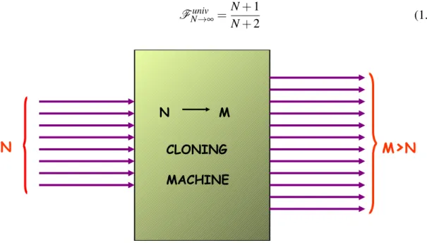
Figure 1.6: Universal cloning machine: the state |ψ⟩ is re-produced into the states|A⟩ and

|B⟩, the ancilla is represented

by the cloning machine in the state|C⟩

Due to linearity:

|ψ⟩|C⟩ →α|Σ0⟩ +β|Σ1⟩ ≡ |Σ⟩. (1.53)

The fidelity of clones, which measures the superposition between the input state and the clone, is given by:

(29)

Quantum Cloning 29

It can be demonstrated that if FA(ψ) =FB(ψ) are independent of ψ [BcvH96], then

the quantum mechanics allows the existence of a cloning transformation able to obtain a fidelity equal to:

Funiv₌5

6 ≃ 0.833 (1.55)

for which the following relations hold:

|0⟩|C⟩ → |Σ0⟩ ≡ √ 2 3|00⟩AB|0⟩C+ √ 1 3|ψ +_⟩ AB|1⟩C, |1⟩|C⟩ → |Σ1⟩ ≡ √ 2 3|11⟩AB|1⟩C+ √ 1 3|ψ +_⟩ AB|0⟩C (1.56) where |ψ+⟩ = |01⟩+|10⟩√

2 . By tracing out the degrees of freedom of C, we found that the

states A, B remain in the joint state:

ρAB= TrC(Σ) = 2 3|00⟩⟨00| + 1 3|ψ +_⟩⟨_ψ+_| (1.57) Tracing out one of the two clones state:

ρA= TrBC(Σ) = 2 3|ψ⟩⟨ψ| + 1 6I, ρB= TrAC(Σ) = 2 3|ψ⟩⟨ψ| + 1 6I (1.58) where I is the identity operator. From the relations (1.58), we note that the two clones are in the same state , and with probability 2₃ are in the state|ψ⟩, while with probability

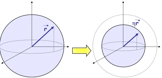
Figure 1.7: Cloning transformation reduces the state’s purity: the ray of the Bloch sphere is reduced by the shrinking factorη.

(30)

1

3 are in a complete mixed state I/2. This transformation can be represented graphically

through the Bloch sphere: the density matrix for a qubit can be written as in equation (1.19): with|−→r | = 1 for pure states. The depolarizing effect of the cloning process can be

thought as a reduction of vector −→r for a factorη, said shrinking factor, and the density matrix of the output state reads:

ρ′(r) =1 2(1 +η

−

→_r _{· −}→_σ₎ _(1.59)

η and the Fidelity of the cloning process are linked by the relation:

F = 1 +η

2 . (1.60)

1.5.2 Universal cloning N

→ M

Gisin and Massar [GM97] in 1997 introduced the concept of N → M cloning machine, able to transform N identical copy of an arbitrary state|ψ⟩⊗N into M > N identical clones. This process can be realized with a fidelity equal to:

Funiv N→M= M(N + 1) + N M(N + 2) = (N + 1) + N/M N + 2 (1.61)

When fixed N the number of clones increases, since the information has to be shared be-tween a greater number of partners, the Fidelity decreases. In the limit M→ ∞ the cloning transformation approaches the fidelity of the perfect measurement over N identical qubits in the state|ψ⟩⊗N [MP95]:

Funiv N→∞=

N + 1

N + 2 (1.62)

(31)

Quantum Cloning 31

1.5.3 Phase-covariant cloning

If we restrict our attention to a particular class of states, for instance the one that lay on the equatorial plane of the Bloch states:

|ϕ⟩ = |0⟩ + e√iϕ|1⟩

2 (1.63)

we obtain a value of the Fidelity greater respect to the universal cloning case.This is indeed the case of the phase covariant cloning process. The Fidelity results to be inde-pendent of the phase ϕ of the input qubit, and it has been demonstrated that its optimal value in the N→ M case is [Fen02]:

Fpc N→M= 1 2+ 1 M2N N−1

∑

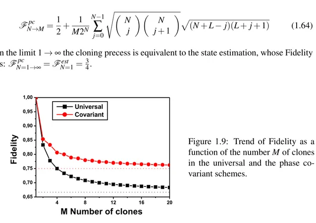
j=0 √( N j )( N j + 1 )√ (N + L− j)(L + j + 1) (1.64)

in the limit 1→ ∞ the cloning precess is equivalent to the state estimation, whose Fidelity is: F_N=1→∞pc =F_N=1est = 3₄.

Figure 1.9: Trend of Fidelity as a function of the number M of clones in the universal and the phase co-variant schemes.

In figure 1.9 a comparison between the trends of fidelity as a function of the number of clones, in the phase covariant and universal schemes, is reported. We see that the fi-delity value in the phase covariant case results to be higher than the universal one for each number of reproduced clones. This is due to the deeper knowledge about the state to be cloned, which spans only the equatorial plane of the Block sphere and not the over-all sphere itself, which characterize the phase covariant cloning process respect to the complete uncertainty about the state in a universal scheme.

(32)

(33)

Chapter 2 Theory of the Optical Parametric

Amplifier

The optical implementation of a qubit exploits the resources of both linear and non-linear optics. In this chapter we will show that quantum cloning can be implemented by the optical process of parametric down conversion.

We will address the concept of spontaneous-parametric-down-conversion (SPDC) in the context of non-linear optics, and the optical parametric amplifier, in both the collinear and non collinear configuration, will be characterized. The case of single photon amplification through a phase covariant amplifier will be then investigated in a more detail.

2.1 Elements of non-linear optics

The presence of radiation into an optical system can produce different changes inside the material, for instance in the index of refraction due to the electro-optic effect, or produce a variation in the radiation itself, as it happens in thesum anddifference-frequency gen-eration phenomena [Boy]. The interaction between the radiation and the system produce “non linear” phenomena, since the response of the material depends quadratically on the electromagnetic field.

In the linear case, the medium polarization P(t) is a function of the applied electric field

E(t):

P(t) =χ(1)E(t) (2.1)

whereχ(1) is the linear suscettivity.

In non-linear optics the response of the medium is expressed through a generalization of equation (2.1):

P(t) =χ(1)E(t) +χ(2)E2(t) +χ(3)E3(t) (2.2) whereχ(2) andχ(3)are the optical suscettivity at the send and third order respectively. The response of the medium can be considered instantaneous if the medium is not

(34)

34 Theory of the Optical Parametric Amplifier

sive and without losses, in this case the suscettivity is independent of the applied electric field’s frequency.

Sum and Difference-Frequency Generation (SFG) and (DFG) are examples of non linear second order processes, which happen in a non-centrosymmetric and non linear material, when a two-frequency (ω1andω2) incident field impinges on it:

E(t) = E1exp(−iω1t) + E2exp(−iω2t) + c.c. (2.3)

by considering only the second order term in equation (2.2), we obtain the expression of the second order polarization:

P(2)(t) =

∑

n

P(ωn) exp(−iωnt) (2.4)

where the sum over n is extended to negative and positive frequencies, and the ampli-tudes of different frequency components describe different physical phenomena: Sum-Frequency-Generation(SFG), Difference-Frequency-Generation (DFG), Second-Harmonic-Generation (SHG) (which is obtained when a radiation with frequencyωiis converted into

the second harmonic frequency 2ωi (with i = 1, 2) radiation) , and Optical-Rectification

(OR): P(2ω1) = χ(2)E12(t) (SHG) P(2ω2) = χ(2)E22(t) (SHG) P(ω1+ω2) = 2χ(2)E1(t)E2(t) (SFG) (2.5) P(ω1−ω2) = 2χ(2)E1(t)E2∗(t) (DFG) P(0) = 2χ(2)(E1E1∗+ E2E2∗) (OR)

Generally no more than one frequency component is present in the radiation after the interaction with the material, since each of the process described in equation (2.5) requires a different phase matching condition.

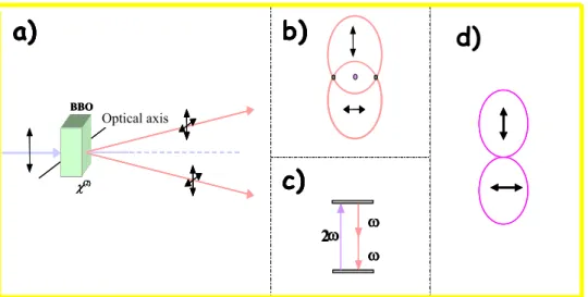
The difference between the processes of SFG e DFG is highlighted in figure 2.1:

in the SFG process two input photons at frequencyω1andω2are annihilated and a photon

at a greater frequencyω3is generated.

In DFG case for the energy conservation to generate a photon at frequencyω3, a photon

at greater frequencyω1must be destroyed and a photon at lower frequencyω2has to be

created.The DFG process amplifies the input field at the lowest frequency, for this reason it is also known as parametric amplifier.

According to the energy levels scheme, the DFG process can be described as follows: first an atom absorbs a photon at frequencyω1and jumps up to a virtual energy level which

decays emitting two photons; this process is stimulated by the presence of the input field at frequency ω2. Nevertheless the two-photon emission can happen even in absence of

(35)

Elements of non-linear optics 35

Figure 2.1: (a) Geometry of the SFG interaction. (b) Description of energy levels for SFG. (c) Geometry o9f the DFG interaction. (d) Description of energy levels for DFG. theω2field: in this case we have parametric fluorescence, and the process cannot be

(36)

2.2 Parametric Fluorescence

The parametric fluorescence phenomenon cannot be explained by classical theory but it is well described by quantum theory. As said, spontaneous parametric down conversion (SPDC) or parametric fluorescence is the nonlinear process whereby two photons (called idler and signal) are created from a parent photon (called the pump photon).

The interaction Hamiltonian between the radiation and the crystal reads:

H = 1 2 ∫ V d3r−→P · −→E = ∫ V d3r(χ_{i j}(1)EjEi+χ (2) i jkEjEkEi) (2.6)

If the pump field is intense, such as the one of the laser, it can be treated classically, while the field at frequencyω1andω2, calledsignal eidler, are quantized:

Ep=εp ∫ dkpexp(−4log2 [ωp(kp)− Ωp]2 σ2 p ) exp[kpz−ωp(kp)t] (2.7) b E(_j−)= i ∫ dkj √ ¯hjωj 2ε0n2(kj)Vba † − → kj exp(−i[kjzz +−→kj⊥· −→r⊥−ωj(kj)t]) (2.8)

where j = s, i, and ba†_j is the creation operator on spatial mode kj. The interaction

Hamil-tonian can then be written as: b H = C ∫ dkp ∫ dks ∫ dkiexp (−4log2[ωp(kp)−Ωp]2 σ2p )_expi(ωs+ωi−ωp) ∫ _L 0 dz× ×expi[kp−ksz−kiz]z ∫ A

d2r_⊥exp−i[−→k⊥i+−→k_⊥s]·−r→_⊥_ba†

− → ksba † − → ki + h.c. (2.9)

where C is a constant and L is the length of the crystal. The area A of the crossed transverse section can be considered infinite, since the transverse dimensions of the pump field are order of magnitude greater than the radiation wavelength. The integral in dr becomes then aδ(−→kp−→−ks −−→ki) function, responsible for one of the two phase-matching conditions of

the fluorescence process.

Since the second order interaction are considered to be weak, the exponential operator of the temporal evolution can be approximated with it’s first order expression:

b U (t) = exp ( −i ¯h ∫ _+∞ −∞ dt bH(t) ) ≃ I − i ¯h ∫ _+∞ −∞ dt bH(t) (2.10)

The dt integral in equation (2.9) gives then the second energy conservation condition:

δ(ωp−ωi−ωs). The two phase matching conditions express the necessity of conserving

both the energy and the momentum between the three fields:

ωp = ωs+ωi

− →

(37)

Parametric Fluorescence 37

Ifωi=ωs=1₂ωpwe talk about degenerate emission in frequency.

If the beams involved in the interaction are collinear, the condition of momentum conser-vation can be written as:

npωp c = nsωs c + niωi c (2.11)

this condition cannot be realized in linear crystals due to the normal dispersion phe-nomenon, for which the index of refraction increases monotonically with the radiation frequency. The use of anomalous dispersion regions makes the phase matching condition difficult to realize, due to the extreme variability of the index of refraction.

A better solution consists in using birefringent crystals, in which the index of refraction depends on the polarization of the impinging beam: an incident beam which makes an angleθ with the optical axis of the crystal experiences an index of refraction equal to:

1 ne(θ)2 = sin 2_θ n2 o +cos 2_θ n2 e

where neand noare the index of refraction extraordinary and ordinary seen by the

radia-tion propagating towards the direcradia-tions of the two optical axes.

For uniaxial crystals ne< no, it’s then more convenient to choose a pump beam at greater

frequency with extraordinary polarization, in this case signal and idler can have both the same polarization o (type I phase matching) or orthogonal polarizations (type II phase matching). In the first case the fluorescence is emitted over an ensemble of concentric cir-cumferences, each of which is given by photons with the same wavelength, the correlated photons (signal and idler) are in the diametrically opposite directions and on different cir-cumferences ifλi̸=λs.

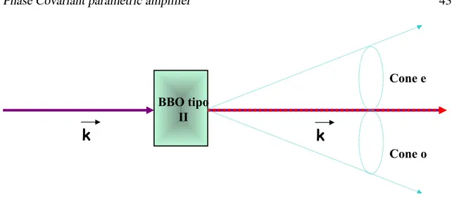
In type II phase matching case the photons are emitted over two non-coaxial cones, whose vertex is in the generation point of the parametric fluorescence inside the crystal and the aperture depends on the frequency (as shown in figure 2.2). One of the two cones contains photons with extraordinary polarization, the other the ones with ordinary polarization. If the emission is degenerate the two cones have the same aperture. The intersection be-tween them depends on the inclination of the pump beam respect to the optical axis of the crystal, and is responsible for the generation of entangled photons.

(38)

Figure 2.2: (a) Intersection between the ordinary and extraordinary cones. (b) Orthogonal polarizations of the generated beams. (c) Energy levels scheme in the degenerate fluo-rescence case, (d) Collinear case: entangled photons are generated over the same spatial mode.

2.3 The Optical Parametric Amplifier

The interaction between a radiation field at frequency ωp and a crystal with second

or-der non-linear suscettivity in oror-der to generate field at frequencies ω1 and ω2 such that

ω1+ω2=ωpcan be exploited by the optical parametric amplifier (OPA).

If the radiation fields have the same frequencies 2ω=ωpand are generated over the same

spatial mode the optical parametric amplifier is degenerate, if on the contrary the gener-ated fields are different in frequency or in spatial mode, the amplifier is non degenerate [WM94].

2.3.1 Degenerate amplifier

In a degenerate parametric amplifier the signal at frequency ω is amplified through the excitation of a crystal characterized byχ(2)̸= 0 with a beam at frequency 2ω. We consider the intense beam at frequency 2ω classically, while the one at frequency ω within the quantum theory, through the creation and destruction operator ba†andba.

The interaction Hamiltonian reads: b

H = ¯hωba†ba− i¯hχ

2(ba

2

e2iωt− ba† 2e−2iωt) (2.12) whereχ is proportional to the non linear suscettivity and to the pump beam’s amplitude. In the interaction picture we can write:

b

HI =−i¯hχ

2(ba

2_{− ba}† 2₎

(39)

The Optical Parametric Amplifier 39

and the Heisenberg motion equations are:

dba dt = 1 i¯h [ ba, bHI ] =χba† dba† dt = 1 i¯h [ ba†_{, b} HI ] =χba (2.14)

These equations have the following solution:

ba(t) = ba(0)cosh(χt) +ba†(0) sinh(χt) (2.15) The expression of the destruction operator’s solution reminds to the one of squeezing generator, the light produced by the parametric amplifier will then be squeezed. This can be verified by introducing the quadratures operator, and looking at their time evolution:

b X1 = ba+ ba† b X2 = ba− ba † i (2.16)

The equation which describe the quadratures’ motion are:

d bX1

dt = χXb1 d bX2

dt = −χXb2 (2.17)

These equations demonstrate that the parametric amplifier is phase sensitive, since a quadrature is amplified while the other is attenuated:

b

X1(t) = eχtXb1(0)

b

X2(t) = e−χtXb2(0) (2.18)

the temporal evolution operator bU = e−i bHIt/¯h _{coincides with the squeezing operator,} fur-thermore the mean number of generated photons, obtained with the injection of vacuum state is:

⟨bn⟩ = ⟨ba†_(t)_{ba(t)⟩ = sinh(g)}2 _(2.19)

with g =χt gain of the amplifier. The expression (2.19) correspond to the mean number

(40)

2.3.2 Non degenerate amplifier

In the non degenerate amplifier case, the classical field at frequency 2ω interacts with a non linear medium and generates two fields at frequencyω1andω2, such thatω1+ω2=

2ω over two spatial modes−→k1 and−→k2 called signal and idler.

The Hamiltonian of the system reads: b

H = ¯hω1ba†₁ba1+ ¯hω2ba†₂ba2+ iχ¯h(ba†₁ba†₂e−2iωt− ba1ba2e2iωt) (2.20)

where ba1 andba2 are the annihilation operator for signal and idler. The motion equations

in the interacting picture are:

dba1 dt = χba † 2 dba†₂ dt = χba1 (2.21)

and the solutions are:

ba1(t) = ba1cosh(χt) +ba†2sinh(χt)

ba2(t) = ba2cosh(χt) +ba†1sinh(χt) (2.22)

the number of generated photons is given by:⟨ bn1⟩ = ⟨ bn2⟩ = sinh(g)2.

2.4 Correlation functions

The classical optics interferometric experiments correspond to a measurement of the first order correlation function of the radiation field [Lou00]. Given two fields temporally sep-arated for a time intervalτ, a first order correlation function g(1)(τ) can be defined as:

g(1)(τ) =⟨E

∗_{(t)E(t +}_τ₎_⟩

⟨E∗_(t)E(t)_⟩ (2.23)

this coherence value gives an extimation of the fringe pattern visibilityV :

V = |g(1)

(τ)| 0 ≤ |g1(τ)| ≤ 1 (2.24) then completely coherent light, such as the laser one, has g(1)(τ) = 1, while for chaotic light g(1)(τ)→ 0 asτincreases.

In terms of quantized fields g(1)refers to the estimation of the average number of photons contained in the radiation:

(41)

Correlation functions 41

a first order coherence measurement of the radiation field coincides then with the extima-tion of the mean number of photons.

The study of second order correlation functions allows to distinguish between quantum and classical fields, which cannot be discriminated between a measurement of first order correlation one.

The second order correlation function is defined as:

g(2)(τ) = ⟨E

∗_(t)E∗_{(t +}_τ_{)E(t +}_τ_)E(t)_⟩

⟨E∗_(t)E(t)_⟩⟨E∗_{(t +}_τ_{)E(t +}_τ₎_⟩ (2.26)

in terms of quantized fields it reads:

g(2)(τ) =⟨ba

†_ba†_baba⟩

⟨ba†ba⟩2 =

⟨bn(bn− 1)⟩

⟨bn⟩2 (2.27)

for number state:

g(2)(τ) = {

(n− 1)/n se n≥ 2

0 se n = 0 (2.28)

it is worth noting that, while for classical light 1≤ g(2)(τ)≤ ∞, for quantum light 0 ≤

g(2)(τ)≤ ∞.

Another interesting physical quantity is the two modes correlation function, which can be addressed by analyzing the two different modes 1 and 2 at the exit of the amplifier:

g(2)₁₂(τ) = ⟨ba † 1ba † 2ba2ba1⟩ ⟨ba† 1ba1⟩⟨ba † 2ba2⟩ (2.29) generally the mixed correlation function follows the Cauchy-Schwartz inequality:

[ g(2)₁₂(0) ] ≤ g(2) 1 (0)g (2) 2 (0) (2.30)

in the quantum case a more strict inequality holds [WM94], which implies a greater cor-relation between the two spatial modes:

g(2)₁₂(0)≤ g(2)₁ + 1

⟨ba† 1ba1⟩

Generation and manipulation of multiphoton quantum fields

Universit´a degli Studi di Roma Tre

e

Consorzio Nazionale Interuniversitario per le

Scienze Fisiche della Materia

Dottorato di Ricerca in Scienze Fisiche della Materia

XXIII ciclo

Contents

I

Preliminary notions

11

II

Generation of multiphoton quantum states

49

III

Manipulation of multiphoton quantum states

101

IV

Applications

135

Introduction

Part I

Preliminary notions

Chapter 1

Elements of Quantum Information

1.1

Quantum states and their representation

1.1.1

Density matrix

∑

∑

1.1.2

Bloch sphere

1.2

Measurement and evolution of quantum states

1.2.1

Orthogonal measurements

∑

1.2.2

Generalized measurements

∑

1.2.3

Geometric representation

1.3

Entanglement

∑

∑

∑

∑

∑

1.4

Bell’s inequalities

1.5

Quantum Cloning

1.5.1

Optimal Universal Cloning

1.5.2

Universal cloning N

→ M

1.5.3

Phase-covariant cloning

∑

Chapter 2

Theory of the Optical Parametric

Amplifier

2.1

Elements of non-linear optics

∑

2.2

Parametric Fluorescence

2.3

The Optical Parametric Amplifier

2.3.1

Degenerate amplifier

2.3.2

Non degenerate amplifier

2.4

Correlation functions