2020-07-06T05:09:26Z
Acceptance in OA@INAF
Accurate estimators of correlation functions in Fourier space
Title
SEFUSATTI, Emiliano; Crocce, M.; Scoccimarro, R.; Couchman, H. M. P.
Authors
10.1093/mnras/stw1229
DOI
http://hdl.handle.net/20.500.12386/26334
Handle
MONTHLY NOTICES OF THE ROYAL ASTRONOMICAL SOCIETY
Journal
460
Number
Accurate estimators of correlation functions in Fourier space
E. Sefusatti,
1,2‹M. Crocce,
3R. Scoccimarro
4and H. M. P. Couchman
51INAF - Osservatorio Astronomico di Brera, via E. Bianchi 46, I-23807 Merate (LC), Italy 2INFN - Sezione di Padova, via Marzolo 8, I-35131 Padova, Italy
3Institut de Ci`encies de l’Espai, IEEC-CSIC, Campus UAB, Carrer de Can Magrans, s/n, E-08193 Bellaterra, Barcelona, Spain 4Center for Cosmology and Particle Physics, Department of Physics, New York University, New York, NY 10003, USA 5Department of Physics and Astronomy, McMaster University, Hamilton, ON L8S 4M1, Canada
Accepted 2016 May 19. Received 2016 May 18; in original form 2016 January 13
ABSTRACT
Efficient estimators of Fourier-space statistics for large number of objects rely on fast Fourier transforms (FFTs), which are affected by aliasing from unresolved small-scale modes due to the finite FFT grid. Aliasing takes the form of a sum over images, each of them corresponding to the Fourier content displaced by increasing multiples of the sampling frequency of the grid. These spurious contributions limit the accuracy in the estimation of Fourier-space statistics, and are typically ameliorated by simultaneously increasing grid size and discarding high-frequency modes. This results in inefficient estimates for e.g. the power spectrum when desired systematic biases are well under per cent level. We show that using interlaced grids removes odd images, which include the dominant contribution to aliasing. In addition, we discuss the choice of interpolation kernel used to define density perturbations on the FFT grid and demonstrate that using higher order interpolation kernels than the standard Cloud-In-Cell algorithm results in significant reduction of the remaining images. We show that combining fourth-order interpolation with interlacing gives very accurate Fourier amplitudes and phases of density perturbations. This results in power spectrum and bispectrum estimates that have systematic biases below 0.01 per cent all the way to the Nyquist frequency of the grid, thus maximizing the use of unbiased Fourier coefficients for a given grid size and greatly reducing systematics for applications to large cosmological data sets.
Key words: methods: analytical – methods: data analysis – methods: numerical – methods:
statistical – large-scale structure of Universe.
1 I N T RO D U C T I O N
A great effort is currently directed towards accurate measurements of the power spectrum of the galaxy distribution as a test of the cosmological model (see e.g. Laureijs et al.2011; Levi et al.2013). At the same time, theoretical predictions for the matter and galaxy power spectrum, which play a key role in the interpretation of observational data, are ultimately validated by measurements of such quantities in numerical simulations. Due to computational efficiency, Fourier-space statistics in simulations and galaxy sur-veys are usually computed using fast Fourier transforms (FFTs), which require building estimates of density or galaxy perturbations on a regular grid from the input data objects (N-body particles or galaxies). These Fourier coefficients are then used to calculate cor-relation functions in Fourier space such as the power spectrum or bispectrum.
⋆E-mail:[email protected].
However, introducing a discrete sampling as the FFT grid comes with limitations that can only be avoided under special circum-stances. If the underlying spectrum of perturbations is bandwidth limited (vanishes above a cutoff frequency kmax), then the sampling
theorem guarantees that grid estimates are lossless as long as the sampling frequency of the grid (ks= 2π/H , where H is the grid
spacing) is at least twice the cutoff frequency, ks≥ 2kmax. This just
says that the grid is fine enough so that every Fourier component in the signal is sampled at least twice per period, which intuitively makes sense (at least a peak and a trough is needed to resolve an oscillation).
Unfortunately, the conditions of the sampling theorem are not sat-isfied by cosmological perturbations, which have significant Fourier content at all frequencies. As a result of this, unresolved small-scale modes when sampled by the grid are mistakenly identified as modes supported by the grid, which results in spurious contamination of the FFT-determined Fourier coefficients that directly translates into a systematic error in e.g. the power spectrum and bispectrum. This contamination is known as aliasing: it takes the form of a sum over
at SISSA on October 12, 2016
http://mnras.oxfordjournals.org/
images, each of them corresponding to the Fourier content displaced by increasing multiples of the sampling frequency of the grid ks, as we shall discuss in detail below.
Aliasing can be removed entirely if the signal is first low-pass filtered so that only frequencies supported by the grid remain be-fore sampling by the grid, effectively making the modified signal bandwidth limited. Although such process is not lossless (high fre-quencies are missing), the determination of the supported Fourier modes is free of systematics. Low-pass filtering, however, results in interpolating kernels that are very non-local in real space (a given object contributes to essentially all grid points), and thus the def-inition of perturbations on the grid becomes too computationally expensive to be useful despite the speedup of FFTs. The goal to minimize aliasing is therefore to design an interpolating kernel that is fairly local while at the same time acts as much as possible as a low-pass filter (i.e. it is fairly smooth). In this paper, we present an algorithm that achieves this for realistic spectra of cosmologi-cal perturbations. By working at the level of the Fourier modes, it simultaneously benefits all Fourier-space statistics.
The issue of aliasing in the measurements of the power spectrum has been addressed, in the specific context of cosmological studies, by Jing (2005), Cui et al. (2008), Yang et al. (2009), Colombi et al. (2009) and Jasche, Kitaura & Ensslin (2009). In particular, Jing (2005) derives the full expression, including the aliasing compo-nent, for the power spectrum measured from interpolation on a grid with a generic mass assignment scheme and proposes an iterative procedure to reduce the aliasing contribution based on the exact knowledge of the window function in Fourier space corresponding to such scheme. Cui et al. (2008) and Yang et al. (2009) do not attempt to correct for the error introduced by aliasing but search instead for an optimal assignment scheme able to reduce the ef-fect. They identify for this purpose the scaling function of specific Daubechies wavelets and claim, as a result, a systematic error be-low the 2 per cent level for wavenumbers k < 0.7kNyq, kNyq≡ ks/2
being the Nyquist frequency of the grid. A different approach is explored by Colombi et al. (2009) who consider a Fourier–Taylor expansion of the expression corresponding to a direct summation of the particle contribution to the density field in Fourier space. At the lowest order the procedure, implemented in thePOWMES
pub-lic code, corresponds to a Nearest Grid Point (NGP) assignment scheme but including higher order corrections it quickly converges to an unbiased estimator of the power spectrum, albeit at signif-icant computational cost. Finally, Jasche et al. (2009) discuss a method based on ‘supersampling’ that inevitably increases memory requirements (typically by almost an order of magnitude).
In this paper, we revisit a technique based on interlacing two density grids that, while requiring only two times the number of density evaluations w.r.t. the standard case, can significantly reduce the aliasing contribution. The method is discussed in Hockney & Eastwood (1981), and has been implemented in the AP3M N-body
code for the mesh force calculation in Couchman (1991, see also Couchman1999). Here, we show how it can be applied to the eval-uation of the density field in Fourier space from point distributions. In particular, we quantify the relative effect of different mass assign-ment schemes on the aliasing contributions to the power spectrum estimation in two typical situations of cosmological interest: the non-linear matter distribution at low redshift from a small N-body simulation and the matter distribution obtained in the Zeldovich approximation (ZA) at high redshift. We proceed to illustrate the interlacing technique and we compare our results to Fourier co-efficient evaluations by direct summation over objects (which are alias-free) and to the output of thePOWMESpublic code.
The paper is organized as follows. Section 2 introduces and de-scribes the problem of aliasing in mathematical terms, with specific attention to its interplay with the order of the mass assignment scheme adopted. Section 3 presents the interlacing technique and its effect on different power spectrum measurements. In Section 4, we quantify the contribution of aliasing with and without interlac-ing to higher order correlation functions such as the bispectrum. We present our conclusions in Section 5.
2 D E N S I T Y E S T I M AT I O N A N D A L I A S I N G 2.1 Correlation functions in Fourier space
We focus our attention on continuous fields defined over a finite, cubic volume V = L3which we will assume equivalent to the case
of infinite volume but periodic with period L along each of the three spatial directions (the extension to the general case of a generic box of different periods while trivial, would require a significantly more cumbersome notation).
The matter density ρ(x) can be described in terms of the dimen-sionless overdensity
δ(x) ≡ ρ(x)
¯ρ −1, (1)
where ¯ρ is the mean density in the volume V. Its Fourier space counterpart is given by δ(k) ≡ ! V d3x (2π)3e−ik·xδ(x), (2)
while its inverse is defined in terms of the series δ(x) ≡ k3f "
k
eik·xf(k), (3)
since k is discretized in multiples of the fundamental frequency kf = 2π/L in each spatial direction. Notice that we will always
explicitly show the argument of each function in order to distinguish a real-space object from its Fourier transform.1
The power spectrum P(k) is then defined as the two-point function of δ(k), that is ⟨δ(k1) δ(k2)⟩ ≡ δK k12 k3f P(k1), (4)
with ⟨ . . . ⟩ representing the ensemble average, ki1,...,in≡ ki1+
· · · + kin and δ K
k being a Kronecker delta defined to be equal to 1 for a vanishing argument k = 0 and zero otherwise. Similarly, the bispectrum B(k1, k2, k3) is defined as ⟨δ(k1) δ(k2) δ(k3)⟩ ≡ δK k123 k3f B(k1, k2, k3). (5)
In this convention, the continuous limit is recovered for V → ∞ or kf→ 0 with δKk/kf3→ δD(k), the latter being a Dirac delta function. 2.2 Direct summation
Theoretical predictions for the correlation functions of the mat-ter density, or of the galaxy number density, often assume such
1In this convention for the Fourier transform, the Dirac delta in real space
and the Kronecker delta in Fourier space are given, respectively, by the following representations: δD(x) =V1 # k eik·x and δK k = V1 $ d3xe−i k·x. at SISSA on October 12, 2016 http://mnras.oxfordjournals.org/ Downloaded from
quantities to be continuous random fields. However, in practical applications such as the analysis of N-body simulations or galaxy surveys they are given in terms of a finite number NP of objects
with positions {xi} for i = 1, . . . , NP. In this case, we can write the
density as ρ(x) = NP " i=1 m δD(x − xi), (6)
mbeing the particle mass which we assume here to be the same for all particles, for simplicity. It follows that
δ(x) = 1 ¯n NP " i=1 δD(x − xi) − 1, (7)
¯n ≡ NP/V being the particle density. The overdensity in Fourier space can be obtained by direct summation as the Fourier transform of the equation above, that is
δ(k) = 1 (2π)3 % 1 ¯n NP " i=1 e−i k·xi− VδK k & . (8)
The Fourier-space two-point function defining the power spectrum is now given by ⟨ δ(k1) δ(k2) ⟩ = δK k12 kf3 ' P(k1) + 1 (2π)3¯n ( , (9)
where the second term on the r.h.s. represents the shot-noise con-tribution due to the self-correlation of individual particles (see for instance, Peebles1980; Jing2005). The direct summation estimator for the power spectrum of a particle distribution is then
ˆP (k) ≡ k3 f|δ(k)|2= kf3 ' |δ(k)|2− 1 NP ( , (10)
and the true power spectrum is recovered as P (k) = ⟨ ˆP (k)⟩. Direct summation is clearly quite a demanding approach, partic-ularly in the case of N-body simulations with a very large number of particles, since the evaluation of the Fourier-space density scales as NP× NG3, NG3 being the number of wavenumbers k required.
While impractical, it is however an exact alias-free determina-tion of Fourier coefficients. Therefore, we shall use direct sum-mation estimates below as a benchmark to which FFT methods are compared.
2.3 Mass assignment and aliasing
A more efficient method, taking advantage of the FFT algorithm, requires first the interpolation of the density field on a regular grid in position space. This fixes the largest wavenumber accessible to the Nyquist frequency, kNyq= πNG/L = π/H, NGbeing now the linear
size of the grid and H = L/NGtherefore being the grid spacing. The
price to pay is the emergence of aliasing in the Fourier transform of the density grid and therefore a systematic error that cannot be easily and completely removed from the measurements of the correlation functions in Fourier space. We will loosely revisit here the derivation by Jing (2005) of the theoretical expression for the power spectrum estimator based on grid interpolation and the FFT, since it will be useful to describe the interlacing method discussed in Section 3.
Let us assume xG
j with j = 1,...,NG3to be a regular grid of points,
for simplicity, linearly spaced by H in all directions. The interpo-lation of a continuous function f (x) over the grid can be given by
a simple integration over the cell of volume H3surrounding each
point, so that f(xGj) = 1 H3 ! xG j d3x f(x) ≡ 1 H3 ! xG j+H /2 xG j−H /2 dx ! yG j+H /2 yG j−H /2 dy! zG j+H /2 zG j−H /2 dz f (x) . (11) In the case of the density defined by a particle distribution as in equation (6), each particle will provide a contribution only to the cell encompassing the particle position. As we will see, this simple procedure, known as the NGP assignment scheme, is not the optimal one. To consider more general schemes, it is convenient to assign a ‘shape’ to each particle defined by a function S(x) which is sym-metric, positive defined, separable as S(x) = S1D(x) S1D(y) S1D(z),
and normalized such that$d3xS(x)/(2π)3= 1. Separability makes computations efficient, since the resulting scheme will only need 1D distances in each direction, as opposed to e.g. spherically symmet-ric shapes which require radial distances to be computed. Similarly, correcting for the interpolation window in Fourier space is straight-forward when separability is assumed.
The interpolation over the grid corresponds then to the evaluation of the (continuous) function
)δ(x) ≡! (2π)d3x′3W(x − x′) δ(x′) (12)
at the grid points xG
j, leading to )δ(xG j) = 1 (2π)3¯n NP " i=1 W*xGj − xi + − 1, (13)
where the weight function W (x) is simply the integral over the cell volume of the shape function S(x) given by
W(xG j − xi) = 1 H3 ! xG j d3x S(x − xi) . (14)
In addition to the NGP, assignment schemes commonly adopted are the Cloud-In-Cell (CIC) and Triangular Shape Cloud (TSC) scheme, representing the lowest order piecewise polynomial func-tion (also known as B-splines). They correspond, respectively, to first, second and third order referring to the number p of grid points, per dimension, to which each particle is assigned. The relative piecewise polynomial functions W(p)are of order less or
equal to (p − 1), and correspond simply to convolving a top-hat function with itself (p − 1) times. The weights are then given explicitly by W (x) = W(p)(x/H ) W(p)(y/H ) W(p)(z/H ),
where for each different scheme we have the one-dimensional functions: (i) NGP W(1)(s) = , 1 for |s| < 1 2 0 otherwise (15) (ii) CIC W(2)(s) = , 1 − |s| for |s| < 1 2 0 otherwise (16) (iii) TSC W(3)(s) = ⎧ ⎪ ⎨ ⎪ ⎩ 3 4− s2 for |s| < 1 2 1 2 *3 2− |s| +2 for1 2≤ |s| <32 0 otherwise, (17) at SISSA on October 12, 2016 http://mnras.oxfordjournals.org/ Downloaded from
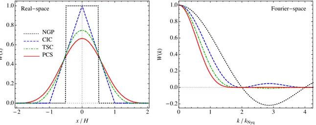
Figure 1. Left-hand panel: one-dimensional, real-space window functions W(p)(x) of the four mass assignment schemes described in the text. Different curves
show NGP (dotted, black), CIC (dashed, blue), TSC (dot–dashed, green) and PCS interpolation (continuous, red). Right-hand panel: the same window functions in Fourier space, W(p)(k).
where s = (xG
j − x)/H . Clearly, schemes of order higher than TSC
can be considered (as it is often the case in plasma physics appli-cations, see e.g. Haugbølle, Frederiksen & Nordlund2013). Here, we will consider only the next, fourth-order interpolation scheme, which we will refer to as Piecewise Cubic Spline (PCS; see e.g. Chaniotis & Poulikakos2004, for generic, higher order B-spline interpolation). The corresponding weights are given by
(i) PCS W(4)(s) = ⎧ ⎪ ⎨ ⎪ ⎩ 1 6 * 4 − 6 s2+ 3 |s|3+ for 0 ≤ |s| < 1 1 6(2 − |s|) 3 for 1 ≤ |s| < 2 0 otherwise. (18)
In the left-hand panel of Fig.1, we show the one-dimensional window functions in real space W(p)(x) where it is evident how the
support of the weight function grows with the interpolation order. The sampling in real space given by equation (13) can be math-ematically described in terms of the sampling function Ш (x) (see e.g. Hockney & Eastwood1981). This is defined as
Ш(x) =" n
δD(x − n), (19)
with n an integer vector. It is easy to see that the Fourier transform of )δ(xG
j) is equal to the Fourier transform of the continuous field
given by the product Ш(x/H ) )δ(x) which is different from zero only for x = xG
j and equals )δ(xGj) at those points when integrated
over. Applying the convolution theorem, we obtain )δG(k) = k3
f
" k′
Ш(k′) )δ(k − k′), (20)
where )δ(k) is the Fourier transform of the convolved, continuous density field defined in equation (12), while )δG(k), in addition,
accounts for the discreteness of the grid assignment.
We notice now that the Fourier transform of the sampling function is a sampling function in k-space. Since we are dealing with periodic functions in position space, the Delta functions are replaced by Kronecker deltas as Ш(k) = 1 kf3 " n δK k−n ks, (21)
where the sampling frequency of the grid ksis given by ks≡ 2π H (22) so that we obtain )δG(k) =" n )δ (k − n ks) , (23)
where clearly )δGis ks-periodic and we are thus interested in
frequen-cies |k| ≤ ks/2 = kNyq= π/H = π NG/L, with kNyqthe Nyquist
frequency of the grid. In this expression, all terms with n ̸= 0 in the sum represent the aliasing contribution to the estimate )δG(k) of the
density )δ(k), which, we should keep in mind, includes the effect of the interpolation function W (x). Such effects can be removed from the leading contribution in the sum above, simply dividing by the FT of the window function itself, W (k). The corrected, grid-based density contrast would then be given by
δG(k) ≡)δ G(k) W(k) = 1 W(k) " n )δ (k − n ks) , (24)
and introducing the ‘corrected’ window function wn(k) ≡W(k − n ks)
W(k) , (25)
defined in such a way that w0(k) = 1, we obtain
δG(k) = δ (k) +" n̸=0
wn(k) δ (k − n ks) , (26)
where indeed the n = 0 term provides the desired estimation of the density δ(k), while all other terms correspond to spurious, aliasing contributions. They correspond to ‘images’ of the Fourier content δ(k) centred at increased multiples of the sampling frequency of the grid ks. For the frequencies of interest, |k| ≤ ks/2 = kNyq, the
images correspond to small-scale modes not supported by the grid that masquerade as modes of the frequency range we are interested in. These unwanted contributions have an amplitude that depends not only on the small-scale power but also on the weight given by the corrected window function wn.
Our main goal here is therefore to minimize wnsubject to the constraints of computational speed. Ideally, as pointed out in the
at SISSA on October 12, 2016
http://mnras.oxfordjournals.org/
introduction, to remove aliasing one would choose an interpolation function W(k) which is a low-pass filter for modes of frequency less than ks, which would automatically make the wnvanish. The drawback of this choice is that the real-space kernel is then very non-local and that makes inefficient the interpolation to the grid, since each object would contribute to a large number of grid points. This, in effect, would constitute the bottleneck of the computational cost, and would negate the whole point of using FFTs as opposed to direct summation. The objective is then to find interpolation kernels that are sufficiently local in both real and Fourier space.
In order to highlight these aspects, on the right-hand panel of Fig.1we show the (one-dimensional) window functions in Fourier space W(k). For the B-spline windows considered above these are simply given by W(p)(k) =' sin(kH/2) (kH /2) (p =' sin(π k/k(π k/k s) s) (p , (27)
p = 1–4 being the interpolation order corresponding to NGP, CIC, TSC and PCS. Again, equation (27) makes clear that the different interpolation schemes correspond to convolutions of (p − 1) top-hat functions in 1D. For the 3D case, due to the separability assumption, one simply multiplies three such objects for each dimension, which is quite efficient. It is clear from Fig.1that the PCS kernel satisfies the opposite requirements of compactness in real and Fourier space rather well, although there is of course a tradeoff. The Fourier-space compactness means that the amplitude of the unwanted images wn will be highly suppressed, this comes at the expense of a slightly more expensive interpolation to the grid as the real-space kernel is correspondingly broader. We will examine the impact of these choices for the power spectrum and bispectrum below.
As mentioned above, any aliasing correction to the density field will inevitably affect the estimation of any correlation function. In the first place, the two-point function of the interpolated, corrected density field δG(k), will be given by
⟨ δG(k1) δG(k2) ⟩ =
" n1,n2
wn1(k1) wn2(k2)
× ⟨ δ(q1) δ(q2) ⟩, (28)
where qi= ki− niksand where the expectation value on the r.h.s.
coincides with the one of equation (9).
The relation between the power spectrum estimated from the grid-based density δGand the desired power spectrum P(k) of the
original distribution is then given by PG(k) ≡ kf3⟨ |δG(k)|2⟩
=" n
|wn(k)|2Ptot(|k − n ks|) , (29)
where Ptot(k) ≡ P (k) + 1/[(2π)3¯n], an expression first derived by
Jing (2005), here corrected for the window effects at leading order in the aliasing expansion.
In the case of the bispectrum BG(k
1, k2, k3), we obtain the similar
expression, BG(k1, k2, k3) = " n1,n2,n3 wn1(k1) wn2(k2) wn3(k3) × δK q123Btot(q1, q2, q3) = " n1,n2 wn1(k1) wn2(k2) w−n12(−k12) × Btot(k1− n1ks,k2− n2ks), (30) where Btot≡ B(k1, k2, k3) + 1 (2π)3¯n[P (k1) + P (k2) + P (k3)] +(2π)16¯n2, (31)
and where, again, only the leading term for n1= n2= n3= 0
corresponds to the desired estimated bispectrum (plus shot-noise), while all the others provide unwanted aliasing contributions.
Jing (2005) proposes a procedure to correct for the aliasing con-tribution to the power spectrum by means of a function that requires, in principle, a priori knowledge of the target power spectrum itself. Since, however, such knowledge is relevant only for values close to the Nyquist frequency, a power-law approximation of the power spectrum, determined by an iterative scheme, is employed instead. While this could provide a reasonable and effective solution to the problem of aliasing in power spectrum estimation, the procedure cannot be easily extended to the bispectrum, where one would need a model to describe the scale and triangle-shape dependence of high-k modes to effectively handle such corrections.
We will explore, in the rest of the paper, a more flexible alternative.
3 A L I A S I N G R E D U C T I O N B Y I N T E R L AC I N G 3.1 Interlacing
A method to partially correct for aliasing based on the interlacing of two grid is discussed in Hockney & Eastwood (1981), and its implementation in the AP3M N-body code by Couchman (1991) for
the mesh force calculation is mentioned in Couchman (1999). We have seen that, for a generic mass assignment scheme, the interpolated density field, denoted below as )δG
1(k), can be written
as in equation (23), which we reproduce here for convenience )δG 1(k) = ! V d3x (2π)3e−i k· xШ 1 x H 2 )δ(x) =" n )δ (k − n ks) . (32)
An additional, real-space interpolation on a grid shifted by the distance H/2 in all spatial directions, with respect to the one above can be written as )δG 2(k) = ! V d3x (2π)3e−i k· xШ 3 x H + 1 2 4 )δ(x) . (33)
Again, since this represents the FT of a product, it can be written as a convolution of Fourier series, where, this time, the transform of the sampling function, equation (21), is obtained taking advantage of the shift theorem so that
)δG 2(k) = k3f " k′ e−i (k′ x+ky′+k′z) H /2Ш(k′) )δ(k − k′) =" n e−π i (nx+ny+nz))δ (k − n k s) =" n (−1)nx+ny+nz)δ (k − n k s) . (34)
Considering now the linear combination of the two, one obtains )δG(k) =1 2 5 )δG 1(k) + )δ2G(k) 6 =" n θn)δ (k − n ks) , (35) at SISSA on October 12, 2016 http://mnras.oxfordjournals.org/ Downloaded from
where we defined θn≡ 1 2 7 1 + (−1)nx+ny+nz8 = , 1 for nx+ ny+ nzeven 0 for nx+ ny+ nzodd. (36) In the expression of equation (35) for the interlaced density all aliasing contributions (images) corresponding to odd values of the sum nx+ ny+ nz, including, in particular, the largest ones for |n| =
1 are removed. Clearly, the density field thus obtained should still be corrected for the effects of the window function as in equation (24), so that δG(k) = )δG(k)/W (k). In principle, the scheme could be
extended to the combination of more than two interpolated density grids to remove the leading aliasing contributions at the next order. The power spectrum of the interlaced density field, corrected for the window function, can now be written as
PG(k) =" n
θn|wn(k)|2Ptot(|k−n ks|) , (37)
while the expression for the power spectrum of the (not interlaced) field of equation (29) is then recovered substituting θnwith 1 in the equation above.
We can write the residual aliasing contribution as &PG(k) ≡ PG(k) − Ptot(k)
=" n̸=0
θn|wn(k)|2Ptot(k − n ks) . (38)
Assuming that, for all k > kNyq, the power spectrum has an upper
bound Pmax≥ P(k), the residual is, in turn, bounded as
&PG(k) ≤ ' Pmax+ 1 (2π)3¯n ( Fres(k), (39)
where we introduce the residual factor Fres(k) on the r.h.s., defined
as Fres(k) ≡
" n̸=0
θn|w2n(k)|2. (40)
For mass assignment schemes corresponding to B-splines as those considered before, it is possible to evaluate this residual factor explicitly. For the interpolation order p, we have
Fres(x) = " n̸=0 θn 3 9 i=1 3 x i xi− ni 42 p , (41)
where x ≡ k/ksand the product runs over the three spatial
dimen-sions. With no interlacing we obtain, more simply Fres(x) = " n̸=0 3 9 i=1 3 x i xi− ni 42 p . (42)
We note that in these expressions, a relatively small number of terms are enough to recover a reasonable accuracy.
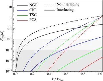
Fig.2shows, for simplicity in one spatial dimension, the function Fres(k) for the four interpolation schemes assumed in the previous
section, evaluated with and without interlacing. The figure nicely illustrates both the effects due to the choice of the interpolation scheme and due to the interlacing procedure. In the interlacing case, the 1D residual function explicitly corresponds to
Fres,1Dint (x) = " n̸=0 3 x x− 2 n 42 p =1 x222p [ζ (2 p, x/2) + ζ (2 p, −x/2)] − 2, (43)
Figure 2. Residual factor Fres, 1D(k), in one spatial dimension, as a function
of the ratio of the wavenumber k to the Nyquist frequency, evaluated for the four interpolation schemes considered. Continuous and dashed curves assume, respectively, results with and without interlacing, equation (43) and equation (45), respectively.
where we introduced the Hurwitz zeta function ζ(p, x) = ∞ " n=0 1 (n + x)p. (44)
Without interlacing we have instead Fres,1Dno−int(x) = " n̸=0 3 x x− n 42 p = x2p [ζ (2 p, x) + ζ (2 p, −x)] − 2 . (45) We therefore obtain, in one dimension, the simple relation Fres,1Dint (x) = Fres,1Dno−int(x/2) . (46)
Fig.2indicates in particular, as we will show with numerical tests in the next sections, that without interlacing, the aliasing contribution reaches relevant values approaching the Nyquist frequency kNyq,
regardless of the mass assignment scheme chosen. With interlacing, according to equation (46), this will happen at k equal twice kNyq,
i.e. well outside the interval of interest.
In a similar way, we can write the bispectrum of the interlaced field as BG(k1,k2) = " n1,n2 θn1θn2θ−n12 × wn1(k1) wn2(k2) w−n12(−k12) × Btot(k1− n1ks,k2− n2ks), (47)
where the residual aliasing contributions correspond to all terms in the sums with n1̸= 0 and n1̸= 0. In this case, we could not find
a simple expression taking advantage of the explicit form of the B-spline window functions. We will present a numerical estimate of the aliasing contribution to the bispectrum in Section 4.
As a matter of fact, it is important to stress that the aliasing reduction is obtained, by interlacing, at the level of the density field, not after the power spectrum evaluation. As we will see, this fact ensures that the method benefits extend to all higher order correlations that can be estimated from the FT of field itself. Also,
at SISSA on October 12, 2016
http://mnras.oxfordjournals.org/
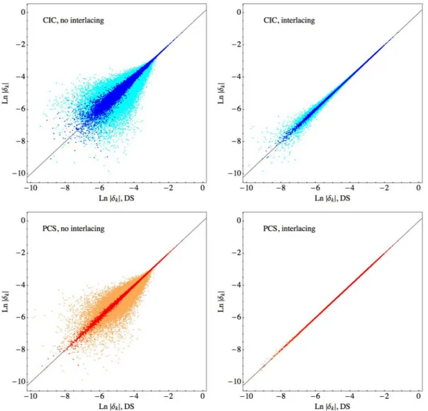
Figure 3. Scatter plots comparing the (log) amplitude of the Fourier-space density, ln |δ(k)| obtained by interpolation on a grid and the same quantity obtained
by direct summation. Top row assumes the CIC mass assignment scheme, while bottom row the PCS mass assignment scheme. Left-hand column assumes no correction by interlacing, while the right-hand column does. In all panels, light shaded (cyan and orange) points correspond to all modes in the grid of linear size NG= 100 while dark shaded (blue and red) points are restricted to modes of |k| ≤ 0.7 kNyq.
since interlacing only removes the odd images, it is important to supplement this technique with a reasonable choice of interpolation kernel as discussed in the previous section to suppress the amplitude of the remaining alias images.
3.2 Comparison to direct summation
The effects of aliasing are most effectively estimated comparing the density field in Fourier space obtained by a given interpolation scheme with the density field obtained by direct summation to the same grid, where they are absent. Along the lines of the tests pre-sented in Colombi et al. (2009), in this section we consider two different particle distributions both relevant for large-scale struc-ture studies: an N-body simulation evolved to redshift zero on a relatively small box (therefore characterized by significant non-linearities) and a distribution obtained in the ZA at high redshift. Due to the significant numerical resources required by the direct summation, we will consider distributions of a relatively low num-ber of particles.
For the N-body simulation, we make use of the controlled numer-ical experiment described in Colombi et al. (2009), run on a box of size L = 50 h Mpc−1of side with NP= 1283particles, and publicly
available in thePOWMESpackage as a test for the code.
In this case, before presenting the comparison between power spectra and to underline the fact that the interlacing correc-tion acts at the level of density field, we show a compari-son between the amplitudes (as ln |δ(k)|, Fig. 3) and phases (φ = arctan [Im δ(k) / Re δ(k)], Fig. 4) of the density in Fourier space. Since small-scales modes dominate the scatter plot due to their larger number, we show large-scale modes characterized by |k| ≤ 0.7 kNyqby a darker shade (red or blue in the colour figure),
while all others are denoted by a lighter shade (orange or cyan). While this is a rather qualitative comparison, it is evident that both the choice of the assignment scheme and the correction provided by interlacing play an important role in the reducing the scatter, and this is true for the amplitudes and phases alike. In particular, we can notice how the benefits of PCS interpolation and interlacing extend to all modes, all the way up to the Nyquist frequency, while in the other cases small scales are affected by a significant scatter.
at SISSA on October 12, 2016
http://mnras.oxfordjournals.org/
Figure 4. Same as Fig.3, but comparing the phases of the Fourier-space mode, φ = arctan [Im δ(k) / Re δ(k)].
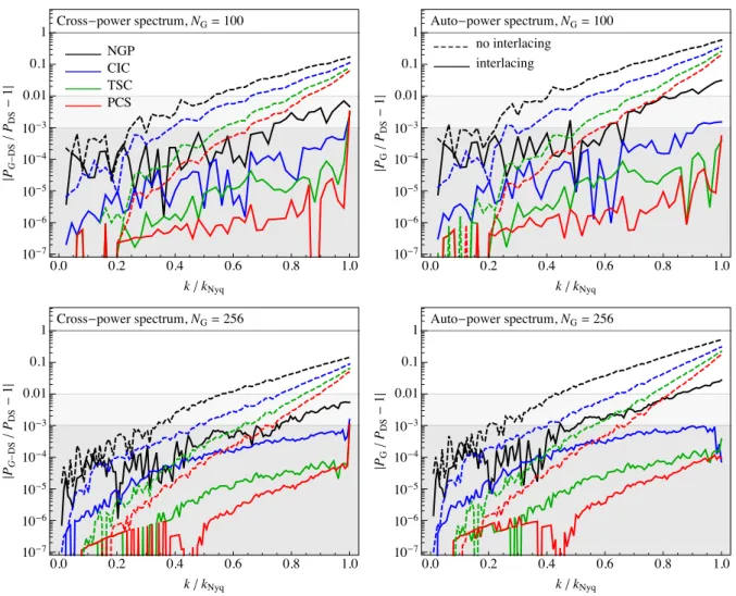
More quantitative results can be obtained by looking at measure-ments of the power spectra. Fig.5shows the comparison between the simulation power spectrum obtained by different mass assignment schemes and the one obtained by direct summation. In particular, the left-hand panel shows the absolute value of the relative difference between the cross-power spectrum obtained from the grid-based (and window-corrected) density field δG(k), with the one obtained
by direct summation, δ(k), that is PG−DS∼ ⟨δG(k) δ(−k)⟩, to the
autopower spectrum PDS∼ ⟨|δ(k)|2⟩, in short
: : : : PG−DS(k) PDS(k) −1 : : : : .
This quantity provides an estimate of the error induced on the den-sity field itself by the grid assignment and aliasing. The right-hand panel of Fig.5shows instead the relative difference between the autopower spectra PG∼ ⟨|δG(k)|2⟩ and PDS,
: : : : PG(k) PDS(k) − 1 : : : : ,
larger roughly by a factor of 2, as one can expect. Both auto-and cross-power spectra are corrected for shot-noise simply by subtracting the inverse number density of the box. Upper panels assume an interpolation grid of linear size NG= 100 while lower
panels assume NG= 256. In all cases, results are shown as a function
of the ratio of the wavenumber k to the Nyquist frequency kNyq
≡ π NG/L, L being the size of the box. In this way, it is easy
to read-off the reach in the range of validity of each interpolation scheme in terms of the relative fraction of the Nyquist. For instance, the commonly used CIC scheme, when no aliasing correction is applied, provides a per cent level accuracy only up to 0.6 kNyq.
The immediate consequence of this fact is that if per cent accuracy is required on a given range of scale, to avoid unwanted aliasing contributions the interpolation grid should be ∼6 (1/0.63, in three
dimensions) times larger than the one naively expected in the case such accuracy could be reached over all wavenumbers, resulting in much larger numerical effort. The situation is even worse if the required accuracy is at the 0.1 per cent level; in this case, the CIC reach is k ! 0.4 kNyq. Different, higher order interpolation
schemes can marginally improve the range of scales over which a given accuracy is recovered, but they show aliasing components converging to the same value (at tens of per cent level) as the Nyquist frequency is approached.
Such behaviour is significantly reduced, instead, when the inter-lacing technique is applied. In this case, a 0.1 per cent accuracy is reached, with a CIC scheme, all the way up to the Nyquist, while PCS provides 0.01 per cent accuracy at the Nyquist frequency and reaches the limits imposed by single precision arithmetic (∼10−7)
used in this test at low wavenumbers.
at SISSA on October 12, 2016
http://mnras.oxfordjournals.org/
Figure 5. Comparison between the power spectrum measured by FFT of a grid interpolated field and the same quantity obtained by direct summation
as a function of the wavenumber in units of the Nyquist frequency. The left-hand panel show the absolute value of the relative difference between the cross-power spectrum of the grid-based, window-corrected field with the direct summation density field, PG−DS∼ ⟨δG(k) δ(−k)⟩ to the autopower spectrum PDS∼ ⟨|δ(k)|2⟩. The right-hand panel shows instead the relative difference between the autopower spectra PG∼ ⟨|δG(k)|2⟩ and PDS. Results in the top panels
assume a (linear) FFT grid of NG= 100 while the bottom panels assume NG= 256. All measurements are performed on the N-body simulation described in
Colombi et al. (2009).
It should be noted, however, that these results so far are specific to an N-body simulation at z = 0 run on a relatively small box. Since aliasing depends on the small-scale power, it is important to consider different distributions to have a more complete picture of the problem. As an additional, alternative test, we consider a dis-tribution of 3603particles obtained in the ZA at redshift z = 50 in
a box of side L = 2400 h Mpc−1. Fig.6shows the same quantities
as Fig. 5, but, in this case, we limit the comparison to a grid of linear size NG= 128. At the large redshift assumed, with the
par-ticle distribution corresponding to the typical initial conditions of an N-body simulation, the displacements from the initial grid are very small respect to the grid scale and no shot-noise correction is applied. We see from this figure that NGP cannot capture the small displacements (which is not surprising) while CIC also has signifi-cant systematic errors even when interlacing (which does not help as much as in the previous distribution). It is therefore remarkable that, even for such a peculiar particle distribution, interlacing provides an accuracy better than 0.1 per cent level for TSC and 0.01 per cent for PCS.
3.3 Comparison to analytical predictions
A further test of a power spectrum estimator would be given by a particle distribution with a known power spectrum. Clearly, as the accuracy levels being tested are well below the per cent level, the expected systematic error on such theoretical power spectrum should correspondingly be very small and this is a quite difficult goal to achieve. In principle, however, the ZA provides a particle distribution with a non-linear power spectrum that can be computed exactly. This is given by
PZA(k) =
! d3r
(2π)3e
ik·r 5e−k2σv2−I (k,r)− 16, (48)
where I (k, r) ≡$ d3q(q · k)2cos(q · r) PL(q)/q4 and σv2≡
I(k, 0)/k2 (Bond & Couchman 1988; Schneider & Bartelmann 1995; Taylor & Hamilton1996). In what follows, the ZA theo-retical predictions are computed assuming an infrared cutoff given by the fundamental frequency of the box and an ultraviolet cutoff corresponding to the Nyquist frequency of the initial particle grid.
at SISSA on October 12, 2016
http://mnras.oxfordjournals.org/
Figure 6. Same as Fig.5, but for a assuming a distribution of 3603particles obtained in the ZA at redshift z = 50, therefore similar to the initial conditions of
an N-body simulation. All measurements assume a density grid of linear size NG= 128.
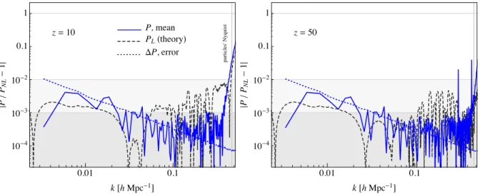
Figure 7. Absolute value of the relative difference between the mean power spectrum measured in 1000 ZA realizations (on a FFT grid of linear size NG= 480,
blue curves) and the non-linear prediction of equation (48). Also shown is the error on the mean (blue, dotted curves) and the linear prediction (black, dashed curves). Left-hand panel assumes redshift z = 10, right-hand panel z = 50. The vertical lines mark the Nyquist frequency of the ZA realizations, beyond which we expect discreteness corrections to be relevant.
We run 1000 realizations of the ZA with 3603particles in a box
of side L = 2400 h−1Mpc, at redshifts z = 10 and 50. Fig.7shows
the absolute value of the relative difference between the mean of the measured power spectra (on an FFT grid of linear size NG= 480,
blue curve) and the non-linear prediction. Also shown is the linear prediction (black, continuous curve) and the error on the mean (blue, dotted curve). One can notice that our measurements, done with PCS interpolation and interlacing, show the expected agreement with the non-linear prediction while departing from the linear one despite the very small difference (of the order of 0.1 per cent) between the two. Note that we do not subtract any shot-noise component in this case: the ZA displacements at high redshift are very small w.r.t. the initial interparticle distance defined by the grid and no significant shell-crossing occurs at small scales. The plots are limited by the particle’s Nyquist frequency, that is the Nyquist frequency of the initial ZA grid, which has a smaller value than Nyquist frequency of the FFT grid. In fact, one can notice that some additional component to the measured power spectrum appears near the particle’s Nyquist
frequency, shown in the plots by a vertical line. This is likely due to the discrete nature of the ZA realizations and therefore arising from the interplay between the FFT grid size and the particle grid (see Gabrielli2004; Colombi et al.2009, for a theoretical description of these effects). We did not attempt to derive analytically the expected correction, but we compared the results obtained from realizations characterized by a different number of particles (3603and 4003, not
shown) keeping all other variables unchanged. We did notice that the additional component near the Nyquist frequency is different for the two distributions and it is actually reduced for the one with the largest particle density.
3.4 Comparison toPOWMES
ThePOWMEScode (Colombi et al.2009), based on a Fourier–Taylor
expansion allows for a determination of the power spectrum with arbitrary accuracy at the expenses of numerical resources. In prac-tice, it reduces the contribution of aliasing by increasing the order
at SISSA on October 12, 2016
http://mnras.oxfordjournals.org/
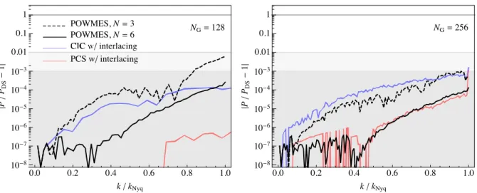
Figure 8. Relative difference between thePOWMES(black curves) measurements and our measurements (blue and red curves) with the direct summation result
performed over the N-body simulation described in Section 3.2. Dashed and continuous black curves assume, respectively, the order N = 3 and 6 in the Taylor expansion ofPOWMES. Blue and red continuous curves correspond, respectively, to the CIC and PCS interpolation schemes, both with interlacing. The left-hand
panel assumes a grid of size NG= 128, while the right-hand panel assumes NG= 256.
Nof the expansion, while providing an estimate of the residuals at each order. However, it thus requires a number of FFTs at each order given by NFFT= (N + 3)!/(N! 3!), so that the total computational
cost is O(NFFT× NG3ln NG), where NGis the linear size of the grid.
Fig.8shows a comparison between measurements of thePOWMES
code and CIC and PCS interpolation with the interlacing scheme proposed in this paper, in terms of their relative difference with the direct summation measurement of the power spectrum. For the particle distribution, we assume again the test N-body simulation of Colombi et al. (2009).
Within thePOWMESresults themselves, one can notice a clear
im-provement when comparing different orders in the Fourier–Taylor expansion (for a given grid size). This comes, however at a large computational cost. In this example, the expansion orders N = 3 and 6 forPOWMEScorrespond to a number of FFTs of NFFT= 20 and 84.
Remarkably, a comparable improvement (or better, depending on NG) can be achieved moving from CIC to PCS interpolation while
performing interlacing. In this case, we only require two FFTs.
4 H I G H E R O R D E R C O R R E L AT I O N S
A positive aspect of correcting for aliasing at the level of the density field itself consists in extending its benefits to the estimation of all higher order correlation functions, not just to power spectrum mea-surements. In this section, we consider the case of the bispectrum, i.e. the three-point function in Fourier space.
A general expression for the estimator of the bispectrum function of a triplet of wavenumbers k1, k2and k3in the case of a simple
geometry is given by ˆB(k1, k2, k3) ≡ 1 VB ! k1 d3 q1 ! k2 d3 q2 ! k3 d3 q3δD(q123) × δq1δq2δq3, (49)
where the integrals are assumed to be over a spherical shell of size &k, with radius centred at qi= ki, that is
! k d3 q≡ ! k+&k/2 k−&/2 dq q2! d*, (50)
and where the normalization factor VB, given by VB(k1, k2, k3) ≡ ! k1 d3 q1 ! k2 d3 q2 ! k3 d3 q3δD(q123), (51)
is proportional to the number of fundamental triplets q1, q2and q3
that can be found in the triangle bin defined by the wavenumbers k1,
k2and k3, with width &k. In both the integrals of equation (49) and
equation (51), the Dirac delta ensures that the triplet of qiactually
forms a closed triangle.
4.1 A fast bispectrum estimator
The implementation of the expression in equation (49) can take advantage of the integral representation of the Dirac delta, so that (see Scoccimarro2015, for extensions to redshift-space)
ˆB(k1, k2, k3) = 1 VB ! d3x (2π)3 ! k1 d3q 1 ! k2 d3q 2 ! k3 d3q 3 ×δq1δq2δq3e iq123·x = 1 VB ! d3x (2π)3 3 9 i=1 Iki(x), (52)
where the integrals Ik(x) ≡
!
k
d3q δ
qeiq·x, (53)
whose number is equal to the number Nkof k-bins we are interested in, can be evaluated as FFTs (scaling as N3
Gln NG3) and stored
in memory. The final integral in equation (52) corresponds to an O(NG3) process. The normalization factor VB(k1, k2, k3) can also be
evaluated in a similar way.
Notice that because of the exponential eiq123·xin equation (52),
this estimator cannot be applied to all values of kiup to the Nyquist frequency of the box. In fact, for a translation of the wavenumbers q given (in one dimension) by qi→ qi+2Lπ
NG
3 where NGis the grid
size and L the linear size of the box, we have q123→ q123+2πLNG
and with x = m L/NGthe exponential factor would be invariant. It
follows that the largest value for the wavenumbers k turns out to be kmax= kfNG/3, kfbeing the fundamental frequency rather than
at SISSA on October 12, 2016
http://mnras.oxfordjournals.org/
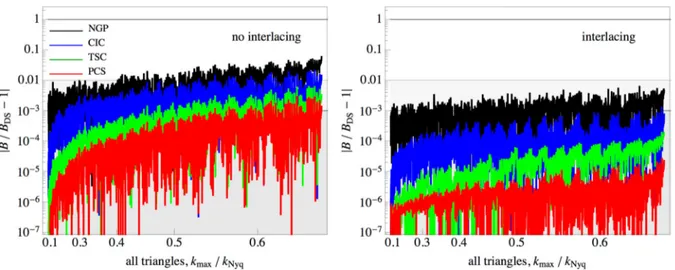
Figure 9. Aliasing effects on the bispectrum. Both panels show the relative difference between the bispectrum measured with distinct interpolation schemes
(NGP, CIC, TSC, and PCS, as black, blue, green and red curves, or different shades top to bottom) with respect to the bispectrum measured from the density field estimated by direct summation. Results on the left-hand panel do not implement interlacing, while the results on the right-hand panel do. We show all triangular configurations with triplets (k1, k2, k3) measured in units of the fundamental frequency, kf, up to 2kNyq/3 (see the text for explanation). On the x-axis
are shown the values of kmax≡ max (k1, k2, k3) in units of the Nyquist frequency.
kmax= kfNG/2, the Nyquist, as it is the case for the power spectrum
estimator.
This implementation of this estimator has been considered already in the past in the context of the large-scale structure (Scoccimarro2000; Feldman et al.2001; Scoccimarro et al.2001). Note that the expression in equation (52) is analogous to the estima-tor of the microwave anisotropy bispectrum considered by Komatsu et al. (2002).
4.2 Aliasing contributions on the bispectrum
Despite the efficient bispectrum estimator described above, it is still crucial to limit as much as possible numerical requirements starting with the size of the FFT grid. This is true, in particular, regarding the memory requirement since the implementation of equation (52) benefits from storing in memory the integrals of equation (53), i.e. a number of arrays of size N3
Gequal to the number of k-bins requested.
The interlacing scheme described in the previous section therefore results is particularly useful since it allows us to efficiently use the NG3 FFT grid, with the aliasing contribution under control all the way up to the Nyquist frequency.
Fig.9shows the relative difference between the measurements of the matter bispectrum obtained from the density interpolated on a grid to the measurements of the same quantity obtained from the density evaluated by direct summation. We assume here the 1283particle N-body simulation already considered for the power
spectrum tests. All measured triangular configurations are shown, ordered by increasing values of k1≥ k2≥ k3, k1therefore
represent-ing the largest value of the triplet. For the reason discussed above, the largest value accessible by the estimator is k = 2 kNyq/3. The
left-hand panel compares different interpolation schemes without aliasing corrections, while the right-hand panel shows the same re-sults including interlacing. In the latter case, already for the CIC scheme, the aliasing contribution is kept below the 0.1 per cent level, while 0.001 per cent is achieved with PCS interpolation. If no alias-ing correction is implemented the error can reach the few per cent level already at k ∼ 0.5 kNyq.
Not surprisingly, these results are largely consistent with those obtained for the power spectrum.
5 C O N C L U S I O N S
Standard FFT-based, power spectrum estimators routinely em-ployed in the analysis of redshift surveys data sets as well as N-body simulations, suffer from spurious contributions due to aliasing. This well-known problem is often circumvented by limiting the range of scales (wavenumbers) over which the desired accuracy could be achieved. The drawback, clearly, is the inefficient use of numerical resources as this approach clearly requires larger FFT grids than naively expected. This becomes even more problematic for higher order correlations.
Aliasing takes the form of a sum over images, each of them cor-responding to the Fourier content displaced by increasing multiples of the sampling frequency of the grid. The strength of the alias-ing contributions depends on both the interpolation kernel that goes from objects to density perturbations on the grid and the small-scale modes not supported by the grid. We quantified the systematic error on the power spectrum estimation due to aliasing in two particle distributions relevant for large-scale structure studies: an N-body simulation describing the (non-linear) matter field at z = 0 and the distribution obtained by particles displaced from a regular grid according to the ZA at z = 10, 50.
By comparing our results to the (aliasing-free) estimation by di-rect summation, we showed that in the N-body example the resulting error on the power spectrum estimation can be larger than 1 per cent already at scales roughly above half the Nyquist frequency of the grid when using the standard CIC interpolation. If the required ac-curacy is below the 0.1 per cent level, a reasonable requirement for cosmological applications aimed at the detection of small effects possibly due to non-standard physics, the usable range of scales be-comes as restrictive as k! 0.4kNyq. The problem is even more severe
when a distribution like the one obtained by ZA at large redshift is considered: in this case an accuracy of 1 per cent (0.1 per cent) is only achieved for wavenumbers k! 0.3 (0.2) kNyq.
at SISSA on October 12, 2016
http://mnras.oxfordjournals.org/
We then revisited a method to reduce the aliasing contribution based on an interlacing technique (see e.g. Hockney & Eastwood 1981; Couchman1991). We showed that using two interlaced grids removes odd images, which include the dominant contribution to aliasing. We demonstrated that this technique is able to reduce the aliasing contribution below the 0.1 per cent level for practically all wavenumbers, all the way to the Nyquist frequency of the grid, when combined with interpolations schemes of order higher than the CIC. This is true for both the examples mentioned above as well as for a comparison of the mean power spectrum measured from 1000 ZA realizations with the exact theoretical prediction. For the interpolation schemes, we considered the third-order TSC scheme and the fourth-order PCS, which are increasingly smooth schemes constructed by convolving a top-hat function with itself an increasing number of times.
While higher order schemes have the disadvantage of an in-creased time required to perform the particle assignment (without affecting the necessary memory), the payout in terms of systematic errors in Fourier coefficients can be substantial. At a fixed required systematic error, the algorithm proposed here can actually be more efficient than the standard CIC method. To make systematics in the power spectrum negligible, e.g. 0.01 per cent, one requires from CIC a grid size five times larger in each dimension than PCS with interlacing, which results in eight times more computational cost (and 62 times more memory). Similarly due to the increase in grid size, the FFT step is correspondingly slower in the CIC case.
We remark that the aliasing correction implemented via inter-lacing is performed on the density field itself and have shown that combining PCS with interlacing gives very accurate Fourier ampli-tudes and phases of density perturbations compared to the standard CIC method. It therefore improves the estimation of the power spectrum as well as any higher order correlation functions evalu-ated from such density. We showed that this is indeed the case for the bispectrum, by performing comparison to the direct summation results, as done for the power spectrum. Other approaches to limit aliasing effects in the estimation of the power spectrum as the one proposed by Jing (2005) cannot be easily extended to higher order correlation functions.
We believe that the method presented here represent a numer-ically efficient way to reduce aliasing effects in the measurement of correlation functions of particle distributions in Fourier space, relevant in a variety of cosmological investigations. A code imple-menting the algorithms here described will be soon made public. AC K N OW L E D G E M E N T S
We thank the referee, St´ephane Colombi, for making thePOWMES
code public and for useful comments and suggestions that improved
the presentation. ES thanks Julien Bel for many discussions and the NYU Dept. of Physics and the Institut des Ci`encies de l’Espai for hospitality during the completion of this project. MC has been partially funded by AYA2013-44327 and acknowledges support from the Ramon y Cajal MICINN programme. RS was partially supported by NSF grant AST-1109432, and HMPC was supported by NSERC.
R E F E R E N C E S
Bond J. R., Couchman H. M. P., 1988, in Thorne K. S., ed., Proceedings of the 2nd Canadian Conference on General Relativity and Relativistic As-trophysics, wgg(θ) as a Probe of Large-Scale Structure. World Scientific
Publishing Company, p. 385
Chaniotis A. K., Poulikakos D., 2004, J. Comput. Phys., 197, 253 Colombi S., Jaffe A., Novikov D., Pichon C., 2009, MNRAS, 393, 511 Couchman H. M. P., 1991, ApJ, 368, L23
Couchman H. M. P., 1999, in Miyama S. M., Tomisaka K., Hanawa T., eds, Astrophysics and Space Science Library, Vol. 240, Numerical Astro-physics. Kluwer, Dordrecht, p. 1
Cui W., Liu L., Yang X., Wang Y., Feng L., Springel V., 2008, ApJ, 687, 738
Feldman H. A., Frieman J. A., Fry J. N., Scoccimarro R., 2001, Phys. Rev. Lett., 86, 1434
Gabrielli A., 2004, Phys. Rev. E, 70, 066131
Haugbølle T., Frederiksen J. T., Nordlund A., 2013, Phys. Plasmas, 20, 062904
Hockney R. W., Eastwood J. W., 1981, Computer Simulation Using Particles. McGraw-Hill, New York
Jasche J., Kitaura F. S., Ensslin T. A., 2009, preprint (arXiv:0901.3043) Jing Y. P., 2005, ApJ, 620, 559
Komatsu E., Wandelt B. D., Spergel D. N., Banday A. J., Gorski K. M., 2002, ApJ, 566, 19
Laureijs R. et al., 2011, preprint (arXiv:1110.3193) Levi M. et al., 2013, preprint (arXiv:1308.0847)
Peebles P. J. E., 1980, The Large-Scale Structure of the Universe. Princeton Univ. Press, Princeton, NJ
Schneider P., Bartelmann M., 1995, MNRAS, 273, 475 Scoccimarro R., 2000, ApJ, 544, 597
Scoccimarro R., 2015, Phys. Rev. D, 92, 083532
Scoccimarro R., Feldman H. A., Fry J. N., Frieman J. A., 2001, ApJ, 546, 652
Taylor A. N., Hamilton A. J. S., 1996, MNRAS, 282, 767
Yang Y.-B., Feng L.-L., Pan J., Yang X.-H., 2009, Res. Astron. Astrophys., 9, 227
This paper has been typeset from a TEX/LATEX file prepared by the author.
at SISSA on October 12, 2016
http://mnras.oxfordjournals.org/
![Figure 4. Same as Fig. 3 , but comparing the phases of the Fourier-space mode, φ = arctan [Im δ(k) / Re δ(k)].](https://thumb-eu.123doks.com/thumbv2/123dokorg/8094249.124719/9.892.150.744.82.661/figure-fig-comparing-phases-fourier-space-mode-arctan.webp)