Alma Mater Studiorum – Università di Bologna
DOTTORATO DI RICERCA IN
METODOLOGIA STATISTICA PER LA RICERCA
SCIENTIFICA
Ciclo _XXIV__
SETTORE CONCORSUALE DI AFFERENZA: 13/D3- DEMOGRAFIA E STATISTICA SOCIALE SETTORE SCIENTIFICO-DISCIPLINARE:SECS-S/04 – DEMOGRAFIA
TITOLO TESI
Parameter estimation in a growth model for a
biological population
Presentata da: Elettra Pignotti
Coordinatore Dottorato
Relatore
PROF. ANGELA MONTANARI
PROF. DANIELA COCCHI
Correlatore
Introduction
4
1 The growth curves in Biology
7
1.1 Growth Curve Model
7
1.1.1 Bell-shaped curve
8
1.1.2 Unbounded growth
9
1.1.3 Bounded growth
9
2 The use of the von Bertalanffy curve to estimate the solitary coral growth
13
2.1 Coral growth and problems of its modelling
13
2.2 The von Bertalanffy growth function for solitary corals
15
2.3 The methods used in marine biology for estimating the von Bertalanffy growth parameters
18
2.3.1 The Gulland-and-Holt (GH) plot
18
2.3.2 The size-increment method proposed by Fabens
19
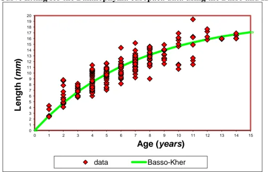
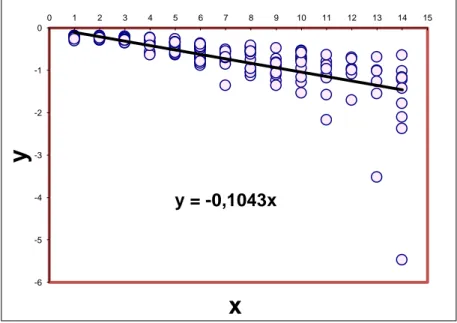
2.3.3 The linearization proposed by Basso and Kehr
19
2.4 Gallucci and Quinn parameterization
20
2.5 A new proposal of parameterization based on Gallucci and Quinn model
20
3 An alternative approach to estimate the growth curves: hierarchical models
22
3.1 The hierarchical approach
22
3.2 Basic nonlinear regression model
24
3.3 Newton’s method for nonlinear function estimation
26
3.4 The hierarchical model specification proposed by Lindstrom and Bates
27
3.4.1 Intra-site variation
28
3.4.2 Inter-site variation
29
3.5 Hierarchical nonlinear model for the solitary corals
30
3.5.1 The standard parameterization
30
3.5.2 The new proposed parameterization
33
4 Growth curves for corals
35
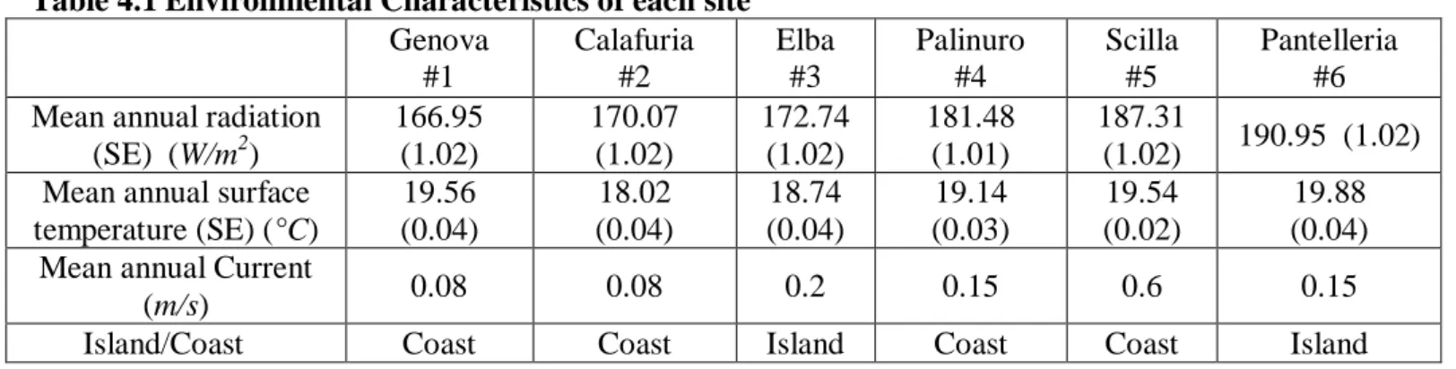
4.1 The Solitary Corals of our study
35
4.1.1 Balanophyllia europaea and Leptopsammia pruvoti
35
4.3 Explorative analysis
38
4.3.1 Balanophyllia europaea
38
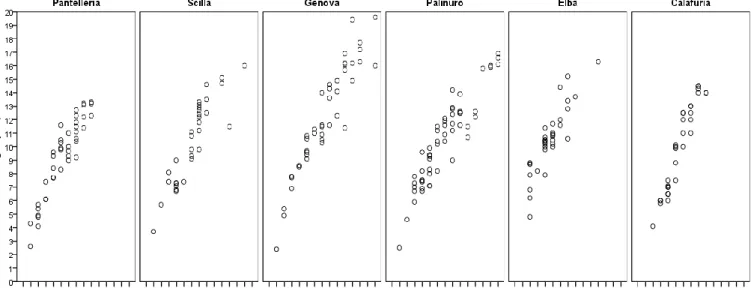
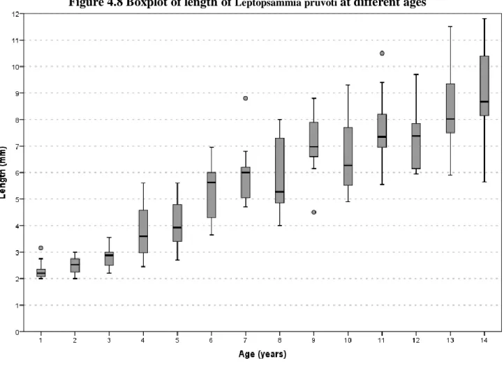
4.3.2 Leptopsammia pruvoti
40
5 Results with the traditional Methods used in marine biology for the
Von Bertalanffy Growth Function fitting
42
5.1 The Gulland-and-Holt (GH) plot
42
5.2 The size-increment method proposed by Fabens
47
5.3 The linearization proposed by Basso and Kehr
51
5.4 Newton’s method for nonlinear function estimation
57
5.4.1 The standard parameterization
57
5.4.2 The new parameterization
59
5.5 Results with nonlinear hierarchical model
62
5.5.1 The method giving the best fit for the Balanophyllia Europaea
64
5.5.2 The method giving the best fit for Leptopsammia Pruvoti71
6 Conclusions
77
Bibliography
79
Introduction
Marine organism growth has been the focus of increasing interest, over recent years, among marine biologists (Stolarski et al., 2007), (Goffredo et al., 2000). The goal of this work is therefore the problem of estimating the growth of some very common marine organisms in the Mediterranean sea, belonging to the family of corals, better known as solitary corals. Little is known about their growth mechanism and the influence of environmental factors. Furthermore the coral reproductive ability depends on how fast they reach the minimum size for reproduction.
The individual age of these corals may be estimated through their body size: standard age-based growth and population dynamics models may be subsequently applied. Demographic parameters highlight relationships between organisms and their environment, and contribute to the assessment of habitat stability; in addition, information on population turnover may contribute to techniques for the restoration of damaged or degraded coastal areas.
Due to difficulties and costs of recording the ages of corals, it is necessary to build up reliable growth models to infer coral age from their body size. In fact corals have a truncated cone geometry and their growth is isometric. Since growth depends on annual rings of calcium carbonate in coral bodies, the coral body size is directly related to the coral age and the ring thickness, which is in turn related to genetic and environmental factors. As a consequence, coral growth can be described as a function of several parameters, having a biological meaning, linked to age by a non-linear relationship.
In biology, the estimates of such parameters are generally obtained by using different strategies of linearization (see for instance Gulland and Holt ,1959; Fabenas,1965; Basso and Kehr,1991).
Biologists follow two main strategies for collecting data useful to estimate these parameters and consequently the coral growth.
In the first one the sample consists of corals randomly chosen in the site under study; each coral is measured repeatedly at fixed intervals of times in situ; the results are the mm/months of growth of each coral; then the parameters describing individual growth are estimated by a suitable method. Finally, the parameters for the
population are subsequently estimated starting from the individual ones and a growth curve for the population is finally constructed (Harper, 1977; Grigg et al. ,1984; Ross et al, 1988; Goffredo. et al., 2000). In the second approach, the sample consists of colony of corals. Corals of different sizes of each colony are random collected, measured and dated. Each coral is measured only once because collection and dating causes the destruction of the coral. The growth curve for each colony is constructed using the dimensions of the body size of corals at different ages. The parameters of the growth curve for the population are then estimated by the parameters of the growth curve for each colony (Goffredo et al., 2000; Epstein et al. 2001; Goffredo and Chadwick-Furman, 2003;Goffredo and Lasker, 2008).
Apart from the method used for collecting data, the estimate of the growth curve parameters is traditionally is traditionally obtained by linear models that simplify non–linear relationships. The influence of environmental factors is accounted for by their linear correlation coefficient with the parameters (McClanahan, 2009; Goffredo and Caroselli, 2010; Harrell Yee and Barron, 2009; Soto et al., 2011). For example, Goffredo and Caroselli (2010) assessed the influence of the sea surface temperature (SST) on coral growth by finding a linear correlation between SST and estimated growth parameters in colonies located in places having different SST.
The above approaches share two main drawbacks: first, linearization is introduced regardless the behaviour of observed data, without considering the presence of variability in the body size of corals of the same age. This could cause an error in the parameter estimates. Furthermore no connection is hypothesised between the parameter estimate error at the coral (or colony) level, the parameter estimate error at the population level and the error of the linear regression between the parameter and the environmental factors.
For these reasons we propose instead a non-linear mixed effect model with the aim to overcome all these limits related to the estimation of coral growth and to obtain more reliable parameter estimates of the population growth curve, in this case avoiding forced linearization.
In addition, a new parameterization of the coral growth curve is proposed in order to identify parameters that are sensitive to the environment from those depending only on the genetics of the coral.
traditional methods used to estimate the parameters of the curve; in the chapter there is also the description of a new proposed parameterization for the curve. Chapter 3 describes the new approach using a hierarchical nonlinear model is performed, whereas chapter 4 describes the data sets and the models using both parameterizations of the growth curve. Chapter 5 shows the results of the traditional linearization methods used in biology to estimate parameters; furthermore an estimate of the parameters using a nonlinear regression is proposed. Chapter 5 presents the results for the nonlinear hierarchical model applied to both parameterizations with and without considering the influences of environmental covariates.
1 The growth curves in Biology
1.1 The Growth Curve Model
Growth curve models are used to describe how a particular quantity increases or evolves over time and consists of a sequence of data points taken at successive moments in time commonly spaced at uniform intervals. These models are also used to identify the type of growth pattern of different populations and to study the related variables in different fields of applications, for examples biology, ecology, demography, population dynamics, finance, econometrics, where a lot of models are developed including: mechanistic models, time series models, stochastic differential equations, etc.
In biology, growth is considered to be both related to the physical dimension and to the population of an organism; it is considered to be a fundamental property of biological systems studied at the colony level (group level), as well as for each organism (individual level). Growth curve models are based on longitudinal data, so measurements are repeatedly taken on a response variable at different time points. Different kinds of growth patterns have been used in the literature to model the various types of realistic growth mechanisms. The first study pertaining to growth curves was presented by Wishart (1938) and differences between growth curves were discussed by Burnaby (1966). A wide and organic discussion of growth curve models (GCM) was introduced by Potthoff and Roy (1964) and subsequently expanded among others by Rao (1965). Results lead to summarizing growth curve shapes into three different growth mode categories: unbounded, bounded and bell-shaped curves (Figure 1.1). They behave similarly in early times because the energy available is all used for t growth, then saturation starts to play a significant role. In fact saturation is due to an increasing part of energy used to maintain the reached dimension and this process can be very different among organisms. In bell-shaped curves, the increase eventually turns into decrease after passing through a peak point: bell-shaped curves can be symmetric or asymmetric. However, the curves displayed in Figure 1.1 have to be considered as examples, and there are a multitude of mathematical functions available for each type of growth mode (Höök et al., 2011).
Figure 1.1 general growth modes
1.1.1 Bell-shaped growth
Bell-shaped growth (Hubbert, 1956) includes a portion of time with a positive slope, an inflection point which becomes also a maximum and finally a portion of time with a negative slope. Bell-shaped curves have many different shapes and may be symmetric or asymmetric. They are often closely related to sigmoid
functions and commonly appear as their derivatives (Höök et al., 2011). These curves have frequently been
used in a wide array of disciplines, but initially were developed to describe and predict production growth in biological systems (cell production) or in bioenergetics systems (fuel production). Hubbert (1956) was among the first to formulate a basis for the extrapolation of finite resource production curves into the future and bell-shaped growth curves were an important cornerstone in such framework. He assumed that production levels begin at zero, before production has started, and end at zero, when the resource has been fully exhausted. In between, production would pass through one or several maxima. Conceptually, all resources are subjected to a physical limitation, due to the earth’s intrinsic finiteness. Such physical resource limitations affect the general growth pattern. The limitation lies primarily in the maximum cumulative production that can be reached. So after an initial increase the production reaches a maximum, then slows down towards zero because of the finiteness of the resource. In biology they were developed to describe and
predict growth in biological systems such as in organs of the human body that show degeneration or involution: a typical example is the human brain which grows fast in children and slowly in adults; it reaches its maximum development in adult age and then shrinks slowly until old age when shrinking occurs rapidly.
1.1.2 Unbounded growth
All forms of unbounded growth, regardless of their mathematical nature, are clearly not suitable in the long-term. Linear growth is obviously slower than exponential growth but in the long run all unbounded growths tend towards infinity (Höök et al., 2011). Growth in economic theory is the most commonly used unbounded model; in fact, growth is believed to continue forever, but these models can be interesting only if they are studied over a “short” time (Bartlett, 1993 1999 and 2004) because models change according to different economic conditions. Unbounded growth is supported by those who believe that the obvious physical limitations of the earth do not necessarily imply an economic limitation (Simon, 1981); in fact conditions for the economic growth are continuously changing so when a source of economic growth is ending it is replaced by another one brought about by new technology or inventions or different behavioural patterns of humans. Others believe that that natural resources are not needed for economic growth (Solow, 1974) or even that human ingenuity can act as a powerful force capable of overcoming all possible physical limitations (Radetzki, 2007).
1.1.3 Bounded growth
This growth model is subject to physical limitations that affect growth rates, making growth slow down over time and asymptotically strive towards a maximum value (Janoschek, 1957; Beverton and Holt, 1957). Bounded growth occurs in many cases, such as human growth, organ growth, population growth and finite resource production. Growth may actually continue indefinitely but the rate of growth approaches zero as time tends to infinity. This is well known in many biological systems where an organism may grow quickly in its juvenile stage but then its growth slows down as it reaches maturity. The limiting factor lies rather in
resources left for further growth. In the biological sciences, this condition is often modelled as proportionality between growth rate and actual size.
Sometimes these growth curves imply a rapid growth in the beginning, which later slows down; as in the case of exponential growth curves they are commonly used to estimate the length of some organisms, or the size of the skull and the brain.
Some curves have an inflection point (flex): the initial increase is slow therefore the first part of the curve appears flat; then growth increases rapidly so the curve turns upwards sharply until a second slow increase occurs, thus giving the curve a flat appearance again. An example can be found in sigmoid growth curves where growth is slow at the beginning of the time of observation and at the end but faster in the central time of observation.
The weight and volume of the body and of most organs show a sigmoid growth pattern initially, since the rate of growth in mass is low but increasing. The growth rate reaches a maximum, which corresponds to the inflection point in the curve, and then slowly declines to zero when the organism achieve their mature weight.
Richards (1959) proposed a sigmoid function developed as a generalization of classical growth curves and shown in Figure 1.2. This function is characterised by four parameters not very easy to interpret in many applications. Moreover it converges less frequently than the curves that we describe in what follows, especially if data do not already include the inflection point. It is actually used to fit data on forest growth.
Figure 1.2 Richards curve
The function is
1 kt M y t L ( be ) 1.1 0 2 4 6 8 10 12 14 16 18 0 10 20 30 40where y(t) is the dimension, L∞ is the asymptotic maximum, b depends on the difference between the
asymptotic maximum ant the initial dimension y(0), k is the growth rate and M shapes the way the asymptotic maximum is reached and the position of the inflection point.
Other well-known sigmoid curves are the Gompertz curve (Gompertz, 1825), the logistic curve (Verhulst, 1838) and the von Bertalanffy curve (von Bertalanffy, 1938).
The Gompertz curve (Gompertz, 1825) is shown in Figure 1.3, and was developed for the calculation of mortality rates. It is one of the most commonly used curves in growth mathematics and it is characterized by slow growth at the beginning and the end.
Figure 1.3 Gompertz curve
The function is
be-kty t L ( e ) 1.2
where y(t) is the dimension, L∞ is the asymptotic maximum, b sets the displacement along the abscissa and k
is the growth rate.
The Logistic curve, shown in Figure 1,4, was developed by Verhulst (1838) as a model for populat ion growth. It is characterized by an inflection point independent of measurements so it is often used for sigmoid growth where the inflection corresponds approximately to one-half of final size.
0 2 4 6 8 10 12 14 16 18 0 5 10 15 20 25 30 35 40
Figure 1.4 Logistic curve The function is 1 kt L y( t ) ( be ) 1.3
where y(t) is the dimension, L∞ is the asymptotic maximum, b sets the displacement of the inflection point
and k is the growth rate.
The von Bertalanffy curve is a bounded growth curve, derived from the von Bertalanffy Growth Law (1938) and based on the balance by the energy income provided by “food” and the fraction of this energy used for growth. The most common parameterisation of the von Bertalanffy Growth Law was described by Beverton and Holt (1957) and consists of a Richards model with the M shape parameter equal to 1. In this curve, dimension is a non-linear function of time based on 3 parameters, each with a physical meaning: maximum dimension, growth rate, and time at which the coral size is equal to zero. Their role and importance are discussed widely in the next chapter.
0 2 4 6 8 10 12 14 16 18 0 10 20 30 40
2.
The use of the von Bertalanffy curve to estimate the solitary coral
growth
2.1 Coral growth and problems of its modelling
Most simple marine organism populations are analysed considering individual body size. This measure is fundamental, since all physiological processes are related to size, including rates of metabolism, foraging and digestion (Peters, 1983; Calder, 1984). Body size is directly linked to life-history traits and individual competitive ability (Fox, 1975; Arendt, 2007). For these reasons, a reliable estimate of the growth parameters for a population of a certain area is important. In particular, the body size o f corals is strictly related to the reproductive activity because size has to be big enough to let the planulae get out of the oral disk; where corals reaching the dimension of reproduction in early ages have more reproductive success. Growth modelling and the analysis of intra-population patterns of body size variability over time are the central topics in animal population biology, since the internal size structure of populations may have a decisive influence on the population dynamics (De Angelis et al., 1993; Imsland et al., 1998; Uchmanski, 2000; Kendall and Fox, 2002; Fujiwara et al., 2004).
De Angelis et al. (1993) observed that model structure and parameter values are based on observations of individuals, so the natural variation among individuals and the stochastic nature of their fates should be incorporated in any model used. In this framework, the numbers of individuals necessary for estimation needs to be high. This model produces a reliable estimate of the population response to environmental variation only if data come from well-documented long-term studies of individuals belonging to the same populations. Imsland et al. (1998), Kendall and Fox (2002) and Fujiwara et al. (2004) underline that a model should incorporate population-specific data on ecological energetics, thermal and size dependence of digestive physiology and metabolic rates, energetics of individual growth, allometric relationships, social structure and mating system, and the dependence of mortality rates on age, size, and social status of individuals. This means that individual-level processes are determined by the organism’s physiological state and interactions with its environment, whereas the population state is the distribution of individuals over all
In general, the von Bertalanffy growth function (VBGF, von Bertalanffy, 1938) is the most widely accepted relationship to describe the growth of fish and other marine organisms (Ricker, 1979; Cailliet et al., 2006). The VBGF describes the relationship between age and mean length of a population, whereas the variability among individuals of the same age (e.g. the variance or even the distribution of each cohort) is not included. Each individual is born with a specific genetic constitution that, to a certain extent, controls its growth profile (Sainsbury, 1980), but many physical and biological factors, such as water temperature (Sumpter, 1992), dissolved oxygen (Brett, 1979), photoperiod (Imsland et al., 2002), and the availability and type of food sources (Rilling and Houde, 1999) affect the actual growth rates achieved. In addition, the plasticity of phenotypes has been shown to be adaptive across environmental gradients (Conover and Munch, 2002; Ernande et al., 2004). Therefore, a suitable growth model should take into account individual and environmental variability.
In both ecological (Arino et al., 2004) and evolutionary (Conover and Munch, 2002; Ernande et al., 2004) contexts, one of the challenges of researchers is to model how the body size o f an individual changes over time and to understand from the growth model what kind of probability distribution is suitable for the size of an individual as age increases (Lv and Pitchford, 2007; Fujiwara et al., 2004). In corals, as in other animals, the first source of variability is rooted in physiological processes and is the net result of two opposing processes, catabolism and anabolism (von Bertalanffy, 1938). The inter-individual variability in growth is the result of several internal (genetic) and external (environmental) factors, which affect these physiological processes. Pilling et al. (2002) and Clarke et al. (2011) state that the estimate of the growth curve of a population in each collection site is better performed by the growth model proposed for the size-at-collection data than a repeated measure model on a sample of individuals; in fact a single observation per individual better describes the mean growth parameters.
In fact, whilst each individual is born with a personal genetic architecture, which primarily determines its growth profile, a number of physical and biological factors, such as water temperature, solar radiation, the availability of appropriate food sources etc, have been shown to affect growth rates.
Differences in size among individuals that are established early in their life history can persist or be amplified (Ricker, 1958) if growth is positively size dependent and if there are positive correlations in
growth over time among individuals. The latter phenomenon is referred to as ‘growth autocorrelation’ (Pfister and Stevens, 2002) and is the reason for persistent growth differences among individuals. Similarly, differences among individuals in size can dampen over time (Ricker, 1958) if growth is negatively related or unrelated to size and there is no growth autocorrelation among individuals. The pattern of growth autocorrelation may be the result of several mechanisms, including factors that are intrinsic to the organisms, such as genetic or behavioural traits that confer performance differences among individuals (see Fraser et al. 2001). Alternatively, factors extrinsic to organisms, such as environmental heterogeneity, can cause persistent differences among individuals.
In conclusion, the underlying sources of growth variability in a population cannot generally be known. For size-at-collection data the consequences of not accounting for individual growth variability, or assuming the wrong source of variability, are less with respect to tag–recollection data, even when individual variability is high or data coverage is poor. So to reach a reliable size-at-age estimation the best way is to estimate VBGF parameters under a stochastic model using size-at-collection data.
2.2 The von Bertalanffy growth function for solitary corals
The main approach followed by biologists to obtain insights into metabolic phenomena is the study of the metabolism as a balance of energies: the energy entering the organism from food, heat, radiation and the energy necessary for feeding, growth, reproduction, maturation and maintenance. The mechanisms that are responsible for the organization of metabolism are not species specific (Kooijman, 2000). This care for generality is supported both by the universality of physics and evolution and the existence of widespread biological empirical patterns among organisms. In particular the growth of isomorphic organisms with abundant food is well described by the von Bertalanffy growth curve (Putter 1920; von Bertalanffy 1938). The identification of the curve is based on the physical principle that mass and energy are fixed quantities as starting points, so that the maintenance rate coefficient is the ratio between the cost of volume maintenance EM and the cost of growth EG ( M M
G
E k
E
proposition that organisms of the same species have a maximum structural length L∞. (Kleiber ,1947) All
these considerations point to von Bertalanffy’s law: the growth curve of an isomorphic juvenile or adult individual with constant food availability or abundant food is then
dL
k( L L )
dt 2.1
The von Bertalanffy growth rate k is given by
1 3 3 h -M ( L L ) k k 2.2
where Lh is the reduction in length due to the energy used for heating (Lh is the ratio between the cost of the
surface maintenance ES, associated mainly with heating, and the cost of volume maintenance EM) and is
the energy conductance (a measure of energy transfer efficiency).The set of parameter values is individual-specific. Individuals differ in parameter values and selection leads to evolution characterized by a change in the (mean) value of these parameters. However, it is important to underline that, in agreement with
Errore. L'origine riferimento non è stata trovata., L∞ and the growth parameter k are correlated; the von
Bertalanffy growth rate decreases, in fact, with ultimate length: different combinations of k and L∞ can give
almost the same fit to data, except when a wide range of ages is represented. Again, a high value of k combines with a low value of L∞ and vice versa (Sparre and Venema, 1992).
The von Bertalanffy’s law (Putter, 1920; von Bertalanffy, 1938) is one of the most universal biological patterns (Fraser et al., 1990; Strum, 1991; Schwartz and Hundertmark, 1993; Ferreira and Russ, 1994; Ross et al., 1995) and can be considered the pillar of the laws describing the growth of organisms. Of course complex organisms have interactions between the different parts of their body and with the environment, so the description of growth only in terms of a physical law is very difficult. For simple organisms like corals this law well describes the body growth and can be used also for organisms of the same species wit h different food availabilities. In the latter case Kooijman et al. (2007) asserts that unlike
Errore. L'origine riferimento non è stata trovata., the logarithm of the von Bertalanffy growth rate
decreases with ultimate length,
1
ln( k ) L
The most common parameterization of the solution to the differential equation 2.1 is 0
1 k( t t )
y( t )L ( e ) 2.4
where y(t) is the dimension, L∞ is the asymptotic maximum, k is the growth rate and t0 is interpreted as the
age when an individual would have been of zero length.
Biologists use the von Bertalanffy model with size at birth equal to 0 to describe solitary coral growth; when the size at birth is considered zero, thus t0=0, the curve starts from the origin, and the
Errore. L'origine riferimento non è stata trovata. becomes
1 kty t L ( be ) 2.5
From a biological point of view the VBGF has three meaningful parameters:
1. L0 is the mean length at birth (t = 0), which is species-specific and for solitary corals is universally
considered to be very close to zero
0 0 or equivalently 0 0
L t
2. L∞ is the maximum mean length achievable by the species, with set environmental conditions and food
availabilities, when t goes toward infinity.
3. k is the so-called Brody growth rate coefficient, but it is actually the exponential rate of approach to the asymptotic size, his unit is the reciprocal of the unit time (e.g. year-1).
The main problem for biologists is then a reliable estimate of these parameters; the estimate should face two basic matters: the strong correlation between the parameters and the potential influence on them of environmental covariates which shouldn’t affect, in agreement with the metabolic theory, the ultimate length L∞.
For these reasons, we propose a new parameterization able to capture the effect of environmental covariates only by one parameter, isolating the role of the ultimate length L∞ and, in addition, to propose a method to
2.3 The methods used in marine biology for estimating the von Bertalanffy
growth parameters
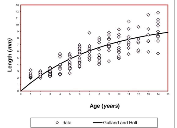
2.3.1 The Gulland-and-Holt (GH) plot
The GH plot (Gulland and Holt, 1959) is one of the most widely used methods in biology: it is based on annualized growth rates plotted vs. mean length at first and second measurements. Indeed the von Bertalanffy growth curve implies that the growth rate (dL
dt ) declines linearly with length.
This relationship between length and growth rate can be used to estimate the two parameters L∞ and k. In a
standard GH plot, the growth rate dL
dt of an experimental interval is plotted over the mean length in that
interval).The differential form is
mean mean dL L'( t ) kL kL k ( L - L ) dt 2.6
or in terms of growth increments per interval (length L1 and L2);
2 1 2 1 2 1 2 L - L L L a b t - t a a k - b L -b k 2.7
For corals the mm/year growth is calculated for each individual and then plotted against the individual length: the least squares estimation of the straight line parameters are then used to calculate L∞ and k.
This method has several limitations:
it is adequate only if the time interval Δt=t2-t1 is infinitesimal;
it should be used only with follow up measurements, it is commonly used instead also with the length-at-capture data;
it does not take into account the correlation between L∞ and k;
it is a deterministic method which does not take into account any possible statistical fluctuation and does not provide any confidence measure of the estimate.
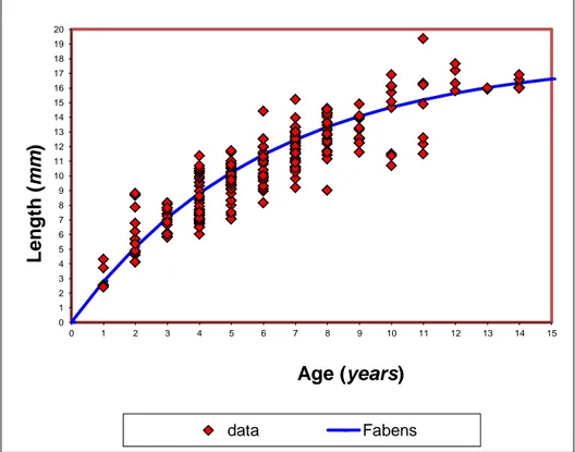
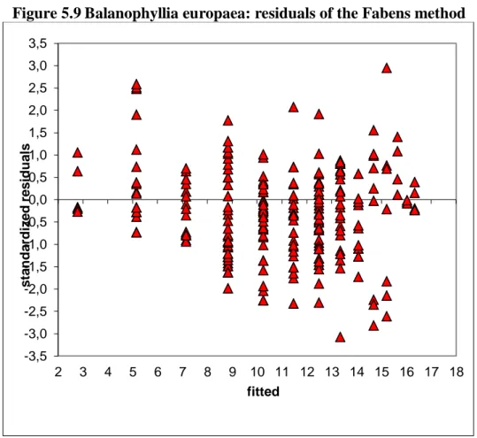
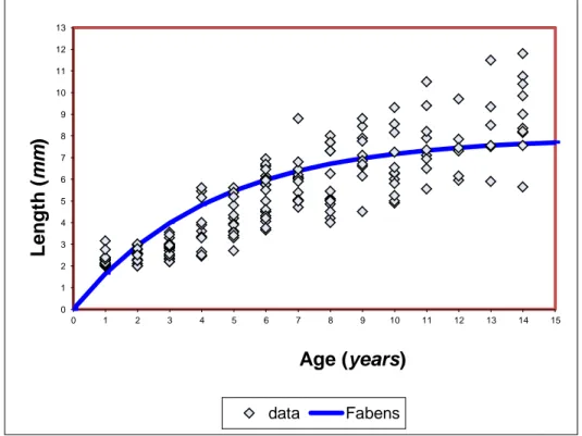
2.3.2 The size-increment method proposed by Fabens
The size-increment method proposed by Fabens (1965), fits the von Bertalanffy model by the least squares method to observed lengths, using data on known growth increments in known time intervals but making no assumption about absolute age according to:
1
k t k t
t t t
L L e L ( e ) 2.8
where Δt is the time increment between the two measured points Lt and Lt+Δt.
Indeed for corals the growth is measured for each individual at fixed intervals of time, so Δt is constant and then a linear regression of Lt+Δt against Lt will generate a slope of e k tand an intercept of L 1( e k t). This method has several limitations:
it overestimates k and underestimates L∞ .The bias appears to be associated with a failure to account
for the redistribution of the error term when the basic growth equation is transformed to eliminate the necessity of estimating age;
it does not take into account the correlation between L∞ and k;
it does not take into account the possible influence of environmental parameters;
it does not take into account the level and the distribution of the error at the individual and population of a colony level.
2.3.3 The linearization proposed by Basso and Kehr
The linearization proposed by Basso and Kehr (1991) fits the von Bertalanffy model imposing as L∞ the
largest size found in individuals of each species and then considering the linear regression between
1 Lt ln L
0 1 Lt ln - - kt kt L 2.9
The above models are stated as deterministic, while linearization is valid only considering a small neighbourhood of the studied times, so nonlinear statistical methods can definitely improve the results.
2.4 Gallucci and Quinn parameterization
Gallucci and Quinn (1979) noted that comparisons of “growth" between two or several groups should involve both k and L∞. However, because of the generally high correlation between these two parameters,
simultaneous hypothesis tests of these two parameters are non-standard and difficult to interpret. They introduced a new parameter, ω= kL∞ asserting that it is a sensible index to compare two or more growth
curves because it captures both the essential features of body-size growth. The new parameterization can be then achieved, by solving for L∞ and substituting it In Errore. L'origine riferimento non è stata trovata.,
1 kt
y( t ) e k 2.10In the same article Galucci and Quinn (1979) state that ω can be thought of as a growth rate because the units are in length-per-time, which, in fact, corresponds to the instantaneous growth rate near t=0 in the case of corals. Furthermore, they claim that ω is the appropriate parameter to use to compare populations because of its statistical robustness owing to its normality (with small variance) for different populations of the same species (Moreau et al. 1987).
2.5 A new proposal of parameterization based on Galucci and Quinn
model.
Kooijman (2000) underlines that for organisms of the same species with different food availabilities the logarithm of the von Bertalanffy growth rate decreases linearly with ultimate length as stated in
Errore. L'origine riferimento non è stata trovata. 1
ln( k ) L
So, different combinations of k and L∞ can give almost the same fit to data, except when a wide range of
ages is represented. Again, a high value of k combines with a low value of L∞ and vice versa (Sparre and
Venema, 1992)
Our proposal is then to use a different parameterization of
Errore. L'origine riferimento non è stata trovata.
1 c L te y( t ) L e 2.11 where c ln( k )L 2.12
This new approach might lead to more reliable results when including the effect of environmental covariates, in fact, as Kooijman (2008) pointed out, for simple isomorphic organisms with different food availabilities L∞ could be considered independent of external factors; so the influence of covariates x ,...x 1 v
representing environmental influences could be attributed to the new parameter
1
v
c f ( x ,..,x ) 2.13
The new parameter c could be seen then as the part of the length growth accountable to site-specific conditions such as environmental factors.
This parameterization, compared to the traditional one, has the advantage of isolating the parameter sensible to environmental influences, so that it is possible to obtain a more meaningful and parsimonious statistical model when covariates are involved. The deterministic methods used by biologists do not suit with this parameterization because they were designed to find k and L∞, while the new parameterization does not
3 An alternative approach to estimate the growth curves:
hierarchical models
3.1 The hierarchical approach
The models used by biologists are deterministic in the sense that they do not take into account differences among individuals of the same population and differences among populations related to different environmental conditions. They furthermore introduce a forced linearization which produces an unreliable estimation of the VBGF parameters; in fact the VBGF is a nonlinear relationship. A first step to improve the parameters estimation is the use of a nonlinear regression model so that it is possible to consider directly in the model the functional form linking growth and age. The nonlinear models are based therefore on assumptions often violated in the corals growth; in addition the studied data have two sources of variation: the coral population and the sites of collection. It comes natural then to get to nonlinear hierarchical models. Therefore a better approach could be a non-deterministic model in which each coral is characterized by different parameter values of the VBGF: in this way, each single coral has its own couple of parameters,
L ,k
, in the case of the classic VBGF parameterization, or
L ,c
, in the case of the new proposed VBGF parameterization, which is retained throughout its life (Sainsbury, 1980). According to biologists, the parameters values of corals collected in the same site, leaving in an environment characterised by the same sea surface temperature, sea current and solar radiation, should be more alike than those of corals collected in different sites. The parameters describing the growth of a coral can then be seen as a sum of different contributions: the species contribution common to all corals, the site contribution common to all corals exposed to the same environmental characteristic and a random contribution typical of the single coral attributable to immeasurable aspects. This approach points directly to a hierarchical model. Another critical aspect of the deterministic approach is the forced linearization; the statistical approach provides techniques to estimate the parameters while maintaining the nonlinear relationship. Combining the two aspects we come to the hierarchical nonlinear models: the coral growth curve can be then estimated via the nonlinear least squares method; where the species contribution, common to all the corals, is considered as a fixed effect; the site contribution related to all corals exposed to the same environmental characteristics isconsidered as a random effect, which might depend on environmental covariates; the random contribution typical of the single coral can be seen as the residual error.
In fact, hierarchical nonlinear models for data in the form of continuous, repeated measurements on each of a number of individuals, are a popular platform for analysis when interest focuses on individual-specific characteristics and has gained broad acceptance as a suitable framework for such problems. The central concept of hierarchical models is that certain model parameters are themselves modelled; in other words, not all the parameters are directly estimated from the data, rather some of them are calculated from estimates of the model’s hyperparameters which are in turn estimated from the data. The latter parameters are sometimes referred to as “random effects”. They are to be distinguished from “fixed effects,” which are not modelled, but are instead estimated directly from the data. A hierarchical model can have both, so it is often described as a “Mixed effects model”.
Hierarchical nonlinear models may be regarded as both an extension of the nonlinear regression models and the hierarchical linear models. A natural framework is the two-stage model that takes into consideration intra– and inter-individual variations, as in mixed effect models. Hierarchical nonlinear models can be considered mixed effect models where some, or all, of the fixed and random effects occur non-linearly in the model function. From a non-linear point of view they can be seen as nonlinear regression models for independent data (Bates and Watts, 1988) where random effects are incorporated in the coefficients to allow them to vary by group, thus inducing correlation within the groups. From a mixed effect point of view they can be seen as linear mixed effect models where the conditional expectation of the response, given the random effects, is allowed to be a nonlinear function of the coefficients.
Pinheiro and Bates (2000) discuss three important advantages of nonlinear hierarchical models:
interpretability. The modelling approach requires that one explicitly model. Judgment as well as background empirical or theoretical knowledge can be used to guide the choice of nonlinear functional form;
parsimony. A well-chosen nonlinear function can model a non-linear process with fewer parameters than a linear model with multiple polynomial terms. In addition, the hierarchical modelling approach
allows one to replace a potentially large number of subject-specific indicator variables and interaction terms with a small number of hyperparameters;
validity beyond the observed range of the data. Of course it is always dangerous to use a model to extrapolate beyond the data. However, this approach at least offers a framework within which one can harness one’s background knowledge when specifying a model. Such an approach is less likely to lead one astray than a less parsimonious or more atheoretical “curve-fitting” approach.
3.2
Basic nonlinear regression model
The nonlinear regression models are the starting point to improve the estimation of the parameter values of the VBGF. For longitudinal data the used method are mostly based on least-square, maximum-likelihood and Bayesian estimation procedures as can be seen in Gallant (1987), Seber and Wild (1989), Genning et.al (1989), Davidian and Giltinan (1995), Vonesh and Chinchilli (1997).
Let yj be the generic observation of the ith of M sites, where j=1,..,ni, the model can be written then as
,
( )
j j j
y f x 3.1
where f(.) is a nonlinear function, is the (px1) vector considering the p parameters of the functions and 𝜀j is
the random error. The function f(.) should satisfy j=f(xj,) for one value of in and for all values of x.
This condition, if verified, implies that E(𝜀j)=0 and consequently E(yj) = j. The error should in addition
satisfy the classical assumptions so that 𝜀j should be independent and identically distributed with zero mean
and common variance 2
.
In the biological area, for growth curve or repeated measures this assumption could be often unrealistic. The model formulation proposed by Davidian and Giltinan (1995) allows departures from the assumptions to be accommodate through some generalizations.
A general way to consider the intra-individual variance heterogeneity consists of specifying the variance function g(.) which may depend on the mean response, on constants zj which may include the influence of
environmental site-specific covariates and on an additional q-dimensional parameter vector ϑ fully specifying the variance functional form.
2 2 j j j j j j Var( y ) g ,z , y ) f ( x ) 3.2Furthermore because of the repeated measures, errors might be correlated, that could be accommodate delineating the correlation of the error by the correlation matrix () where is a s-dimensional vector of correlation parameters
Furthermore, for repeated measures, errors might be correlated. This intra-site correlation could be considered by using the correlation matrix () where is a s-dimensional vector of correlation parameters (Davidian and Giltinan, 1995).
Moreover in growth curves both correlation among measurements and intra-site heterogeneity may be evident; if this happens, variance function g (.) could be used to define the diagonal variance matrix
2 2
1 1
G( , ) diagg ,z , g n,z ,n 3.3
with G1 2/ ( ) the diagonal matrix with elements the square root of those of G( ) (Davidian and Giltinan, 1995). Here appears as an explicit argument to emphasize the possible dependence of
intra-individual variance on the regression parameters through the mean responsej f ( xj ).
Considering a correlation pattern described by the matrix () then the specification
2G1 2 G1 2 ξ
/ /
Cov( ) ( ) ( ) ( ) R , 3.4
where ξ
, , ' '
'is the (q+s+1)-dimensional combined vector of all intra-site covariance parametersThe Errore. L'origine riferimento non è stata trovata. implies that
1 2 1 2
2 2
( , )
( j) (j, j, ), ( j, j )Γ j j ( )α
Var y g z Corr y y 3.5
These latter considerations improve the model but still doesn’t fulfil the exigency to have a model which takes into account the different sites of collection and maybe the influence of environmental covariates points: this can be done in a more complete model like hierarchical nonlinear one.
3.3
Newton’s method for nonlinear function estimation
Let y denote the response obtained at the jth covariate value tj j where j=1,..,n. The response vector
1
'
y y ,.., yn contains the information at values x
x ,..,x1 n
'so that
1
' j j j n y f ( x , ) ,.., where f(.) is a nonlinear function, is the (px1) vector considering the p parameters of the functions. By the Least squares method, the parameter estimates provide the best fit of the mean function yj f ( xj ) to the observations obtained by minimisation of the residual sums of squares (RSS) with respect to as follows:
n 2 j j j j 1 RSS( ) f ( )
y x 3.6The minimisation of the RSS is known as least-squares estimation, and the solution is the least-squares parameter estimates, denoted by
^
. The minimisation of the RSS is a nonlinear problem due to the nonlinearity of f ( x , )j , and therefore numerical optimisation methods are needed. These methods start from some initial values and then repeatedly calculate next available value according to some optimization rules so that the iterative procedures will ideally approach the optimal parameter values in a stepwise manner. At each step, the proposed algorithm computes the new parameter values based on the data, the model, and the current parameter values. By far the most popular algorithm for estimation in nonlinear regression is the Gauss-Newton method, which relies on linear approximations to the nonlinear mean function at each step; unfortunately, two main complications arise when using it: how to choose the initial/starting parameter value and how to ensure that the procedure reached the global minimum rather than a local minimum. These two issues are interrelated. If the initial parameter values are sufficiently close to the optimal parameter values, then the procedure will usually reach the optimal parameter value (the algorithm is said to converge) within a few steps. Therefore, it is very important to provide sensible starting
parameter values. Poorly chosen starting values on the other hand will not reach convergence. If lack of convergence persists regardless the choice of the starting values, the conclusion is that the model is not appropriate for the data at hand. As the solutions to nonlinear regression problems are numeric, they may differ as a consequence of different algorithms, different implementations of the same algorithm (for example, different criteria for declaring convergence or computing first derivatives numerically or analytically), different parameterisations, or different starting values. However, the final parameter estimates ought not differ much. If there are large discrepancies, they might indicate that a simpler model should be preferred. Once the parameter estimates
^
are found, the estimate of the residual variance σ2 is obtained as the minimum value of RSS (attained when parameter estimates are inserted divided by the degrees of
freedom (n−p), as 2 ^ RSS s n p
(Fox et al. 2002). The residual standard error is then s.
3.4
The hierarchical model specification proposed by Lindstrom and
Bates
According to Lindstrom and Bates (1990) a general nonlinear mixed effects model for repeated measures can be defined at two levels. At the first step the jth observation on the ith site is modelled as
x
1 1
ij ij i ij i
y f , i ,..,M and j ,..,n 3.7
where yij is the jth response on the ith individual, xij is the covariate vector for the jth response on the ith site
and and i is the M-dimensional parameter vector, f is a nonlinear function and ij is a normally distributed
error term (Lindsrom and Bates ,1990). In the second step, the parameter vector i , is modelled as
i A β B bi i i
and bi ~N(0,2D) 3.8
where β is a p-dimensional vector of fixed effects, bi is a q-dimensional random effects vector associated
with the ith individual, the matrices Ai and Bi are, respectively, the design matrices for the fixed and random
effects and 2
This formulation assumes the observations, corresponding to different groups, as independent and the within-group errors ijas i.i.d. N(0, σ2) and independent on the bi.
The assumption of independence and homoschedasticity for the within-group errors can be combined therefore in a more general model.
3.4.1 Intra-site variation
The model Errore. L'origine riferimento non è stata trovata. describes the systematic and random variation associated with measurements on the ith site. In particular the systematic variation is taken into account by the regression function f, random variation is taken into account by a distributional assumption for the random errors eij and the specification of a model for its distribution. As already seen, for a given site
variability in the yij may be a systematic function of the mean response for that site, other known constants
and additional, possibly unknown parameters; correlation among measurements on a given site may also arise. In many contests, and growth curve should be one of those, it is reasonable to expect a comparable pattern of intra-site variation across sites (Davidian and Giltinan,1995). The pattern of correlation of measurement taken in a given site would also be likely to remain constant across sites.
According to Errore. L'origine riferimento non è stata trovata. and collecting the errors for the 1th site into the vector 1,.., '
i
i i in
it is possible to write a general specification of the common intra-site variance structure as
' ' ' ξ ξ i i i i Cov( | ) R , , , , 3.9allowing for variance heterogeneity and correlation within sites. The most common assumption about the conditional distribution of the error for a given i is that of intra-site normality of the response which comes from the error specification (Davidian and Giltinan, 1995)
ξ
i| i Ri i, 3.10
3.4.2 Inter-site variation
Variation among different sites is taken into account by the site specific regression parameters i. The standard approach as already seen is to specify a model for the iwhich could consider part of the parameters variation due to a systematic dependence on individual characteristic (possibly covariates) and part due to unexplained (random) reasons. To account for these possibilities the parameters i are considered as depending on systematic and random components respectively β and bi.
Let i be a p-dimensional vector of regression parameters specific to the ith individual and ai be an
a-dimensional covariate vector corresponding to the attribute of the ith individual. If bi is a k-dimensional
vector of random effects associated with the ith individual and is a (rx1) vector of fixed effects then a general model for i could be given by
(a b)
i d i, , i
3.11
where d is a p-dimensional vector-valued function. Each element of d is associated with the corresponding element ofi, so that the functional relationship may be of a different form for each element. A complete characterization of the inter-site variation requires an assumption about the distribution of the random effects
bi. The most common distributional assumption is
2
bi : N( ,0 D) 3.12
where 2
D is a (k x k) covariance matrix (Davidian and Giltinan, 1995)
As an alternative to normality it is possible to assume a multivariate t (Wakefield 1995) or a mixture of normal distributions (Beal and Sheiner 1992). The t distribution with its heavier tails may provide a robust alternative to handle outlying individuals; the mixture of normals accommodates the possibility of
3.5 Hierarchical Nonlinear model for the solitary corals
In the following paragraphs the hierarchical model to design the solitary corals growth curve based on VBGF will be specified.
3.5.1 The standard parameterization
Let yij be the length of jth coral in the ith site; let tij be the age of corals and let i be a bi-dimensional vector ' , i i L ki
and considering then M sites each one measured ni times, the nonlinear model can be
integrated and the Errore. L'origine riferimento non è stata trovata. in accordance with the (3.6) becomes
1 1 1
i ij i ij ij i k t j ,..,n i ,.., y L ( e ) 3.13In designing the distribution of the error
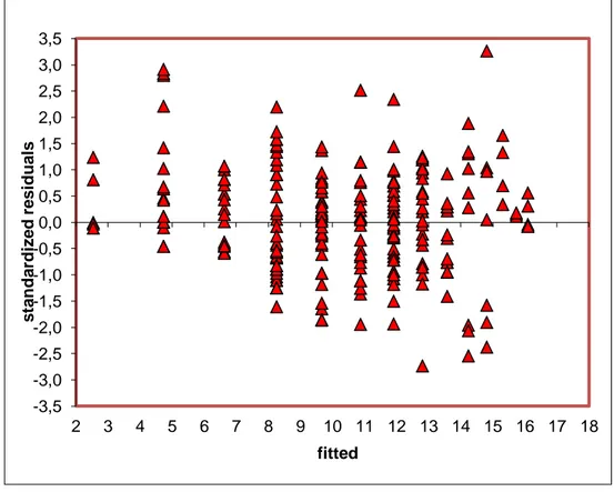
ij we have to consider if the classical assumption are reliable for corals growth.The assumption of zero mean of the error is not called into question as the relationship between the response and the covariate based on the VBGF has a physical meaning and is derived, as already seen, by biochemical considerations. The assumption that the error has common variance σ2 and is identically distributed for all tij
risks to be easily violated for two reasons: the first one is that young corals are less variable than old one as environmental factors have less time to influence them, the second one depends on the way they are measured. The age of solitary corals are determined by counting the growth rings, so in small corals that could be less precise than in adult corals, on the other hand in very old corals, slowing their growth after a certain dimension is very difficult to count ultimate rings because they are very close, sometimes collapsed. The error may be also correlated: the growth in a certain site depends on the yearly fluctuation of environmental parameters, such as temperature, solar radiation and current. So corals closer in age should have had the same fluctuation of environmental parameters.
A more flexible model for the variance of the error can be then build considering the function described in
Errore. L'origine riferimento non è stata trovata. and
Errore. L'origine riferimento non è stata trovata. according to which the error variance matrix becomes
ξ whereξ
' '
' i i R , , , , So that
ξ
ij Ri i, At the inter-site level it is possible to attribute the variations of parameters L∞i and ki among the M sites to
systematic and random sources.
Parameter estimates can be obtained by the method of Least Squares; however minimization of residual sum of squares yields equations nonlinear in the parameters. Since it is not possible to solve nonlinear equations in closed forms, the alternative is to obtain approximate analytic solutions by employing iterative procedures. The main methods being (Draper and Smith 1998): the Taylor Series Method, the Steepest Descend Method and the Levenberg-Marquardt’s Gauss–Newton basedMethod.
It is then possible to see each parameter comprising a fixed effect L∞ and k) due to known site-specific
characteristics and a random effect respectivelyb1i and b2i due to unexplained variation among the sites. The
vector iconsidering both the effect can be then defined
1 2 i i i i i L L b k k b 3.14
Unlike the traditional marine biology approach, the Errore. L'origine riferimento non è stata trovata. approach to parameter estimations has the desirable feature of contemporarily taking into account the site model and the “population” model introducing a hierarchy between them.
Analysis of data of repeated measurement over time is a recurrent challenge to statisticians engaged in biological applications: growth curves are among this kind of data. The inter-individual variability in growth is the result of several internal (genetic) and external (environmental) factors which affect these physiological processes. The choice of applying the growth model to the length-at-collection data rather than
parameters which oversee individual variability in each site of capture. The measures are then repeated in a wide sense. Anyway Pilling et al., (2002) and Schaalje et al., (2001) focused on the statistical nuances of fitting back-calculated lengths at age data in a repeated measures context and obtaining better estimates of individual growth variability than taking repeated measurements on a sample of individuals.
The main strategy followed was to incorporate these features in an inferential setting by building a hierarchical model. Inter-site variation is then considered as consisting of a model for variation in the regression parametersi. Thus variation can be modelled using a distributional assumption for iat various levels of complexity. For instance a possible specification is
A β b
i i i
3.15
where i is assumed to depend linearly on a two-dimensional vector of parameter β and on site-specific information such as temperature and radiation summarized in a design Matrix Ai. as shown further on. Error bi corresponds to the random component of inter-site variation, which is supposed not depending on environmental covariates and is taken to have mean zero and covariance matrix D.
Adding the restriction that the distribution of i belongs to a particular parametric family, the bivariate normal-lognormal distribution is often chosen (Helser and Lai, 2004)
A D i i i i L ( , ) ln k 3.16
So, considering a linear influence of radiation gradient R and temperature gradient Ton L∞ , and exponential
influence of radiation gradient R and temperature gradient Ton k in the parameterization of the VBGF, expression (3.14) is composed by the following elements
0 0 1 0 0 0 0 1 A i i i i i R T R T 3.17 1 2 3 4 ln L a a k a a 3.18 1 2 b i i i b b 3.19
The elements of the bi-dimensional vector-valued function described in
Errore. L'origine riferimento non è stata trovata.are then expressed as
1 1 2 1 2 3 4 2 α β b α β b α i i i i i i i i i i i i i d , , L a R a T b d , , ln( k ) a R a T b R where T 3.203.5.2 The new proposed parameterization
Similarly to the previous chapter the above VBGF Errore. L'origine riferimento non è stata trovata. in accordance with the Errore. L'origine riferimento non è stata trovata. becomes
1 1 1 ci L i ij i t e ij ij i y ( t ) L e j ,..,n i ,.., 3.21
where the error distribution is ij Ri
i,ξ
The i is a bi-dimensional vector , ' i
i L ci
and also in those case it is possible to see each parameter comprising a fixed effect L∞ and cand a random effect b1i and b2i. The vector considering both the effect
can be then defined
1 2 i i i i i L L b c c b 3.22
This new parameterization is designed to be more parsimonious: in fact the two parameters are divided in the one sensitive to environmental and, in general, external, influences that is c and the one derived by genetic and moreover, site not-depending, characteristics, that is L∞.
We consider for the distribution of i the bivariate normal distribution
A β D i i i i L ( , ) c 3.23
Considering a linear influence of radiation (R) and temperature (T) on c which is designed to be the only parameter sensitive to environmental covariates, the parameterization of the VBGF the