Model reduction techniques in flexible multibody dynamics with application to engine cranktrain simulation

(1)

Alma Mater Studiorum – Università di Bologna

DOTTORATO DI RICERCA IN

Meccanica e Scienze Avanzate dell’Ingegneria

Progetto n. 3 - Meccanica Applicata

Ciclo XXV

Settore Concorsuale di afferenza: 09/A2 Settore Scientifico-Disciplinare: ING-IND/13

MODEL REDUCTION TECHNIQUES IN FLEXIBLE

MULTIBODY DYNAMICS WITH APPLICATION

TO ENGINE CRANKTRAIN SIMULATION

Presentata da: Ing. Stefano Ricci

Coordinatore Dottorato: Relatore:

Prof. Vincenzo Parenti Castelli Prof. Alessandro Rivola

(2)

(3)

(4)

(5)

Ringraziamenti

Vorrei innanzitutto ringraziare le persone che hanno contribuito alla realiz-zazione di questa Tesi di Dottorato.

Ringrazio il Prof. Alessandro Rivola, il mio relatore, per avermi dato l’oppor-tunità di lavorare a questo progetto, per la fiducia e per la sua attenta supervisione. Un sentito ringraziamento va al Dott. Marco Troncossi, per la sua disponi-bilità e per il supporto fornito in questi anni. Marco, sarà difficile dimenticare la camminata assurda che abbiamo fatto a Helsinki! Un ringraziamento va anche al Dott. Alberto Martini, con il quale abbiamo condiviso un paio di anni da dottorandi, per i consigli e gli interessanti spunti di discussione.

Un ringraziamento particolare va ai miei colleghi, ed ex-colleghi, della Ducati, in particolare nelle persone di Massimo Rosso, Gabriele Stagni e Michele Mazziotta, per la disponibilità, la simpatia e il supporto nelle fasi iniziali del progetto. Un doveroso grazie anche agli altri miei colleghi per sopportarmi tutti i giorni. . .

Un grazie di cuore a Simone Delvecchio, per l’impagabile amicizia, la sim-patia e la vicinanza nei periodi di difficoltà. Grazie a tutti i miei amici, il cui supporto e la cui stima mi hanno spinto anche quando pensavo di dover desistere.

Un ringraziamento speciale va ai miei genitori e a mio fratello: senza di voi non ce l’avrei mai fatta. Infine a te: grazie per l’amore e l’immenso supporto che mi hai dato in questi anni, e per l’infinita pazienza con la quale mi hai sostenuto in questa esperienza.

Stefano Ricci Bologna, Marzo 2013

(6)

(7)

Abstract

The development of a multibody model of a motorbike engine cranktrain is presented in this work, with an emphasis on flexible component model reduction. A modelling methodology based upon the adoption of non-ideal joints at interface locations, and the inclusion of component flexibility, is developed: both are necessary tasks if one wants to capture dynamic effects which arise in lightweight, high-speed applications.

With regard to the first topic, both a ball bearing model and a journal bearing model are implemented, in order to properly capture the dynamic effects of the main connections in the system: angular contact ball bearings are modelled according to a five-DOF nonlinear scheme in order to grasp the crankshaft main bearings behaviour, while an impedance-based hydrodynamic bearing model is implemented providing an enhanced operation prediction at the conrod big end locations.

Concerning the second matter, flexible models of the crankshaft and the connecting rod are produced. The well-established Craig-Bampton reduction technique is adopted as a general framework to obtain reduced model represen-tations which are suitable for the subsequent multibody analyses. A particular component mode selection procedure is implemented, based on the concept of Effective Interface Mass, allowing an assessment of the accuracy of the reduced models prior to the nonlinear simulation phase. In addition, a procedure to alleviate the effects of modal truncation, based on the Modal Truncation Aug-mentation approach, is developed. In order to assess the performances of the proposed modal reduction schemes, numerical tests are performed onto the crankshaft and the conrod models in both frequency and modal domains.

A multibody model of the cranktrain is eventually assembled and simulated using a commercial software. Numerical results are presented, demonstrating the effectiveness of the implemented flexible model reduction techniques. The advantages over the conventional frequency-based truncation approach are discussed.

(8)

(9)

4.2.1 System description . . . 64 4.2.2 Preliminary simulations . . . 65 4.3 Multibody simulations . . . 67 4.3.1 Model implementation . . . 67 4.3.2 Simulation results . . . 70 4.3.3 Discussion . . . 75 5 Conclusions 79 5.1 Main contributions . . . 79 5.2 Future research . . . 80 Bibliography 83 vi

(11)

(12)

(13)

Chapter 1

Introduction

Modern powertrain design is facing increasingly strict requirements in terms of emissions, fuel consumption, noise and vibration levels. In recent years, this trend is extending towards the motorcycle industry, in which competitive design focused on achieving a high power-to-weight ratio calls for optimized engine components. This in turn requires the adoption of a multidisciplinary approach early in the conception phase, and the use of advanced simulation tools which help the analysts in gaining a deeper insight into the physical phenomena associ-ated with the engine operation.

1.1 Cranktrain dynamics simulation

Concerning structural design aspects, modern analysis techniques involve the adoption of multibody simulation tools, which allow an accurate prediction of loads acting on the system components at operational speed, thus improving the subsequent stress and fatigue life analysis.

Several approaches are described in literature dealing with multibody mod-elling of internal combustion engine powertrains. Some papers deal with the construction of fully coupled cranktrain models through the use of commercial multibody dynamics codes, which provide a general modelling platform for mechanical systems, see e.g. [10, 12, 25, 26, 28, 66, 71, 72, 82, 83]: the system equations of motion are in this case automatically generated by the software kernel, and solved by means of some standard integration scheme. As an alter-native, some studies describe the development of specialized modelling codes, see e.g. [14, 24, 27, 47, 58, 61, 68, 69, 70]: the system equations of motion are retrieved analytically and implemented in specific computational algorithms.

(14)

In this work, the former approach has been followed to investigate the elas-todynamic behaviour of the cranktrain of a Ducati L-twin, four strokes engine, having a displacement of 1.2 litres, capable of delivering 180 horsepower.

In the context of multibody modelling, the definition of a system made up of rigid links connected to each other via kinematic joints typically represents the first step in the process; in fact, commercial multibody software platforms offer both geometry and joint libraries, permitting the analyst to set up a basic dynamic model with little time and effort. Clearly, this modelling approach is affected by some important limitations: first of all, the adoption of rigid bod-ies in combination with kinematic joints prevents some interface loads to be evaluated whenever the mechanism under study exhibits some static indetermi-nacy; furthermore, any dynamic amplification effect, which might significantly affect the actual loads, is evidently lost. These shortcomings can be eliminated by embracing a refined modelling methodology, based upon the introduction of non-ideal joints at interface locations, and the inclusion of component flexibility.

In this study both a ball bearing model and a journal bearing model have been implemented, starting from available literature descriptions, in order to properly capture the dynamic effects of the main connections in the system under study: in fact, the crankshaft is supported by four main journals, three of which equipped with ball bearings, the other one with a bush bearing, while the two connecting rods act on the crankpin through hydrodynamically lubricated journal bearings.

Several ball bearing models are found in literature, mainly referring to dif-ferent approaches: a numerical approach, see e.g. [2, 13, 20, 48, 51], for which the discrete ball-race loads are summed numerically, and an analytical approach, cf. [41, 49], for which the summation of ball-race loads is replaced by an integra-tion. While the former is considered superior in terms of accuracy, the latter is often more accessible for designers who want to include bearing models in their application codes in order to predict bearing performances without having to perform heavy numerical calculations.

The angular contact ball bearing model proposed in [41] is adopted here: the model provides a nonlinear definition of loads and moments acting on the inner ring taking into account five relative race displacements, i.e. three translations and two tilting angles; a full coupling between those is considered.

Concerning journal bearings, their importance in rotating and reciprocating machine applications is proved by the huge number of papers published on this subject. Numerical methods, especially the Finite Element Method (FEM), are widely used to analyse journal bearings including oil feed holes and grooves, and geometry effects like taper and misalignment; such methods, see e.g. [6,

(15)

Cranktrain dynamics simulation ₃

9, 27, 36, 56, 57], are probably the most accurate and versatile, but they tend to be expensive and not always practical. Often, designers use less expensive, approximate analytical methods, cf. [7, 8, 15, 35, 46]; amongst those, the mobility method and its dual counterpart, the impedance method, are the most popular. The impedance description as proposed in [15] for plain, circumferentially-symmetric fluid journal bearings is taken here as reference. Such a model pro-vides a dynamic nonlinear definition of the bearing reaction force as a function of the journal motion, being particularly suited for transient simulation work. The adopted formulation is a combination of the two asymptotic short bearing and long bearing solutions [65], and performs well for general finite-length bear-ings at both large and small eccentricity ratios; furthermore, since the pressure distributions are not calculated, the method permits very efficient computation.

Specific computational routines have been produced concerning both bear-ing types, and embedded into the adopted multibody solver.

As mentioned, another key aspect in obtaining realistic results from multi-body dynamic simulations is the inclusion of component flexibility: this is a necessary task if one wants to capture dynamic effects which arise in lightweight, high-speed applications.

Different techniques exist to incorporate body flexibility in multibody mod-els [75, 80]; among those, the Floating Frame of Reference formulation is certainly the most widely used, and is currently implemented in several commercial multi-body dynamics software packages. The assumption here is that the deformation of the generic flexible body keeps small with respect to a body local reference frame, which in turn undergoes large, nonlinear motion relative to an inertial global reference frame; such hypothesis of linear body flexibility allows linear model reduction techniques to be exploited to reduce the number of coordinates required to describe the component deformation, thus reducing the needed computational effort.

In particular, Component Mode Synthesis (CMS) techniques can be em-ployed to describe body deformation as a linear combination of a number of mode shapes: this task is accomplished by means of some coordinate trans-formation, from physical to modal domain, which can include different kind of modes [16, 17], i.e. eigenmodes, constraint modes, attachment modes, etc. With this respect, several schemes were proposed by a number of authors in the past, see e.g. [18, 42, 45, 50, 62, 73, 74]; due to a simple, straightforward for-mulation of the reduction process, combined with good overall performance, the Craig-Bampton (CB) approach [18] has gained increasing popularity among the structural dynamics community, and is nowadays the most widely used reduction method for flexible multibody dynamics applications.

(16)

Such method has been employed here as a general framework to obtain reduced model representations for both the crankshaft and the connecting rods involved in the cranktrain under study.

1.2 Focus of the thesis

Model reduction through CMS implies that the full set of physical coordinates is reduced to a smaller set of generalized coordinates, giving rise to a modal selection problem. Clearly, the two most important aspects of such a problem are model order and model accuracy: an optimal reduction would result in the minimal set of component modes which ensures acceptable accuracy in the simulation results. Despite modal selection being an important concern in CMS techniques, and CB in particular, not many papers exist on the subject, and the standard practice consists in using some frequency-based criterion to select mode shapes to retain in the reduced representation of a component.

In the present work, a different approach is proposed: the mode selection procedure is carried out in accordance with a modal ordering scheme based upon Effective Interface Mass (EIM), which determines the contribution of each mode shape to the dynamic loads at the interface, providing a rigorous measure of modal dynamic importance. The EIM approach was introduced in the mid-nineties [54, 55], with main focus on dynamic substructuring and control-structure interaction applications; an extension towards multibody dynamics is presented here.

The dual aspect of modal selection is modal truncation: modes which are not retained in the reduced representation of a component are simply discarded. This might lead to inaccurate representation of the applied loading, both concerning its time dependency and its spatial dependency [21]: while the first concern is usually addressed by including in the reduced representation a number of modes spanning a multiple of the frequency range of interest, the latter is often ignored. Some techniques were proposed in the past to tackle this problem, being the Mode Acceleration method [19] the most popular one: such method, however, acts only at the physical response recovery stage, and does not provide any enhancement to the modal representation of the component.

In the present study, the Modal Truncation Augmentation (MTA) tech-nique [21, 23, 31] is adopted to augment the CB reduction transformation matrix with a set of pseudo-eigenvectors, which provide a quasi-static correction for low-frequency excitation, as well as a dynamic correction for high-frequency excitation. Unlike Mode Acceleration, the enhancement impacts the dynamic characteristics of the reduced flexible component, thus resulting attractive for

(17)

Outline of the dissertation ₅

multibody dynamics applications.

Both the EIM and the MTA techniques have been implemented as specific routines within the adopted FE commercial code, and used to obtain reduced models of both the crankshaft and the connecting rod employed for the subse-quent multibody dynamic simulations.

1.3 Outline of the dissertation

This thesis is organized as follows.

Chapter 1 introduces the thesis by presenting the subject, highlighting the main focus and clarifying the organization of the text.

Chapter 2 presents the ball bearing and journal bearing models employed for simulation purposes, describing the theoretical developments of the models and providing some details about their specific implementation in the multibody dynamics software.

Chapter 3 discusses the component model reduction techniques which are used to obtain reduced flexible component models of the crankshaft and the connecting rod. The theoretical developments of the CB, EIM and MTA methods are provided, along with the details about their practical implementation in the FE code. The assessment of the reduced models through numerical tests performed onto the single components is eventually described.

Chapter 4 presents the development of the multibody model of the engine cranktrain. A brief theoretical overview about the Floating Frame of Reference formulation in flexible multibody dynamics is provided first. The multibody model assembly is then described, and the specific simulation results are dis-cussed demonstrating the benefits of the adopted model reduction techniques.

Chapter 5 provides some concluding remarks and suggestions for future research.

(18)

(19)

Chapter 2

Bearing modelling

The use of ideal joints, i.e. kinematic constraints, is a standard practice in multi-body dynamics simulation, especially when commercial software platforms are employed for the purpose: these usually provide ready-to-use joint libraries from which the user selects the most suitable ones for his specific application, allowing for an express model deployment. Whenever accuracy is a major con-cern, however, this modelling approach is somewhat restrictive, and the use of non-ideal joints, i.e. force constraints, should be taken into consideration for the main connections in the system. Clearly this requires the additional effort of implementing joint models, which can be an expensive activity depending on the complexity of the involved theoretical background; furthermore, dynamic simulations including such kind of models can be costly, thus a cost-benefit analysis should always be made to choose adequate modelling strategies.

In this study both a ball bearing model and a journal bearing model have been implemented, starting from available literature descriptions, in order to properly capture the dynamic effects of the main connections in the cranktrain under study, cf. Chapter 4: in fact, the crankshaft is supported by four main journals, three of which equipped with ball bearings, the other one with a bush bearing, while the two connecting rods act on the crankpin through hydrodynamically lubricated journal bearings.

2.1 Ball bearing modelling

Several ball bearing models are found in literature, mainly referring to different approaches: a numerical approach, see e.g. [2, 13, 20, 48, 51], for which the discrete ball-race loads are summed numerically, and an analytical approach, cf. [41, 49], for which the summation of ball-race loads is replaced by an integration.

(20)

While the former is considered superior in terms of accuracy, the latter is often more accessible for designers who want to include bearing models in their application codes in order to predict bearing performances without having to perform heavy numerical calculations. The method proposed by Hernot et al. [41] is adopted here, this consisting actually in a matrix formulation of Houpert’s uniform analytical approach [49], based on a first-order development of the ball-race Hertzian deformation.

Hertzian theory refers to the localized stresses that develop as the generic bearing ball comes in contact with the inner and outer raceways, slightly de-forming under the imposed loads. Such deformations, assumed as elastic, are small compared to the dimensions of the contact area, which, in turn, is consid-ered to be small with respect to the radii of curvature of the contacting bodies. No deformation of the inner and outer rings occur, except at the balls contact area: the stiffness of the whole bearing can be seen as a result of the stiffnesses associated to each ball-raceway contact. The load on each rolling element is assumed to be normal to the contacting surfaces, and the effects of surface shear stresses are neglected: the direction of such load identifies the contact angle, that defines the ability of angular contact bearings to support thrust loads and that does not usually exceed 40 degrees. Such angle is assumed as a constant throughout the mentioned references [41, 49]: any variation caused by imposed loads or centrifugal effects is ignored. In very high speed applications, though, such hypothesis becomes too strict, and models taking into account a contact angle variation must be employed [3, 59, 60].

The model presented here provides a nonlinear definition of loads and mo-ments acting on the inner ring taking into account five relative race displace-ments, i.e. three translations and two tilting angles; a full coupling between those is considered. No radial clearances within the bearing, nor thermal effects are included; furthermore, the influence of the lubrication film is ignored.

2.1.1 Theoretical background

In order to clarify how the matrix formulation has been obtained in [41], the 2-degrees-of-freedom (2-DOF) ball bearing model is reviewed first. This model neglects any misalignment between inner and outer ring axes, which are thus considered to remain parallel under load. Such load, which can be expressed as a superposition of a thrust load Fa_{and a radial load F}r_{, determines a displacement}

of the inner ring with respect to the outer ring, which will be considered as fixed hereinafter. The variation of the distance between inner and outer ring can be approximated as a combination of an axial displacement, δa, and a displacement

(21)

Ball bearing modelling ₉

Figure 2.1 Angular contact ball bearing parameters, adapted from [41]

along the radial load direction, δr, as:

d

ψ ≈ δa_{sin α + δ}r_{cos α cos ψ} _(2.1)

where α is the bearing contact angle, see Figure 2.1, while ψ defines the generic rolling element angular position with respect to the radial load direction. This ap-proximation ignores any contact angle variation, which is commonly acceptable for bearing analysis provided that both δaand δrare very small when compared

to the overall bearing dimensions. The ball-race deflection is given by:

δψ = max (0, dψ) (2.2)

since compression only occurs for positive values of dψ.

The ball-raceway contact load Q is estimated using the traditional Hertzian load-deflection relationship:

Q = kδn (2.3)

where k is a factor depending on the contact geometry and the material elastic constants. The exponent n only depends upon the contact geometry: for ball bearings, where point contact can be assumed, n = 3⁄2 . The contact load at any angular position is then given by:

Qψ = k [max (0, dψ)] n

(22)

which can be rearranged as:

Qψ = kdψ[max (0, dψ)] n−1

(2.5)

This simple step is crucial towards the definition of a matrix formulation of the problem.

For static equilibrium to exist, the summation of rolling element forces in each direction must equal the applied load in that direction:

Fa= 2π ∑ ψ=0 Qψsin α (2.6a) Fr = 2π ∑ ψ=0 Qψcos ψ cos α (2.6b)

If equation (2.5) is used instead of (2.4), then the previous can be rearranged in matrix format as:

{Fa Fr} = [K 11 K12 K12 K22 ] {δa δr} (2.7) with: K11= 2π ∑ ψ=0 k[max (0, d ψ)] n−1 sin2α (2.8a) K12= 2π ∑ ψ=0 k[max (0, d ψ)] n−1

cos ψ sin α cos α (2.8b)

K22= 2π ∑ ψ=0 k[max (0, d ψ)] n−1 cos2ψ cos2α (2.8c)

Since the angular position of the balls changes during normal operation, the stiffness of the bearing also changes continuously in real-life applications. In order to avoid taking into account the angular position of each ball, which would result in an increased model complexity, it is possible to use the integral form of Sjoväll [39, 77]: this prevents summing the discrete rolling element loads, by making the assumption that the angular position of the rolling elements with respect to each other is always maintained due to a rigid, ideal cage. The expressions of the bearing stiffness matrix elements in (2.8) may then be rewritten as:

(23)

Ball bearing modelling ₁₁

K12= Kεsin α cos α Jra(ε) (2.9b)

K22= Kεcos2α Jrr(ε) (2.9c)

being Kεa stiffness dimensional factor:

Kε= Zk (δasin α + δrcos α) n−1

(2.10)

Here, Z is the number of rolling elements. The integrals in (2.9) can be expressed as: Jaa(ε) = 1 2π∫ 2π 0 H (ε) dψ (2.11a) Jra(ε) = 1 2π∫ 2π 0 H (ε) cos ψdψ (2.11b) Jrr(ε) = 1 2π∫ 2π 0 H (ε) cos 2 ψdψ (2.11c) where: H (ε) = [max (0, 1 −1 − cos ψ 2ε )] n−1 (2.12)

The load distribution factor ε is defined as:

ε = 1 2(1 +

δa_{tan α}

δr ) (2.13)

The integrals in (2.11) may be evaluated numerically for any value of ε; Hernot proposed approximate equations which precisely fit these numerical results [41], and which allow an easier implementation.

Let’s now extend the explained concepts to the 5-DOF model. In this case the distance variation between inner and outer race has been calculated by Houpert [49] by taking into account five relative displacements, i.e. three translations and two tilting angles. The exact relationship is rather cumbersome, but Houpert used a first-order development to obtain a simplified relationship:

d

φ≈ δxsin α + ∆ycos α cos φ + ∆zcos α sin φ (2.14)

where ∆y_{, ∆}z_{are the equivalent radial displacement components along the global}

y and z axes:

∆y = δy− δ_θz_Ri_{tan α} _(2.15a)

(24)

Figure 2.2 Coordinate system used for the 5-DOF model, adapted from [41]

Here, Riis the mean inner race radius1, while φ is the generic rolling element

angular position with respect to the y axis, see Figure 2.2. The equivalent radial displacement can be expressed as:

∆r=

√

∆2y+ ∆2z (2.16)

so that (2.14) can be rewritten:

d

φ≈ δxsin α + ∆rcos α cos (φ − φr) (2.17)

In the previous, φrrepresents the direction of the maximum radial displacement

and is defined as:

φr=⎧⎪⎪⎨⎪⎪

⎩

arctan (∆z/∆y) , ∆y≥ 0

arctan (∆z/∆y) + π, ∆y< 0

(2.18)

Note that there is a complete analogy between (2.17) and (2.1).

The static equilibrium between rolling element forces and applied loads now holds: Fx= 2π ∑ φ=0 Qφsin α (2.19a) Fy= 2π ∑ φ=0 Qφcos φ cos α (2.19b) 1

Houpert derived expression (2.14) by using the mean inner race radius Ri_{, see Figure 2.1,}

while Hernot uses the radius of the intersection between the contact cone and the inner raceway median plane, RI, throughout [41]. The former has been taken here as reference, but it seems

(25)

Ball bearing modelling ₁₃ Fz= 2π ∑ φ=0 Qφsin φ cos α (2.19c) My = Fz_Ri_{tan α} _(2.19d) Mz= −FyRitan α (2.19e)

where the ball-raceway contact load distribution Qφhas been introduced. By

expressing it in a similar fashion to that in (2.5) allows to rearrange (2.19) in matrix format, in complete analogy with the described two-DOF bearing model. The load-displacement relationship becomes:

⎧⎪⎪⎪ ⎪⎪⎪⎪⎪ ⎨⎪⎪ ⎪⎪⎪⎪⎪ ⎪⎩ Fx Fy Fz My Mz ⎫⎪⎪⎪ ⎪⎪⎪⎪⎪ ⎬⎪⎪ ⎪⎪⎪⎪⎪ ⎪⎭ = ⎡⎢ ⎢⎢ ⎢⎢ ⎢⎢ ⎢⎢ ⎣ K11 K12 K13 K14 K15 K22 K23 K24 K25 K33 K34 K35 Sym K44 K45 K55 ⎤⎥ ⎥⎥ ⎥⎥ ⎥⎥ ⎥⎥ ⎦ ⎧⎪⎪⎪ ⎪⎪⎪⎪⎪ ⎨⎪⎪ ⎪⎪⎪⎪⎪ ⎪⎩ δx δy δz δθ y δθz ⎫⎪⎪⎪ ⎪⎪⎪⎪⎪ ⎬⎪⎪ ⎪⎪⎪⎪⎪ ⎪⎭ (2.20) with: K11= Kεsin2α Jaa(ε) (2.21a)

K12= Kεsin α cos α cos φr Jra(ε) (2.21b)

K13= Kεsin α cos α sin φr Jra(ε) (2.21c)

K14= K13Ri_{tan α} _(2.21d)

K15= −K12Ritan α (2.21e)

K22= Kεcos2α [sin2φr Jaa(ε) + cos 2φr Jrr(ε)] (2.21f )

K23= Kεcos2α sin 2φr[Jrr(ε) − 1

2J

aa(ε)] (2.21g)

K24= K23Ritan α (2.21h)

K25= −K22Ritan α (2.21i)

K33= Kεcos2α [cos2φr _Jaa(ε) − cos 2φr _Jrr(ε)] _(2.21j)

K34= K33Ritan α (2.21k)

K35= −K23Ritan α (2.21l)

K44= K33R2itan2α (2.21m)

K45= −K23R2itan2α (2.21n)

K55= K22R2i tan2α (2.21o)

The integral function expressions in (2.11) are still valid, as well as the stiffness dimensional factor in (2.10) and the load distribution factor in (2.13), provided

(26)

that the axial and radial displacements δaand δrare now replaced by the

corre-sponding variables δxand ∆r.

2.1.2 Model implementation

The described 5-DOF bearing model has been implemented in ADAMS by using the field element, which computes forces and moments acting between any two markers, i.e. reference frames, based upon their relative displacements and velocities. Full 6-by-6 stiffness and damping matrices can be defined for the purpose; preloads are allowed, as well.

In the present case, dealing with a nonlinear model, the mentioned matrices need to be computed by means of a fiesub user-written subroutine; this has been coded in Fortran, and its basic functioning is briefly depicted in the following. Model parameters are the angular bearing contact angle α, the mean inner race radius Ri_{, obtained from pure geometrical considerations, the number of}

rolling elements Z, as from the bearing specifications, and the load-deflection factor k, which can be approximated as2:

k≈ 105

D1/2 (2.22)

being D the rated ball diameter. The presented formulation has been enriched by adding damping, so that (2.20) becomes, using compact notation:

F = K (δ + c ˙δ) (2.23)

resulting in a proportional damping formulation; the damping constant c is a user-defined parameter.

Model inputs are the relative displacements and velocities of the markers attached to the inner and outer rings3, δ and ˙δ, evaluated at each simulation timestep, from which the equivalent radial displacement ∆rand its direction

φrare readily computed, along with the load distribution factor ε. The stiffness

dimensional factor and the load distribution integrals are then computed accord-ing to (2.10) and (2.11), respectively; attention has been paid to the definition of

2

Such approximation holds true, according to [41], for 7200 and 7300 angular contact ball bearing series; for other bearing types information should be gathered from available literature, or directly from the manufacturer.

3

The field element only allows the angle about the z axis to become arbitrarily large during a simulation, the others having to remain smaller than 10 degrees: to keep the original formulation as in [41], an input and output “switch” has been implemented, mapping the ADAMS model coordinates to the reference frame used in the bearing model definition, cf. Figure 2.2. Obviously, the markers in the model have to be oriented accordingly, i.e. z along the axial direction and x, y in the radial ones.

(27)

Journal bearing modelling ₁₅

those cases which might give rise to numerical issues, e.g. ∆r = 0 or ε ≤ 0, for

which the proper values are simply assigned to the aforementioned variables. The stiffness matrix elements are eventually computed according to (2.21), and use to calculate the force vector F. In addition to the force vector components, the fiesub element requires as output arguments the derivatives of those with respect to both the displacement variables in δ and the velocity variables in

˙

δ; these partial derivatives have been evaluated analytically with the aid of a symbolic math manipulation software, and included in the Fortran code.

2.2 Journal bearing modelling

Concerning journal bearings, their importance in rotating and reciprocating machine applications is proved by the huge number of papers published on this subject. Numerical methods, especially the Finite Element Method, are widely used to analyse journal bearings including oil feed holes and grooves, and geometry effects like taper and misalignment; such methods, see e.g. [6, 9, 27, 36, 56, 57], are probably the most accurate and versatile, but they tend to be expensive and not always practical. Often, designers use less expensive, approximate analytical methods, cf. [7, 8, 15, 35, 46]; amongst those, the mobility method and its dual counterpart, the impedance method, are the most popular.

The concept of mobility was introduced by Booker [7] to address the problem of determining the motion of the bearing journal given the applied force: such approach is applicable for bearings for which the external load is known and dominant with respect to the inertia effects of the rotor, and found its preferred field of application in the analysis of journal bearings employed in reciprocating machines, such as internal combustion engines. The dual concept of impedance was later introduced by Childs et al. [15] to solve the problem of determining the bearing reaction force given the position and velocity of the journal: this approach is more suited to those problems where the stiffness and inertia prop-erties of the rotor must be accounted for, resulting preferred in rotordynamic analysis.

The impedance description as proposed in [15] for plain, circumferentially-symmetric fluid journal bearings is taken here as reference. Such a model pro-vides a dynamic nonlinear definition of the bearing reaction force as a function of the journal motion, being particularly suited for transient simulation work. The adopted formulation is a combination of the two asymptotic short and long solutions [65], and performs well for general finite-length bearings at both large and small eccentricity ratios; furthermore, since the pressure distributions are not calculated, the method permits very efficient computation.

(28)

2.2.1 Theoretical background

This section briefly presents the theoretical development of the impedance method [15].

The hydrodynamic lubrication theory is based on the well-known Reynolds equation. If variations of viscosity are ignored, and if the lubricant is assumed as incompressible, such equation simplifies to:

∂ ∂θ(h 3∂ p ∂θ) + R 2 ∂ ∂z(h 3∂ p ∂z) = 12µR2 C2 [˙ε cos θ + ε (˙β − ω) sin θ] (2.24)

where θ and z are the angular and the axial cylindrical coordinates, respectively. R and C are the rated bearing radius and radial clearance, respectively, ε is the eccentricity ratio, i.e. the journal center eccentricity e normalized to the radial clearance, while h is the normalized film thickness defined as:

h= 1 + ε cos θ _(2.25)

The angle β defines the direction of eccentricity, see Figure 2.3, while ω is the aver-age angular velocity of journal and sleeve with respect to a grounded, stationary frame:

ω = 1 2(ω

j+ ωs) (2.26)

Figure 2.3 Kinematic variables for impedance and mobility definitions, adapted

(29)

Journal bearing modelling ₁₇

Finally, µ and p are the fluid viscosity and film pressure, respectively.

Considering now an observer pinned to the sleeve center and rotating at the angular velocity ω, the actual journal center velocity ˙e and the velocity Vs

apparent to the observer are related by the simple kinematic expression:

Vs= ˙e − ω × e (2.27)

where the vector notation has been introduced; the symbol × indicates cross product. Since the average angular velocity of journal and sleeve apparent to the observer would vanish identically, the generation of pressure would seem to be related solely to the apparent velocity Vs_{in exactly the same way as for}

a non-rotating journal: such velocity Vs is henceforth called effective squeeze

velocity, and the corresponding pressure equals the pressure generated by the combined effect of the actual squeeze velocity ˙e and the wedge effect due to the rotation of journal and sleeve, cf. Figure 2.4.

The Reynolds equation (2.24) might be rewritten in terms of the effective squeeze velocity as:

∂ ∂θ(h 3∂ p ∂θ) + R 2 ∂ ∂z(h 3∂ p ∂z) = 12µVsR2 C3 cos (α + θ) (2.28)

where α represents the attitude angle of the eccentricity vector with respect to the effective squeeze velocity vector, see Figure 2.3. An analytical solution of (2.28) for arbitrary geometry cylindrical bearings is not feasible. Most frequently, numerical methods are employed to solve such equation and to obtain the perfor-mance characteristics of bearing configurations of particular interest. However, approximate analytical solutions can be obtained by a direct integration of (2.28) under different assumptions.

(30)

The Ocvirk solution is obtained by ignoring the pressure variations in the circumferential direction, and solving for p(θ, z) with the axial boundary con-dition of zero relative pressure at both bearing ends. Integrating axially yields the following average axial film pressure:

p(θ) = −µVsL

2

h3_C3 cos (α + θ) (2.29)

being L the bearing axial length. The pressure is seen to be positive between the angles:

θ1=

π

2− α (2.30a)

θ2= θ1+ π (2.30b)

The assumption is made that the pressure gradient along θ is negligible with respect to that along z, which is equivalent to consider the bearing as infinitely short: the model is also referred to as short bearing solution, and is generally applicable for narrow bearings characterized by slenderness ratios, i.e. length-to-diameter, up to 0.5.

The Sommerfeld solution is obtained by neglecting the pressure variations in the axial direction, and solving for p (θ) with the boundary condition of 2π-periodicity with respect to θ and the requirement that the positive pressure sector extends over π radians, providing:

p(θ) = −6µVsR

2

h2_C3 (cos α cos θ − b sin α sin θ) (2 + ε cos θ) (2.31)

where

b= 2

2 + ε2 (2.32)

The positive pressure sector lies between the angles defined by:

tan θ1=

1

b tan α (2.33a)

θ2= θ1+ π (2.33b)

The assumption here is that the fluid pressure is constant along z and that leakage at bearing ends is negligible, which is equivalent to consider the bearing as infinitely long: the model is also referred to as long bearing solution, and applies for slenderness ratios greater than 2. An extension is provided by the Warner-Sommerfeld model, which is obtained by multiplying the Warner-Sommerfeld pressure

(31)

Journal bearing modelling ₁₉

distribution by an end-leakage function varying only in the axial direction: the effects of both circumferential and axial pressure variations are considered, generally leading to more satisfactory results.

These asymptotic solutions have demonstrated a restricted range of appli-cation. For short bearings the Ocvirk solution has proven to be accurate in defining the direction of the bearing reaction, but predicts an erroneously large magnitude especially at large eccentricity ratios. The Sommerfeld model, as well as the Warner-Sommerfeld one, provides an improved definition of the bearing reaction magnitude for long bearings and high eccentricity ratios, but leads to inaccurate definition of its direction. The fact that their ranges of application do not coincide, allows the two models to be combined in such a way to obtain approximate solutions valid for general finite-length bearings at both small and large eccentricity ratios.

The forces acting on the journal can now be derived by integrating the ob-tained pressure distribution, e.g. (2.29, 2.31). This integration can be performed over the entire angular domain, leading to a complete film condition (Sommer-feld, or full, or 2π boundary condition) which justifies the presence of negative pressures within the fluid film, or only over the positive portion of the pressure distribution, leading to a ruptured film condition (Gümbel, or half, or π boundary condition) that prevents the development of negative pressures, see Figure 2.5: while the former neglects any phase effects, the latter provides an approximate model for cavitation and tends to be more generally applicable, leading to more realistic predictions. Actually, the π boundary condition is not correct as it vio-lates the continuity of the flow across the cavitation boundary; other boundary condition sets which remove this inconsistency exist, see [79], but they tend to be much more sophisticated and cumbersome to implement in practice.

Integration of the pressure distribution yields the components of the force F acting from the fluid film on the journal. The impedance method permits

(32)

to avoid such integration to compute the reaction force, removing the need of calculating the actual pressure distribution. The dimensionless impedance vector is defined by:

W = (C/R)3 2µL

F_L

Vs (2.34)

where the vector FL is the force applied from the journal to the fluid film, as

opposed to the mentioned bearing reaction force, F = −FL. For the sake of

completeness, let’s recall the mobility definition, as well:

M = 2µL

(C/R)3

Vs

FL

(2.35)

From the previous, impedance and mobility appear as the dimensionless counter-parts of force and effective squeeze velocity, respectively; clearly, their magnitudes are reciprocal.

Several analytic mobility and impedance definitions were derived in the past, either analytically or by fitting numerical results, relating to either short, long or finite-length bearings under complete or ruptured fluid film conditions. By using these definitions, it is a simple matter to compute the journal velocity starting from the knowledge of applied force and eccentricity (mobility approach), or the bearing reaction force starting from journal position and velocity (impedance approach). Transformation from a mobility definition to an impedance definition can be carried out by the following relationships:

tan α = −Mβ(ε, γ) Mε(ε, γ) (2.36) tan γ = −Wβ(ε, α) Wε(ε, α) (2.37)

together with the reciprocity relation between mobility and impedance magni-tudes. The angle γ defines the orientation of the eccentricity with respect to the impedance vector, see Figure 2.3.

In the present work, a π finite-lenght impedance description has been used [15], which is based on a mobility definition obtained as a weighted sum of the Ocvirk and Sommerfeld solutions, and which provides good approximation for all eccentricities and L/D ratios. The amplitude of the impedance vector is expressed as:

W = [0.15 (E2+ G2)1/2(1 − ε cos γ)3/2]

−1

(33)

Journal bearing modelling ₂₁ where: E = 1 + 2.12Q (2.39a) G =3ε sin γ (1 + 3.6Q) 4 (1 − ε cos γ) (2.39b) Q = 1 − ε cos γ (L/D)2 (2.39c)

The angle γ can be obtained from the approximate solution:

γ ≈⎛ ⎝1 − ε cos α √ 1 − η2 ⎞ ⎠(arctan A + arcsin η − π η 2 ∣η∣) − arcsin η + α (2.40) being: η = ε sin α (2.41a) A =4 (1 + 2.12B) √ 1 − η2 3η (1 + 3.6B) (2.41b) B = 1 − ε 2 (L/D)2 (2.41c)

Further details can be found in reference [15].

2.2.2 Model implementation

The described bearing model has been implemented in ADAMS by using the gforce element, which allows defining functions that represent the three trans-lational and three rotational vector components of a generalized force vector acting between any two defined markers. Since, in the present case, the force ex-pressions require a quite cumbersome definition, their computation is performed through a gfosub user-written subroutine; this has been coded in Fortran, and its basic functioning is briefly depicted in the following.

Model parameters are the bearing axial length L, the bearing diameter D and the radial clearance C, along with the dynamic viscosity of the lubricant µ evaluated at operating temperature (the algorithm neglects any thermal effects).

Inputs of the model are the displacements and velocities of the journal relative to the sleeve, evaluated at each integration step, as well as the angular velocities of both journal and sleeve, expressed with respect to a grounded, stationary reference marker.

The eccentricity vector in both magnitude ε and direction β is computed first, along with the average angular velocity ω. The effective squeeze velocity vector

(34)

is then computed according to (2.27), from which magnitude Vsand direction ζ

are readily available. The angle defining the eccentricity vector with respect to the effective squeeze velocity vector can thus be evaluated according to Figure 2.3 as:

α = β − ζ (2.42)

The angle γ defining the orientation of the eccentricity vector with respect to the impedance vector is now computed according to (2.40, 2.41), so that the impedance vector magnitude can now be derived as in (2.38, 2.39). The direction of the impedance vector with respect to the pure-squeeze-velocity vector is defined by the angle:

ψ = α − γ (2.43)

Now that the impedance vector is known in both magnitude and direction, the force on the journal can be computed according to (2.34).

It is worth mentioning that the described model cannot handle impacts between the journal and the bearing surface: if that circumstance occurs during the simulation run, the process is stopped and a warning message is issued. Such limitation could be overcome by implementing some dry contact model, along with a proper transition mechanism between that and the adopted hydrodynamic force model, see e.g. [29, 30].

(35)

Chapter 3

Component model reduction

In multibody systems, the inclusion of component flexibility is a necessary task if one wants to capture dynamic effects which arise in high-speed applications. According to the widespread floating frame of reference approach [76], the mo-tion of each flexible body is subdivided into a reference momo-tion, which can be described according to rigid multibody formalism, and a deformation. The Finite Element Method (FEM) is commonly used to describe such deformation; since small displacements and rotations are assumed to occur about the floating frame, linear methods borrowed from structural dynamics can be exploited, such as Component Mode Synthesis (CMS) techniques, in order to reduce the number of coordinates required to describe the component deformation. This task is accomplished by means of some coordinate transformation, from physical to modal domain, which involves the definition of proper component mode shapes; the reduction basis can include any sort of modes [16, 17], i.e. eigenmodes, con-straint modes, attachment modes, etc., which were combined in several ways by a number of authors in the past [18, 42, 45, 50, 62, 73, 74]. Due to a simple, straightforward formulation of the reduction process, combined with good over-all performance, the Craig-Bampton (CB) approach [18] has been widely used in structural dynamics, and is largely the most popular CMS method amongst the multibody dynamics community. This method is available in most commercial FE codes, and is generally considered as a standard for inclusion of component flexibility into multibody simulation work. Therefore, it has been employed as a general framework for component model reduction in the present study.

Until some kind of loading is applied, either transient or frequency response, it is very difficult to predict which modes will play a dominant role in the response of the structure. Model reduction, however, implies that the full set of physical coordinates is reduced to a smaller set of generalized coordinates, giving rise

(36)

to a modal selection problem. Clearly, the two most important aspects of such a problem are model order and model accuracy: an optimal reduction would result in the minimal set of component modes which ensures acceptable accuracy in the simulation results. Despite modal selection being an important concern in CMS techniques, and CB in particular, not many papers exist on the subject. Spanos et al. [78] developed a two-stage mode selection procedure derived from balanced realization theory [67]: the CB representation of the component is generated first, then brought to diagonal form and eventually further reduced via balancing; this is performed by using Gregory’s [37] modal ranking criterion derived for lightly damped structures with well separated modal frequencies. In the present work, a selection procedure carried out in accordance with a modal ordering scheme based on Effective Interface Mass (EIM) is adopted. The EIM approach was introduced by Kammer et al. [54] in the mid-nineties, with main focus on dynamic substructuring and control-structure interaction applications; an extension towards multibody dynamics is proposed here.

The dual aspect of modal selection is modal truncation: component modes which are not retained in the reduced representation are simply discarded. This might lead to inaccurate representation of the applied loading, both concerning its time dependency and its spatial dependency [21]: while the first concern is usually addressed by including in the reduced representation a number of modes spanning a multiple of the frequency range of interest, the latter is often ignored. Some techniques were proposed in the past to tackle this problem, being the Mode Acceleration (MA) method [19] the most popular one: such method, however, acts only at the physical response recovery stage, and does not provide any enhancement to the modal representation of the component. In the present study, the Modal Truncation Augmentation (MTA) technique [21, 23, 31] is adopted to augment the CB reduction transformation matrix with a set of pseudo-eigenvectors, which provide a quasi-static correction for low-frequency excitation, as well as a dynamic correction for high-frequency excitation. Un-like MA, the enhancement impacts the dynamic characteristics of the reduced component, thus resulting attractive for multibody dynamics applications.

3.1 Theoretical background

3.1.1 The Craig-Bampton approach

This section briefly presents the theoretical development of the Craig-Bampton (CB) reduction method [18].

(37)

Theoretical background ₂₅

The equilibrium equation for the free-free, undamped structure holds:

M ¨u + K u = f (3.1)

where M and K are the FE mass and stiffness matrices, respectively, and f is the external force vector. The physical degrees of freedom (DOFs) are partitioned into two complementary sets, the interface DOFs (subscript a, “active”) and the interior DOFs (subscript o, “omitted"):

[Maa Mao Moa Moo] { ¨ ua ¨ uo} + [ Kaa Kao Koa Koo] { ua uo} = { fa 0 } (3.2)

Here, it has been assumed that external loads, i.e. external forces/torques, are applied only at the interface DOFs; clearly this requires a proper a-set definition. The following coordinate transformation is then introduced:

{ua uo} = [ I 0 ψoa ϕoq ] {ua q } (3.3)

in which ψoais a matrix of shapes obtained considering the lower partition of

the static portion of (3.2) and solving for the o-set displacements:

uo= − K−1ooKoaua= ψ_oaua (3.4)

while ϕoqis a matrix of shape vectors satisfying the o-set eigenproblem:

Kooϕ_oq= Mooϕ_oqΩ (3.5)

For the sake of compactness, we are now dropping the subscripts defining the dimensions of the matrices ψoaand ϕoq, which will be simply identified by ψ

and ϕ, respectively, in the following.

The first Nacolumns of the transformation matrix in (3.3) represent the static

deformation shapes of the component when subjected to unit displacements at each of the a-set DOFs, the other being restrained; these are termed constraint modes in literature, and constitute the basis for the Guyan static condensation technique [38]. The last Nocolumns are fixed-interface normal modes, i.e.

eigen-vectors, representing the dynamics of the substructure interior relative to the interface; the corresponding eigenvalues, i.e. the squared eigenfrequencies, are collected in the diagonal matrix Ω. As one might notice, the generalized coordi-nate vector comprises both physical displacements, ua_{, and modal displacements,}

q; the fact that interface DOFs are retained in the reduced representation greatly facilitates component coupling, this being probably a major reason for the success of the CB method.

(38)

Introducing the transformation (3.3) into (3.2), and pre-multiplying by the transpose of the transformation matrix, the CB substructure representation is obtained: [Ms − PT − P I ] {¨ ua ¨ q } + [ Ks 0 0 Ω] { ua q } = { fa 0 } (3.6)

where the fixed-interface modes have been normalized with respect to the o-set mass matrix. The following positions hold:

Ms= Maa+ Maoψ + ψTMoa+ ψTMooψ (3.7a)

Ks= Kaa+ Kaoψ _(3.7b)

P = − ϕT_(M

ooψ + Moa) (3.7c)

being Ms_{and K}s_{the statically reduced mass and stiffness matrices, respectively;}

the matrix P is a modal participation factor matrix, containing the multiplication factors for the acceleration inputs at the interface DOFs governing the response of the fixed interface modal coordinates, cf. (3.8).

Most often, the dynamic behaviour of the FE component in a certain fre-quency range of interest can be captured using a much smaller number of gener-alized coordinates compared with the original number of physical coordinates: there lies model reduction. The selection of modes to include in the CB trans-formation matrix (3.3) plays a central role in the application of the method. The definition of the constraint modes directly comes from the coordinate parti-tioning process, which in turn is dependent upon the choice of interface DOFs; usually, these are selected as those where constraints or external loads are applied. On the other hand, the choice of fixed-interface normal modes to retain in the reduced representation is somewhat arbitrary, the standard practice consisting in truncating the solution at a certain cut-off frequency, defined as a multiple of the maximum frequency of interest. A different approach is used here, and will be reviewed in the next section.

3.1.2 The Effective Interface Mass concept

As mentioned, one of the key problems associated with CMS techniques is the determination of which mode shapes are dynamically important. A measure which is of great interest in structural dynamics is the contribution of each mode shape to the dynamic loads at the substructure interfaces: dynamically important modes contribute significantly to the interface loads and should then be retained in the reduced representation of the component.

(39)

Theoretical background ₂₇

The Effective Mass (EM) concept has been extensively used in structural dynamics to identify the important modes, based upon how much the mass associated with each mode contributes to the rigid body mass properties of the structure: it tends to spot global, low-frequency modes involving a substantial part of the structural mass. The Effective Interface Mass (EIM) constitutes a generalization of the EM: unlike EM, which determines the contribution of each mode shape to the resultant loads at the interface when the interior of the structure is given a rigid body displacement, the EIM determines modal contributions to interface loads under more general displacements of the interior, providing a more complete measure of dynamic importance.

Both techniques only work for constrained structures, and thus fixed-inter-face mode shapes; in the case where the interfixed-inter-face DOFs are just sufficient to restrain rigid-body motion, i.e. statically determinate, the EIM reduces to the EM measure. A generalization of EM for free structures can be found in [52, 53].

Let’s now provide a brief overview about the EIM concept, redirecting to [54, 55] for a more in-depth explanation. Recalling the CB equation of motion (3.6), its lower partition holds:

¨

q + Ω q = P ¨ua _(3.8)

Considering a generic row-partition of (3.8), the time-domain response of the i-th fixed-interface mode to the a-set inputs can be computed as:

qi = ω−1i Pi∫ t

0

¨

ua(τ) sin [ωi(t − τ)] dτ = ω−1i Pivi _(3.9)

being ωithe i-th mode eigenfrequency; the convolution integral has been

de-noted here as vi_{. The corresponding modal acceleration holds:}

¨

qi = ω−1i Piv¨i (3.10)

Now considering the upper partition of (3.6),

Msu¨a+ Ksua= fa+ PTq¨ (3.11)

one recognizes the product PTq as representing the portion of the load at the¨ interface due to the response of the fixed-interface modes. Using (3.10), this can be expressed as: PT ¨ q =∑No i=1 PT i q¨i= No ∑ i=1 ω−1i PTi Piv¨i (3.12)

(40)

The norm of the matrix product PTi Pigives thus a relative measure of the

contri-bution of the i-th fixed-interface mode to the loads at the interface; summing all the contributions produces the so-called Reduced Interior Mass (RIM) matrix:

M =∑No i=1 Mi= No ∑ i=1 PT i Pi = PTP (3.13)

Substituting (3.7c) into (3.13) and bearing in mind that mass-normalization has been enforced, provides after some simple manipulation a closed form relation for the RIM matrix:

M = Maoψ + ψTMoa+ ψTMooψ + MaoM−1ooMoa (3.14)

It is worth noting that such expression can be computed based solely upon the partitioned FE mass and stiffness matrices, and is thus totally independent of any eigenvalue solution. By using some appropriate matrix norm, e.g. the trace norm, it can be used as an absolute reference with respect to which the dynamic importance of each mode shape can be computed.

The EIM value of the i-th fixed-interface mode is hence introduced:

Ei=

Tr (Mi)

Tr (M) (3.15)

In order to avoid misleading results due to the usage of different units corre-sponding to the translational and rotational terms of the RIM matrix diagonal, it is suggested to always partition both P and M according to the defined transla-tional and rotatransla-tional interface DOFs (a-set), and to apply (3.15) separately for each partition, then averaging the results to obtain a proper, single EIM value for each fixed-interface mode.

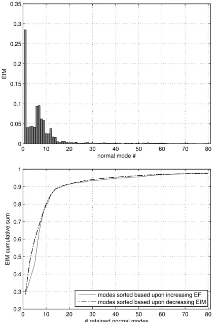
By summing the so-obtained values, a measure of dynamic completeness of a reduced representation in which Nknormal modes are retained is given by:

˜ Ek= Nk ∑ i=1 Ei (3.16)

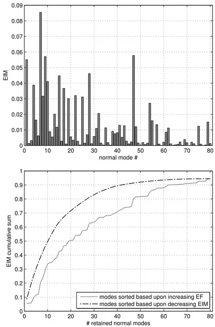
This provides a very useful guideline for mode selection: in fact, one can set a required level of dynamic completeness for the reduced model by simply specifying a threshold value for the EIM cumulative sum (3.16); this implicitly defines how many normal modes, and possibly which ones, should be retained, thus completing the CB mode set selection procedure.

(41)

Theoretical background ₂₉

In addition, a normalized EIM distribution matrix [54], representing the contribution of each fixed-interface mode to the loads at each interface DOF, can be computed as:

E = P2_{[I Diag (M)]}−1

(3.17)

Here, P2indicates a term-by-term square of the modal participation factor matrix, while the Diag operator returns a column vector holding the diagonal elements of the argument matrix: the term in square brackets actually represents the inverse of the diagonal matrix containing the terms from the diagonal of M.

3.1.3 The Modal Truncation Augmentation technique

In this section, a brief explanation is provided about the application of the Modal Truncation Augmentation (MTA) technique to the CB reduction method [23, 31].

Let’s first recall the fixed-interface eigenvalue problem mentioned in (3.5):

Kooϕ = Mooϕ Ω (3.18)

When normal modes are mass-normalized, the flexibility matrix associated to the structure interior can be expressed as:

G = K−1oo= ϕ Ω−1ϕT (3.19)

Since not all modes are retained in the reduced component representation, the complete modal basis can be divided into kept modes (subscript k) and deleted, or truncated, modes (subscript d). Equation (3.19) can thus be expressed as:

G = Gk+ Gd= ϕkΩ−1k ϕTk+ ϕdΩ−1d ϕdT (3.20)

The portion of the flexibility matrix not represented by the kept modes is called the residual flexibility matrix; combining (3.18, 3.19, 3.20) that can be obtained as:

Gd = G − Gk= K−1oo(I − MooϕkϕTk) (3.21)

Let’s now consider the CB transformation equation (3.3). The interior ac-celerations are simply obtained by taking the second time derivative of the corresponding displacements:

¨

(42)

Using (3.8) this can be expressed as:

¨

uo= ψ ¨ua+ ϕ_kP ¨ua− ϕ_kΩkqk (3.23)

Going back to the equation of motion in physical coordinates as expressed in (3.2), considering the second row partition and solving for the interior-DOF displacements one obtains:

uo= − K−1oo(Moau¨a+ Moou¨o+ Koaua) (3.24)

Substituting (3.23) into (3.24) and using (3.7c, 3.21) gives after some simple ma-nipulation:

uo= ψ ua+ ϕkqk+ χ ¨ua (3.25)

where the matrix χ is a matrix of static displacement vectors associated with the internal inertia loads due to unit accelerations at each interface DOF while keeping the other interface DOFs constrained:

χ = −Gd(Mooψ + Moa) (3.26)

These vectors are finally orthogonalized with respect to the interior mass and stiffness matrices by solving an eigenvalue problem:

K_χµ = Mχµ Λ (3.27)

where Mχand Kχare computed ahead as:

M_χ= χT_M

ooχ (3.28a)

K_χ_{= χ}TK

ooχ (3.28b)

The matrix holding the Modal Truncation Vectors (MTV) can now be defined:

γ = χ µ (3.29)

If mass normalization is enforced for the eigenvectors µ in (3.27), then the following holds:

γT_M

ooγ = µTχTMooχ µ = µTM_χµ = I (3.30a)

γTK

ooγ = µTχTKooχ µ = µTK_χµ = Λ (3.30b)

The MTVs in γ can then be depicted as pseudo-eigenvectors associated with the squared pseudo-eigenfrequencies in Λ. They are consistent with the mass-normalized eigenmodes in ϕk, cfr. (3.18), and orthogonal to those with respect

(43)

Model reduction implementation ₃₁

to the interior mass and stiffness matrices, being related to the deleted modes ϕd:

they can thus be regarded as high-frequency fixed-interface correction modes. The augmented CB coordinate transformation can then be written as:

{ua uo} = [ I 0 0 ψ ϕk γ] ⎧⎪⎪⎪ ⎨⎪⎪ ⎪⎩ ua qk q_γ ⎫⎪⎪⎪ ⎬⎪⎪ ⎪⎭ (3.31)

Note that, while the size of the problem has increased by the number of additional modal coordinates q_γ, its topology is completely unaltered, cfr. (3.3): that makes the method quite appealing, since the only additional effort is represented by the computation of the truncated displacement vector matrix χ, according to (3.26), and the subsequent solving of the eigenvalue problem in (3.27). Concerning the latter, it is worth clarifying that the number of MTVs is, in general, equal to the number of the interface DOFs defined for the structure: usually, especially in multibody dynamics applications, these are much fewer than the interior DOFs, so that solving the problem defined in (3.27) normally requires a small computational effort when compared to the eigenproblem related to the structure interior, cf. (3.18).

3.2 Model reduction implementation

3.2.1 Preprocessing

Finite Element models of the crankshaft and the connecting rod have been produced first, these representing the major components in the system. Since Nastran has been employed as FE software, Nastran terminology will be used in the following.

In both cases, the geometry has been simplified at the beginning of the process by removing all those features, as small fillets, which do not contribute significantly to the dynamic behaviour of the components, in order to make the meshing process as simple as possible and to speed up the modal reduction phase, by limiting the involved number of elements. Such a step is crucial when several modal reduction alternatives need to be investigated, as in the present research work, but should be avoided whenever the objective of the multibody modelling activity is to evaluate stresses on the components: in fact, this could be performed soon after the nonlinear simulation stage on the same component models by using modal-based stress recovery methodologies.

Second order tetrahedral elements (TET10) have been used for meshing purposes, those leading to better stiffness estimation with respect to their first order counterparts (TET4).

(44)

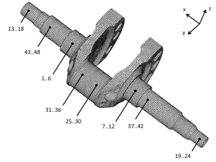
Figure 3.1 Crankshaft FE model. Interface DOF numbering is evidenced.

Particular care has been taken in the definition of interface DOFs. As dis-cussed, in the CB technique a constraint mode is added to the reduced model representation for each of those DOFs: if all DOFs associated to all nodes lying on the interface surfaces of the considered component were placed in the a-set, then the dimension of the reduced solution would become unsuitable for non-linear simulation purposes. Some sort of interface reduction is then required in order to minimize the total number of constraint modes. A common solution to this problem is based on the definition of condensation nodes, whose DOFs are placed in the a-set, which are linked to their corresponding interface surface nodes by means of multipoint constraint elements. Two kind of such elements are available in Nastran: RBE2 are rigid multipoint constraints which connect the interface surface nodes to the condensation node such that they are constrained to move as a rigid system, while RBE3 are interpolation multipoint constraints which define the displacement and the rotation of the condensation node as a weighted average of the motion of the interface surface nodes. Whereas RBE2, introducing artificial numerical stiffness, might result in an overestimation of the stiffness associated to the interface boundary conditions, RBE3 might lead to an underestimation, since interface surface deformation is permitted: the analyst is then required to properly choose between the two based upon the nature of

(45)

Model reduction implementation ₃₃

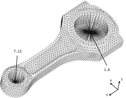
Figure 3.2 Connecting rod FE model. Interface DOF numbering is evidenced.

the various interfaces in the system.

In the present work, a total of eight condensation nodes were defined for the crankshaft, while two were identified for the connecting rod, see Figures 3.1, 3.2. RBE2 were used at the main bearing interfaces, since the crankshaft is somehow stiffened at those locations by the presence of the ball bearing inner rings. RBE2 were also used at the interfaces between the crankshaft and the two pinions, as well as at the crankshaft-flywheel interface, since pre-stressed contacts increase the stiffness at those locations1. On the other hand, RBE3 were adopted at the big end and small end interfaces, both on the crankshaft and on the conrod, since the clearance there allows considering the interface surfaces to deform almost independently from each other.

In each case, the condensation node has been placed at the center of the cor-responding interface surface. For RBE3, the user is required to provide weighting factors for each interface surface node, which should be proportional to the part of the interface surface represented by each of those nodes. In order to avoid this time-consuming and mistake-prone activity, the interface surfaces have been meshed regularly, so that a unitary weighting factor can simply be assigned to

1

Such behaviour has been evidenced by performing experimental modal analysis on a simi-lar crankshaft, in several configurations, and by comparing the results with the corresponding numerical ones.