Within-between decomposition of the Gini index: a novel proposal

Within-between decomposition

of the Gini index: a novel proposal

Federico Attili

Quaderni - Working Paper DSE N°1153

Federico Attili

*

July 23, 2020

Abstract

The socioeconomic impact of spatial concentration has been receiving an increasing attention dur-ing the last two decades. Consequently, the necessity of effective measures of this phenomenon has increased too. This paper considers a population partitioned by subgroups and develops a decomposition of the Gini index in two components, which measure the within and the between group inequality and are also particularly effective to quantify spatial concentration. Indeed, they possess a crucial property which overcomes important issues that may arise using any Gini index decomposition in the spatial context, following a recent approach. In addition, the availability of an only-two highly informative components decomposition provides in numerous applications and several frameworks further significant advantages in the determination of the contributions to global inequality of the intra and the inter groups differences. The ability of the components to capture these phenomena is supported by a parametric bootstrap procedure. This highlights extremely high correlations between the components and two axiomatically derived benchmarks. The presentation of a case study concerning the income distribution in the Italian provinces con-cludes the works, the informativeness and the interpretative advantages of the proposed decom-position appear evidently.

Keywords Inequality decomposition•Gini index•Regional inequality•Spatial concentration

JEL classification: D31; D63; O15; R10; R12

*_{Department of Economics, University of Bologna, Piazza Scaravilli 2, 40126 Bologna, Italy.}

Non technical summary

In the last two decades an increasing attention has been paid to the study of between territories inequality and its socioeconomic impact. Driven by this cutting-edge attention on territorial in-equality and, more in general, on the effects of spatial concentration - which accounts for both inequality and its spatial distribution - a particular new emphasis has to be also devoted to the ability of effectively measuring these phenomena.

Several measures of spatial concentration have been proposed in literature. They can be very useful but they also introduce some kind of arbitrariness. An alternative solution might be to exploit the information nested in the most used inequality measure, following a recent approach. We specifically consider the Gini index and propose a within-between decomposition of the index that nests considerable information on both the inequality and its spatial distribution.

The decomposition proposal deals with partitioned population and only consists of the two in-tra and inter groups inequality. The availability of an only-two highly informative components provides relevant advantages in a descriptive context or a regression task in terms of both in-terpretability and parsimony. To our knowledge, this is the first attempt of decomposition of the Gini index dealing with a partitioned population which comes up with just two components. We also notice that all the well known subgroup decompositions of the Gini index possess three components and a between component that only accounts for the variability of the means of the groups. This may be an oversimplification when the interest lies on the overall distance between distributions. Thanks to a crucial property, the between component from our proposal solves this potential drawback and further issues that may arise employing any Gini index decomposition in the spatial context.

We demonstrate that both the components are highly informative thanks to their properties and because - as we support by employing a parametric bootstrap procedure - they strongly and positively correlate with their relative benchmark. The two benchmarks which have been con-sidered are developed ex ante to reach their objective - to measure the within and the between inequality - without constraining their sum to a preassigned formula, such as in our case with reference to the Gini index. They are derived from literature and follow an axiomatic approach. Hence, the introduced components approximately provide all the information contained in the benchmarks and observe their axiomatically derived properties, despite the fact that they are de-rived with a decomposition boundary - and not independently as for the benchmarks.

In addition, we prove that the same levels of correlation also hold in a real data analysis. We apply the proposed decomposition to the municipality based Income and principal Irpef variables statistical data, which are available on the Open-Source Data released by the Department of Fi-nance of the Italian Ministry of Economy and FiFi-nance. In the bootstrap procedure the correlation values are calculated simulating from independent scenarios. In the real data analysis we comple-ment the assesscomple-ment calculating correlations over time - our analysis ranges from 2000 to 2017 - and over different territorial aggregation. This strengthens the already mentioned results on the informativeness of the components.

With the same data - focusing on the income distribution of the Italian provinces - we also high-light the advantages of the proposed between component share in assessing the spatial distribution of inequality and the interpretative benefits that a two-component decomposition ensures in em-pirical contexts.

In fact, the decomposition is inspired by the spatial framework. Nonetheless, several appli-cations of our decomposition are also meaningful and convenient outside of this context: groups could be defined by several factors such as gender, education level, occupation, race, age, or other criteria.

1 Introduction

Inequality between territories of the same country has been diffusely considered as just ancil-lary in the analysis of the inequality for a long period. But the presence in several countries of many territories which have been left behind is leading to increasing socioeconomic problems and facilitates populism, as Rodr´ıguez-Pose (2018) pointed out. An increasing attention has been recently paid to the study of place-based policies (see e.g. Neumark and Simpson,2015; Kline and Moretti,2014). Driven by this cutting-edge attention on the territorial inequality and, more in general, on the effects of spatial concentration - it accounts for both inequality and its spatial distribution - a particular new emphasis has to be also devoted to the ability of measuring these phenomena.

The inequality indexes such as the Gini or the Theil index (only to mention the most used) are invariant to permutations of the units in the space. This can lead to the same inequality value associated to drastically different spatial patterns of the variable of interest - in this paper we will refer to income - as Arbia (2001) and Arbia and Piras (2009) effectively clarified. This means that the classical inequality measures can not be used to assess spatial concentration because they only partially capture this phenomenon. A symmetric argument holds for the spatial autocorre-lation measures (see e.g. Moran,1950; Ord and Getis,1995), which only deal with the income distribution along space but do not capture concentration.

Several measures of spatial concentration have been proposed in literature, see among the others Ellison and Glaeser (1997), Campante and Do (2007), Bickenbach and Bode (2008) and Arbia and Piras (2009). They can be very useful but they introduce some kind of arbitrariness: in Ellison and Glaeser (1997) and Bickenbach and Bode (2008) the choice of a reference distribution is required; the proposal introduced in Campante and Do (2007) defines a centered index of spa-tial concentration and is appropriate when there is a place that can be considered central w.r.t. the others; in Arbia and Piras (2009) a class of measures of spatial concentration which depend on the choice of a spatial autocorrelation statistic is developed.

An alternative solution might be to combine inequality and spatial autocorrelation measures, as firstly suggested in Arbia (2001). The introduced proposal was criticized in Bickenbach and Bode (2008) which considers it as an ad hoc measure, but a similar approach was also adopted in A. Shorrocks and Wan (2005). Here, the authors suggest to exploit a subgroup decomposition of an inequality index in the spatial context. This means partitioning the population into geograph-ical regions and evaluating a within component that measures the intra-territories inequality by a weighted average of the inequality index in each region; and a between term that measures the variation in the means of the regions. The idea of Shorrocks and Wan consists in assessing the distributional impact of spatial factors by jointly considering the overall inequality and the share of the between component. In this manner both the inequality and its spatial distribution - the key features of spatial concentration - should be under control. Rey and Smith (2013) also pursued a similar idea. They specifically consider the Gini index and propose a within-between decomposition of the index arguing that it potentially nests sufficient information on both the in-equality and its spatial distribution. The main diversities between the two approaches are that the decomposition in Rey and Smith is not a subgroup decomposition and does not require a parti-tion of the populaparti-tion. Rey and Smith have decomposed the index according to a matrix which defines pairs of neighbours and non-neighbours. The differences between the former constitute the within component while the latter sum up to the between term. More on the properties of the two strategies will be discussed in the following section.

In this paper we follow these recent approaches and introduce a novel proposal to decompose the Gini index. It deals with partitioned population and only consists of two components - within and between - which result to be highly informative on the intra and the inter groups inequality. To our knowledge, this is the first attempt of decomposition of the Gini index dealing with a par-titioned population which comes up with just two components. We will show that its properties guarantee important benefits and makes it also particularly effective to measure spatial

concen-tration, in the spirit of Arbia (2001), A. Shorrocks and Wan (2005) and Rey and Smith (2013). In fact, the work is inspired by the spatial framework that is clearly considered throughout the work - the groups could be the regions or the sub-regions in a country, or the countries in a confederation - and we often refer to any within-between decomposition as to a spatial decompo-sition; and to the within and the between terms as to its spatial components. Nonetheless, several applications of our decomposition are also meaningful and convenient outside of this context: groups could be defined by several factors such as gender, education level, occupation, race, age, or other criteria.

In Section 2 we present the main features of the most common decompositions of the Gini index. Then we discuss the possibility of a two-component decomposition dealing with parti-tioned population to exist; and its potential advantages. Section 3 introduces our decomposition methodology when the groups are equal-sized and explains its ratio; a crucial property of the obtained components is also derived. Section 4 generalises the procedure to the different-sized groups case. In presenting Section 5 we stress how a rigorous axiomatic approach was followed to accept an index as an inequality measure (see Allison,1978for an effective overview). We be-lieve the same approach should also be pursued when evaluating the components of an inequality index decomposition. Thus Section 5 shows, by employing a parametric bootstrap procedure, that the components strongly and positively correlate with two related benchmarks. They are inspired by literature and axiomatically derived to measure the within and the between inequality. Section 6 proves that the same levels of correlation also hold in a real data analysis, strengthening the preceding section results on the informativeness of the components; it also highlights the advan-tages of the proposed between component share in assessing the spatial distribution of inequality and the interpretative benefits that a two-component decomposition ensures in empirical contexts. Section 7 gives conclusive remarks.

2 Decomposing the Gini index

A very comprehensive outline of the most common subgroup Gini index decompositions (Bhat-tacharya and Mahalanobis,1967; Rao,1969; Pyatt,1976; Mookherjee and A. Shorrocks,1982; Yitzhaki and Lerman, 1991; Dagum, 1997) is provided in Radaelli (2010). These proposals are developed by different approaches but the resulting components - except the ones derived in Yitzhaki and Lerman (1991) - coincide. They all rely on a population of N individuals which is partitioned in K groups; and exhibit three components: the two spatial components and a third term.

The within components measure the intra-territories inequality by a weighted average of the Gini index in each group, where the weights vary with the considered decomposition. Let Gk be the

value of the Gini index in group k = 1,...,K; µk and nk its mean and dimension;µ the overall

mean. In the within component from Yitzhaki and Lerman (1991):

GY L w = K

Â

k=1 ⇣ nk N ⌘✓ µk µ ◆ Gk= K

Â

k=1 skGk (1)

each weight sk is immediately interpretable as the income share of the group k. In the other

proposals - we will refer to them considering their first specification from Bhattacharya and Ma-halanobis (1967) - the income shares are multiplied again by the population shares:

GBM w = K

Â

k=1 ⇣ nk N ⌘2✓ µ_k µ ◆ Gk= K

Â

k=1 ⇣ nk N ⌘ skGk (2)

The between component also depends on the decomposition choice, but every proposal presents a measure which substantially just compares the means of the groups. As for the two decomposi-tions we are considering, they are:

GY Lb =_µ2Cov µk, 1 nk n_k i=1Rik N ! (3) where Rikis the rank of the unit i from the group k in the overall population; and

GBMb =_2µ1 K

Â

k=1 K

Â

h=1 nknh N2 |µk µh| (4)

The two components in eq. (3)-(4) appear very different in their form but they account accordingly for low levels of territorial inequality when the groups have similar means - they are zero if the means are identical - and vice versa, regardless of the potential different dispersion within each group. This could be an oversimplification when the overall distance between the distributions is relevant, as Ebert (2010) effectively pointed out.

The third term of the decompositions - which disappears if the group distributions do not over-lap - has been left uninterpreted in the first attempts of decomposition and considered just as the residual which guarantees the identity. Then several interesting interpretations in terms of groups overlapping or stratification have been proposed (Yitzhaki and Lerman, 1991, Yitzhaki, 1994) and all the three components became potentially useful and informative.

Nonetheless, it is incontestable that every two-component decomposition possesses an important advantage: all the information of the inequality index and its decomposition can be provided spec-ifying only the overall inequality and its between component. Indeed, the collinearity between the inequality index and the two spatial components allows to provide all the information contained in the decomposition by delivering only two of these three values, with relevant advantages in a descriptive context or a regression task in terms of both interpretability and parsimony. The num-ber and the specification of the components may become relevant also when measuring spatial concentration using an inequality index and the share of its between component, as will become clear in Section 6.

These arguments and the potential oversimplification generated by a between component relying only on the means of the groups encouraged us to look for a novel solution. As we will show, this possesses both the advantage of a two-component decomposition and a between component which informs about the differences between the overall group distributions.

Actually, the spatial Gini index decomposition presented in Rey and Smith (2013) is also com-posed only by the two spatial components and its between component directly relies on the indi-vidual values - not only on the means. However it is only appropriate when the population groups do not form a partition. When they do, a relevant drawback arises: the between component is pos-itive even if the groups have the same distribution, hence it may tend to overestimate the between group inequality in cases of groups characterised by similar distributions.

As we have anticipated, in this paper we introduce the first two-component decomposition of the Gini index dealing with a partitioned population. This could appear in contrast with the well known results presented in Bourguignon (1979), A. F. Shorrocks (1980) and A. F. Shorrocks (1984) where the class and the properties of the measures which are additively decomposable are derived. The Gini index is not additevely decomposable in the sense intended by these works, which is partitioning the population into geographical regions and expressing the index as a weighted average of the inequality values within each group, plus some contribution arising from the variation in the means of the regions. Such a decomposition on the Gini index requires a third component, as we explained above.

Differently, our proposal determines a between component which does not rely on the means of the groups but directly depends on the incomes of individuals. This allows a two terms decom-position to exist and to perform better than the other decomdecom-position proposals when the groups overlap1_{. In addition, as we will show in the following section, the between term is null if and only}

(a) Couple differences composing g (b) Decomposition in the non-trivial case

Figure 1: A two-group-two-individual illustration

if the groups have the same distribution. The sufficiency of this condition solves the drawback of the decomposition in Rey and Smith (2013) while its necessity solves the oversimplification of a between component substantially relying just on the means of the groups.

3 The decomposition proposal

Keep on considering a population of N individuals. Let xibe the income of the generic individual

i = 1,...,N. The Gini index is defined as follows:

G =_2µN1 ₂

Â

N i=1 N

Â

j=1 xi xj =_2µNg ₂ whereµ = 1

NÂN1xiis still the average income. The index accounts for the sum g of all the

dif-ferences between individual incomes, averaging and normalizing by the factor 2µN2 1_{, so that}

G is scale invariant and G 2 [0,1] if all the xi 0. Consider now the population partitioned in K

equal-sized groups, i.e. nk=n 8 k = 1,...,K and define xki to be the i-th element in the ordered

vectorxk_{= (x}k

1, . . . ,xkn)with xki xki+1 8 i = 1,...,n 1. All the information concerning with

the spatial distribution of inequality is within g, which can be reformulated as

g =

Â

K k=1 K

Â

h=1 n

Â

i=1 n

Â

j=1 xk i xhj (5)

The assumption of equal-sized groups might be thought as extremely simplistic but, as we will show in Section 4, it is only apparently limiting in the applicability of the proposal. Conversely, it provides a deeply innovative insight into the structure of the Gini index.

Look at the Figure 1 which shows a two-group-two-individual situation. Figure 1a highlights the absolute differences between all the couples of units, considered twice so that they consti-tute g if they are summed up. As the scheme suggests we distinguish three kind of differences: vertical, horizontal and diagonal ones. The vertical differences compare same-group pairs of ele-ments. The horizontal differences compare same-rank pairs from different groups. The diagonal differences compare different-rank pairs from different groups.

As a point of departure, we would like a decomposition which assigns the vertical and the horizontal absolute differences to the within and the between component, respectively.

Despite the fact that the diagonal differences involve different-group pairs, they partly reflect the vertical differences - i.e. the within inequality - and can not be totally addressed to the between group inequality. Consider a situation with two identical groups: the possibly positive values of the diagonal differences equal the vertical ones and can not be addressed to the absent between group inequality.

In Lambert and Aronson (1993) the residual term is described as “at once a between groups and a within groups effect: it measures a between groups phenomenon, overlapping, that is generated by inequality within groups” (p. 1224). The sum of the diagonal differences especially accom-modates this characterisation and can be thought as a kind of residual term of this decomposition strategy. In fact, this term is unambiguously dependent on the interaction of the intra and the inter groups differences but it does not disappear when the groups do not overlap. Thus it can not be interpreted as an overlapping component.

This is not an issue for our purpose because with the equal-sized group representation a quite intuitive and effective paradigm to decompose the diagonal differences exists and generates two contributes to the spatial components.

Sometimes, an extremely reasonable strategy is viable to decompose the diagonal lines and to disentangle the within contribution from the different-group differences. We invite the reader to inspect the diagonal differences and to move along the legs of the triangles depicted in the scheme in Figure 1a. Look at the solid black diagonal line as an example: the absolute difference between the richest of the group k and the poorest of the group h is 6. The former is 5 units richer than his group poorest individual, who is 1 unit richer than his counterpart in group h. A similar argument holds from the opposite point of view, looking at the difference between the poorest of group h and the richest of group k - dashed black diagonal line. The diagonal absolute differences between the two individuals considered in the example are predominantly due to the within inequality in the two groups and reflect it. Accordingly, we suggest to split the global contribution to g of the couple composed by the richest of the group k and the poorest of the group h (6 + 6 = 12) assigning 5 + 4 = 9 to the within component and 1 + 2 = 3 to the between one.

This straightforward strategy is not directly feasible in situations - such as those represented by the gray lines - in which the three values involved in the path along the legs do not increase or decrease monotonically as in the black lines situations, namely when the product between the horizontal and the vertical difference is negative. In such cases we should subtract the horizontal value from the vertical one to obtain the value of the difference along the diagonal, with paradox-ical effects on interpretation if we subtract the horizontal value - 1 - from the between component. As an example, imagine to replace the poorest individual of group h with a poorer one. We would obtain a lower value of the between inequality (we subtract a value 3 (2 e) > 1) even though the intuition suggests the between inequality is now higher - the poor group is poorer - and we should sum up a positive value to it.

To overcome this problem, we propose to reduce both the vertical and the horizontal values pro-portionally to make their sum equal to the diagonal difference. Hence, both the vertical and the horizontal values are divided by their sum and multiplied by the diagonal difference - look at the Figure 1b for an illustration. In other words we suggest to split each diagonal difference proportionally to the vertical and the horizontal ones and to assign these two (positive) values to the within and the between component, respectively. Thanks to this solution we preserve both reasonable proportions between the values added to the spatial components - these proportions observe the black lines decomposition argument - and the Gini index compliance, i.e. the pos-sibility to have a two-components decomposition. With this overall strategy the contributions of the diagonal differences to the within and between inequality mimic to the utmost the vertical and horizontal differences. This is the key that makes the two components highly informative. Until now, we have just presented the intuition at the base of the decomposition. We will now generalise this strategy, formalise the decomposition proposal and deliver the two spatial compo-nents. At the end of this section, the preannounced property of the two components is derived. For each difference |xk

and their product c = (xk i xkj)(xkj xhj). We can write: xk i xhj = xki xhj xk i xkj + xkj xhj xk i xkj + xkj xhj = xk i xhj xk i xkj Lkh i j + xk i xhj xk j xhj Lkh i j = = 8 > > > < > > > : xk i xkj + xkj xhj if c 0 xk i xkj |x k i xhj| Lkh i j + xkj xhj |x k i xhj| Lkh i j if c < 0 (6)

where to obtain the first equation we exploited the fact that c 0 implies |xk

i xhj| = |xki xkj+

xk

j xhj| = Lkhi j.

We propose to assign the first and the second addends of eq. (6) to the within and the between inequality components, respectively. The first equation fills all the trivial-case decompositions (the vertical differences when k = h; the horizontal differences when i = j and the black diagonal differences kind when k 6= h and i 6= j) while the second stands for analogous situations to the two sketched by the gray lines.

We stress here the importance of the equal-sized groups hypothesis which guarantees that each unit has a counterpart in each other group, i.e. given the couple (xk

i,xhj), the element xkjalways

exists. Notice that considering xk

jor xhi in the decomposition is not an issue, since the Gini index

counts each difference twice by inverting the indices of the summations. To simplify the notation in eq. (6) we define2_wkh

i j =|x k i xhj| Lkh i j and obtain: xki xhj = xki xkj wkhi j+ xkj xhj wkhi j (7) It is always wkh

i j 2 [0,1]: wkhi j 0 holds by definition and wkhi j =1 iff c 0. Hence, |xki xkj|wkhi j

and |xk

j xhj|wkhi j can be considered, respectively, as the contributions of the difference |xki xhj| to

the within and the between group inequality; and wkh

i j the vertical and the horizontal differences

rescaling factor. This factor can be less than one because of the possibility of a proportional reduc-tion of the horizontal and the vertical values before assigning them to the spatial components: as we showed in the numerical example, the difference |xk

i xhj| can be less than |xki xkj| + |xkj xhj|

(it happens iff c < 0), so we have to rescale the two addenda by the factor wkh

i j  1. This value

de-creases, by definition, according to the ratio between the diagonal difference and the summation between the horizontal and the vertical ones. This means that when two individuals are similar the contribution of their couple to the within and the between components are accordingly small, even if the two vertical and horizontal differences involved in the decomposition are greater. The latters account, as desired, only in the proportion between the two spatial contributions, while their absolute values depend on the starting level of the inequality in the couple.

The Gini index decomposition proposal can be now derived just by substituting eq. (7) into eq. (5). DenotingÂK

h=1wkhi j =wki jandÂni=1wkhi j =wkhj , we have:

g =

Â

n i=1 n

Â

j=1 K

Â

k=1 xk i xkj wki j+ K

Â

k=1 K

Â

h=1 n

Â

j=1 xk j xhj wkhj =gw+gb (8) and G = Gw+Gb=_2µNgw₂+_2µNgb₂

The Gini index appears composed by only two terms. We propose to interpret the first as the

2_{We set w}kh

within component of the inequality, because it depends on the summation of the contribution of all the couples of units belonging to the same group, i.e. the couple differences multiplied by the relative weights wk

i j; and the second as the between component of inequality, because it depends

on the summation of the contribution of all the couples of same-rank units in different groups, i.e. the couple differences multiplied by the relative weights wkh

j .

Note that the within and the between component involve, respectively, the weights wk

i j and wkhj

which do not exclusively depend on the differences within or between groups. This is not a drawback but a necessary property which allows each contribute of the intra-group (same-rank units) differences to the within (between) inequality to depend on how it affects the different-rank units differences, i.e. the diagonal ones. Indeed wk

i j(wkhj ) grows when the diagonal differences

are enlarged by the vertical (horizontal) ones. Given that wkk

i j =1, wkhj j=1 and wkhi j 0 8i, j,k,h imply wki j 1 8k,i, j and wkhj 1 8 j,k,h,

the crucial property - that we have mentioned before - of the two spatial components is ensured: Gw=0 () |xki xkj| = 0 8 i, j,k

Gb =0 () |xkj xhj| = 0 8 j,k,h

The first relation ensures the within component to be zero iff all the intra-group differences are zero, i.e. all the individuals equal their group mean. Actually, all the decompositions we have considered until now possess this property. The second relation is symmetric to the first and guarantees the between component to be zero iff all the same-rank differences are zero, i.e. all the groups have the same distribution. This is a very reasonable condition too - at the end of the previous section we have already stressed the relevant advantages it ensures - but it is satisfied just by our component.

As stressed before, the structure of the weights wk

i jand wkhj depends on many units and not only

on the two involved in the difference they multiply. Unfortunately, this compromises the analyti-cal tractability of the expressions we obtained for the two components and hinders the derivation of additional properties. An alternative approach to corroborate the appropriateness of the two components is followed. Section 5 will show that each component strongly and positively corre-lates with a related benchmark. The two benchmarks which have been considered are developed ex ante to reach their objective - to measure the within and the between inequality - without con-straining their sum to a preassigned formula, such as in our case with reference to the Gini index. They are derived from literature and follow an axiomatic approach.

We have essentially demonstrated that the two components have a correct starting point - zero - and we will demonstrate that they move in the right direction and proportion with reference to different scenarios, because they strongly correlate with their relative benchmark. These two properties have a remarkable consequence: the components approximately provide all the infor-mation contained in the related benchmarks and observe their axiomatically derived properties. In addition, the extent of the approximations is small because it inversely depends on the (high) correlation values.

In the following section we show that the equal sized groups hypothesis is not binding. It is necessary to understand the decomposition arguments but the proposal can be easily generalised to cope with a more realistic situation in which groups have different sizes.

4 Different-sized groups

Consider now the K groups having a vector of sizesn = (n1, . . .nK)whereÂKk=1nk=N. We have:

g =

Â

N i=1 N

Â

j=1 xi xj = K

Â

k=1 K

Â

h=1 nk

Â

i=1 nh

Â

j=1 xk i xhj

Figure 3: Exact approach: a two-group illustration

and a way to guarantee the element xk

jto exist is needed to employ the decomposition proposal.

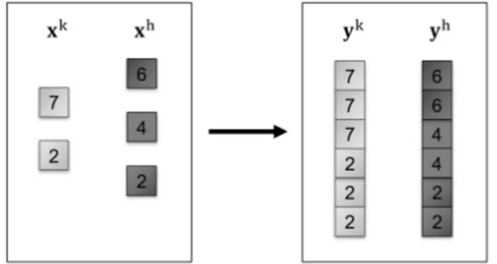
We can proceed by two distinct approaches. The first allows to evaluate with no approxi-mation the two components but necessitates potentially unaffordable computations. The second drastically reduces computational requirements paying the cost of a negligible approximation. The exact approach. It exploits the principle of population. It considers a new common size n = mcm(n) and the resampling weights pk= nnk so to build the vectors yk = (yk1, . . . ,ykn) =

(xk 1. . .xk1 | {z } p_k1 , . . .xk n_k. . .xkn_k | {z } p 1 k ). Defining li m_k =pk1(i 1) + mk, by construction we have xki =ykli mk,

8 i = 1,...nkand 8 mk=1,..., pk1. Hence 8 (k,h) 2 {1,...,K}⇥{1,...,K} the following holds:

nk

Â

i=1 nh

Â

j=1 xk i xhj = n

Â

i=1 n

Â

j=1 pkph yki yhj (9) Proof. n

Â

i=1 n

Â

j=1 pkph yki yhj = n_k

Â

i=1 n_h

Â

j=1 p 1 k

Â

mk=1 p 1 h

Â

mh=1 pkph yk_li mk y h l_mhj = n_k

Â

i=1 n_h

Â

j=1 p 1 k

Â

mk=1 p 1 h

Â

mh=1 pkph xki xhj = = nk

Â

i=1 nh

Â

j=1 pkphpk1ph1 xki xhj = nk

Â

i=1 nh

Â

j=1 xki xhj

Substantially, imagine to have two groups composed, respectively, of two and three individu-als, as the ones reported in the left rectangle of Figure 3, and replace them with those in the right part. By the principle of populationxk_andyk_{(as well asx}h_andyh_{) are identical from the point of}

view of their internal inequality, and also the comparison between the two groups should remain unvaried. Notice that each difference in the left scheme appears in the right scheme nine times if the couple belongs toyk_{, four times if it belongs toy}h_{and six times if the units belong to different}

groups. In order to respect the principle of population we have only to adjust for this effect. This is what eq. (9) means.

The Gini index numerator can be now decomposed with an analogous technique to the one em-ployed deriving eq. (8). The following is obtained:

g =

Â

N i=1 N

Â

j=1 xi xj = K

Â

k=1 K

Â

h=1 nk

Â

i=1 nh

Â

j=1 xk i xhj = K

Â

k=1 K

Â

h=1 n

Â

i=1 n

Â

j=1 pkph yki yhj = = n

Â

i=1 n

Â

j=1 K

Â

k=1 yki ykj wki j+ K

Â

k=1 K

Â

h=1 n

Â

j=1 ykj yhj wkhj =gw+gb (10)

The only difference w.r.t. eq. (8) is in the new weights wk

i j=ÂKh=1pkphwkhi j and wkhj =Âni=1pkphwkhi j.

They are the general case of the previous defined weights and incorporate the information needed to preserve the original impact of each couple.

As we said, in most cases this approach requires an unaffordable computational effort because of the potentially huge magnitude of the minimum common multiple. Thus, we present an alter-native procedure which drastically reduces computational requirements paying the minimal cost of a negligible approximation.

Quantilisation. We propose to replace the vectors yk_{with others K vectors: for each group we}

se-lect a vector composed by n quantiles from the income vector of the group. As for the resampling weights, their calculation is the same employed in the exact approach, but now nothing ensures n nkso it can be pk>1. The decomposition proposal has the same form of eq. (10) but G, Gw

and Gbnow incur in some approximation.

In order to employ this method there are the definition of quantile and the value of n to be selected.

As for the former, we advise the definition 7 reported in Hyndman and Fan (1996), which is also the default definition adopted by the quantile() function in the software R. Given each vector xk

2 Rnk, accordingly to this definition and in order to alter as little as possible the

quantilisa-tion results w.r.t. the exact calculaquantilisa-tion, we suggest to interpolate linearly the vertices⇣ i 1

nk 1,x

k i

⌘ where i = 1,...,nk, and then to estimate the n quantiles by determining the values associated to

the probabilities

probj=_{n 1}j 1 j = 1,...,n (11)

on the resulting piecewise linear curve. As for the latter, we define wk=_ÂKnk

k=1nk and recommend the value

n =

Â

K k=1 wknk=Â K k=1n2k ÂK k=1nk (12)

This expression determines n as the average of the nk, each weighted by its own share of

popula-tion wk.

A formal assessment which legitimises the decisions proposed both for the quantile definition and for the value of n is provided in the appendix. Here we only inform about the negligibility of the approximation which the quantilisation procedure cope with when the advised definitions are employed.

Actually, the optimal performance associated to these two decisions should not come as a surprise. The outstanding results of the proposed choice of n derives directly from the consistency with the resampling weights system. This choice assigns greater weights wkto the sizes of the most sized

groups, which is desirable because these are the groups the biggest values of pk are associated

to. It is reasonable to preserve their information choosing a large n and resampling the smaller groups. But if many small groups are present n is attracted towards their small size. Here the quantilisation reduction of big groups and the related loss of information are preferred to pay the approximation cost of the quantilisation resampling for many small groups. Nonetheless, notice that it could be also acceptable to choose a value n << min(n) if min(n) is high and a computational cost saving choice is required.

With the choice determined by eq. (11) the values pj partition the interval [0,1] in n 1 equal

parts, with 0 and 1 two of the n vertices of the partition. It is straightforward to verify that, also employing the quantile selection procedure discussed, min(xk_{)and max(x}k_{)are preserved for}

each n and k. Moreover, if n = nkfor any k the vectorsxkare entirely preserved, too. Both this

properties hold at the same time only employing the definition 7 and the discussed choice of the values pj. They ensure robustness to the quantilisation procedure w.r.t. outliers and contribute to

explain the negligible approximation incurred.

We finally observe that a generalised version of the quantilisation procedure may be wanted to increase its appropriateness in coping with weighted data, i.e. to consider the weights of the observations. We suggest - but other choices we do not discuss here can be also suitable - to employ functions which account for the sample weights in returning quantiles (as the R function wtd.quantile()) in place of a standard quantile function (as the R function quantile()). This is equivalent to applying a stantard quantile function to vectors with the income of each unit in the starting vector repeated as many times as the value of its weight states. We consequently advise to consider the weights summation in each group as the group weight in eq. (12), in place of the defined wk. This is the way we will proceed in Section 6.

In the analysis which follows each group k will be replaced by the n quantiles selected from xk_{. The value of n will be determined by eq. (12). The definition 7 and eq. (11) will be employed}

to select the n quantiles.

In the next section a parametric bootstrap will exhibit that each component of the introduced decomposition strongly and positively correlates with the related benchmark. These results will be compared to the one achieved by employing the components from eq. (1)-(4) in place of the introduced ones. In Section 6 the reliability of the simulation process will be strengthened showing very similar results obtained using real data.

5 Correlation with benchmarks

The two benchmarks which we consider are developed ex ante to measure the within and the between inequality, without constraining their sum to a preassigned formula as it happens for the Gini index decompositions. They are derived from literature and observe an axiomatic approach.

The following equation defines the reference measure of the global intra-group inequality:

Wr= K

Â

k=1

skGk

where Gkis the Gini index in group k and skis the share of income possessed by group k. Hence,

the within benchmark is defined as a weighted average in which the Gini of each group is weighted by its own share of income. Every Gk incorporate the axiomatic approach observed

by the Gini index and the related properties. Thus, the global properties of Wrdepends on them

and on the aggregating consequences of the weighted mean, which in this case assigns a greater weight to the inequality values of the groups which possess the biggest shares of income. This measure coincides with the within component reported in (1). We selected this weighting choice due to its immediate interpretability, as discussed in Section 2.

As for thebetween benchmark, the following index has been selected as the reference mea-sure of the global inter groups inequality:

Br= K

Â

k=1 K

Â

h=1 ⇣ nknh N2 ⌘ Ebkh

where Ebkhis the diversity measure between the two groups k and h proposed in Ebert (1984). He

proposes a class of measures dependent on a parameter r. Here Ebkhis the measure corresponding

to r = 1, which employs the absolute difference as a distance. A slight modification - the incomes are standardized dividing by the average of the populationµ - is required to guarantee the scale invariance criterion to be respected in addition to the other properties the index already observes. The measure is defined as:

Ebkh=_mµ1 m

Â

i=1

0.0 0.2 0.4 0.6 0.8 1.0 0.70 0.75 0.80 0.85 0.90 0.95 1.00 CV(E(xk)) ρ ( Gw , Wr ) A BM YL

(a)Within components.

0.0 0.2 0.4 0.6 0.8 1.0 0.70 0.75 0.80 0.85 0.90 0.95 1.00 CV(E(xk)) ρ ( Gb , Br ) A BM YL (b)Between components.

Figure 4: Correlations between the intra and the inter groups inequality benchmarks and the related spatial components from the three Gini index decompositions: A, YL and BM in the legend stand for the decomposition proposed in this work, in Yitzhaki and Lerman (1991) and in Bhattacharya and Mahalanobis (1967), respectively. The figures report the values obtained simulating with K = 30 andn ⇠ U⇣[100,500]K⌘for different values of CV⇥E⇥¯xk⇤⇤

where m = min(nk,nh) and xki is the i-th of the m quantiles selected from the income vector

of the group k. A preceding proposal by Dagum (1980) had already developed a measure of economic distance but it has been criticized by A. F. Shorrocks (1982) because of its asymmetric nature. Ebert proposal, instead, presents all the properties of a distance and observes a more general axiomatic approach. In addition, it perfectly reflects our idea that a measure of inequality between groups has to compare their overall distributions. Br inherits all these properties and

its value depends on them and on the aggregating consequences of the weighted mean, which in this case assigns greater weights to the inequalities of the couples selected from the groups which possess the biggest shares of couples.

In order to evaluate the extent of the correlation between the components of the three con-sidered decompositions and the related benchmarks, a parametric bootstrap algorithm has been employed. It considers three parameters: the number of groups, the distribution of n and the expected coefficient of variation between the averages of the groups CV⇥E⇥¯xk⇤⇤_.

The algorithm fixes these parameters and generates incomes from a lognormal distribution. Prop-erly, the third parameter is the vector composed by the minimum and the maximum values of the uniform distribution the expected value of the lognormal distribution is drawn from. These two values straightforwardly determine the value of CV⇥E⇥¯xk⇤⇤_{. More details about the income}

simulation procedure and its theoretical foundations can be found in the Appendix. The algorithm evaluates 50 times all the involved indices to estimate the two triples of correlations between the

two spatial components of the three involved decompositions and the related benchmarks. It runs this procedure 20 times and obtains 20 replicates of the following couple of triples of correlation estimates: 2 4cori G A w,Wr cori GY Lw ,Wr cori GBMw ,Wr 3 5; 2 4cori G A b,Br cori GY Lb ,Br cori GBMb ,Br 3 5

with i = 1,...,20. Following the notation introduced in Section 2, the superscripts A, YL and BM identify the decomposition proposed in this work, in Yitzhaki and Lerman (1991) and in Bhattacharya and Mahalanobis (1967), respectively.

Each of the 20 replicates of triples constitute one triple of boxplots in the pertaining diagram reported in Figure 4. The value of CV⇥E⇥¯xk⇤⇤ _{is varied to obtain all the eight triples of}

box-plots. Hence, for each considered value of CV⇥E⇥¯xk⇤⇤_{, the three kinds of boxplots in}

Fig-ure 4a (4b) represent the replicates of the triples: black, gray and white boxplots describe the distribution of the correlation that the within (between) benchmark has, respectively, with the within (between) components proposed in this work, in Yitzhaki and Lerman (1991) and in Bhat-tacharya and Mahalanobis (1967). Figure 4 reports the values obtained simulating with K = 30 andn ⇠ U⇣[100,500]K⌘.

We have varied the value of CV⇥E⇥¯xk⇤⇤_{to evaluate correlations in contexts characterised by}

dif-ferent degree of homogeneity in the vector of the means of the groups. This allows us to notice the evident advantages that the proposed between component has w.r.t. the between components derived from the alternative decompositions - which only account for the variability of the means of the groups - in situations characterised by low and medium levels of variability in the vector of the means of the groups. As for the within component, the one obtained using the decomposition in Yitzhaki and Lerman (1991) presents by definition a perfect correlation with Wr. However,

better than GBM

w , GAwalways reports extremely high correlations with Wr.

Furthermore, the correlation values are studied by the same algorithm in multiple contexts by also varying the number of groups and the distribution ofn. A summary of the results for some representative choices of the parameters is reported in Table 1. It also contains the results already represented in Figure 4. In this table the 20 replicates produced to estimate each correlation dis-tribution are summarised by their averages and standard deviations. These values - obtained from all the eight different levels of CV⇥E⇥¯xk⇤⇤_{- are averaged pairwise determining four values forµ}

and sd. They correspond to low, medium-low, medium-high and high levels of CV⇥E⇥¯xk⇤⇤_.

The results are extremely encouraging. The correlation values of the proposed decomposition only marginally depend on the parameters specification. They just show some negligible vari-ations both in the mean and the standard deviation. We notify the most perceptible. Higher K values negatively influence the within average correlations, but an increase in the values in n seems to absorb this small effect. The within average correlations also decrease for higher level of CV⇥E⇥¯xk⇤⇤_{, while their standard deviations tend to increase. However, the averages are never}

behind 0.92 and the maximum standard deviation is 2.8 · 10 2_{. As for the between correlation, it}

slightly decreases and shows higher standard deviations when the variability inn gets higher and both the values inn and K are small.

Despite all these details, the values of the correlations for the components of the introduced composition reported in Table 1 always maintain analogous advantages to those explained de-scribing Figure 4. The sole exception occurs when the variability inn is small: in this case the results for the within component from eq. (2) are enhanced and turn out to be comparable with the decomposition introduced with this work. Indeed, the former perfectly correlates with the within component from eq. (1) when the groups are equal-sized - it can be easily proved. However, the correlation decreases rapidly as soon as the size variability increases, so this aspect remains a negligible issue. Summarising, Table 1 strengthens the conclusions drawn looking at Figure 4.

W ithin components Between components K = 3 K = 30 K = 3 K = 30 Magnitude of CV ⇥ E ⇥k¯x ⇤⇤ L L-M M-H H L L-M M-H H L L-M M-H H L L-M M-H H n ⇠ U ⇣ [10 ,20 ] K ⌘ µ A 0.972 0.966 0.964 0.961 0.943 0.942 0.944 0.941 0.988 0.986 0.984 0.978 0.990 0.989 0.983 0.977 YL 1.000 1.000 1.000 1.000 1.000 1.000 1.000 1.000 0.386 0.465 0.704 0.807 0.117 0.313 0.468 0.668 BM 0.981 0.977 0.968 0.957 0.963 0.960 0.949 0.932 0.771 0.840 0.903 0.952 0.829 0.881 0.908 0.944 sd A 0.005 0.013 0.010 0.012 0.018 0.016 0.015 0.018 0.006 0.007 0.008 0.006 0.003 0.003 0.005 0.007 YL 0.000 0.000 0.000 0.000 0.000 0.000 0.000 0.000 0.199 0.214 0.131 0.085 0.197 0.215 0.202 0.100 BM 0.013 0.017 0.024 0.031 0.013 0.012 0.018 0.029 0.073 0.050 0.053 0.019 0.060 0.050 0.037 0.015 n ⇠ U ⇣ [10 ,50 ] K ⌘ µ A 0.974 0.970 0.959 0.943 0.946 0.945 0.936 0.921 0.964 0.966 0.965 0.972 0.984 0.982 0.976 0.972 YL 1.000 1.000 1.000 1.000 1.000 1.000 1.000 1.000 0.238 0.445 0.692 0.851 0.033 0.234 0.475 0.734 BM 0.939 0.923 0.899 0.841 0.937 0.925 0.894 0.857 0.683 0.766 0.881 0.943 0.737 0.796 0.891 0.937 sd A 0.009 0.010 0.012 0.020 0.012 0.018 0.020 0.028 0.028 0.031 0.030 0.025 0.006 0.006 0.008 0.009 YL 0.000 0.000 0.000 0.000 0.000 0.000 0.000 0.000 0.249 0.180 0.137 0.066 0.162 0.241 0.232 0.138 BM 0.034 0.043 0.052 0.080 0.024 0.033 0.049 0.047 0.124 0.093 0.057 0.041 0.080 0.069 0.031 0.019 n ⇠ U ⇣ [100 ,200 ] K ⌘ µ A 0.968 0.962 0.949 0.938 0.947 0.953 0.940 0.921 0.996 0.995 0.994 0.992 0.995 0.994 0.993 0.992 YL 1.000 1.000 1.000 1.000 1.000 1.000 1.000 1.000 -0.019 0.525 0.797 0.912 -0.120 0.369 0.694 0.858 BM 0.989 0.985 0.974 0.953 0.979 0.971 0.952 0.932 0.425 0.748 0.926 0.974 0.519 0.718 0.906 0.963 sd A 0.011 0.012 0.014 0.019 0.017 0.013 0.016 0.020 0.003 0.003 0.003 0.003 0.002 0.003 0.003 0.003 YL 0.000 0.000 0.000 0.000 0.000 0.000 0.000 0.000 0.265 0.173 0.072 0.029 0.202 0.175 0.114 0.049 BM 0.011 0.011 0.020 0.044 0.009 0.012 0.017 0.017 0.155 0.087 0.033 0.009 0.123 0.082 0.027 0.012 n ⇠ U ⇣ [100 ,500 ] K ⌘ µ A 0.970 0.966 0.952 0.930 0.950 0.960 0.942 0.921 0.996 0.995 0.994 0.993 0.996 0.993 0.993 0.992 YL 1.000 1.000 1.000 1.000 1.000 1.000 1.000 1.000 -0.040 0.437 0.812 0.908 -0.086 0.357 0.716 0.879 BM 0.980 0.968 0.937 0.892 0.958 0.950 0.903 0.853 0.336 0.700 0.924 0.974 0.401 0.661 0.896 0.966 sd A 0.009 0.014 0.011 0.017 0.015 0.010 0.017 0.025 0.003 0.003 0.003 0.002 0.002 0.002 0.002 0.003 YL 0.000 0.000 0.000 0.000 0.000 0.000 0.000 0.000 0.233 0.207 0.071 0.034 0.208 0.162 0.075 0.038 BM 0.013 0.022 0.039 0.073 0.017 0.015 0.041 0.041 0.184 0.109 0.032 0.012 0.125 0.092 0.034 0.011 Table 1: Correlations between the intra and inter groups inequality benchmarks and the related spatial components from three Gini inde x decompositions: the A, YL and BM in the third column stand for the decomposit ion proposed in this w ork, in Y itzhaki and Lerman ( 1991 )and in Bhattacharya and Mahalanobis ( 1967 ), respecti vely . The correlations are ev aluated by the algorithm presented in this section for dif ferent values of K ,n and CV ⇥ E ⇥ k¯x ⇤⇤ . In this table the vectors of replicates produced to estimate each correlation distrib ution from the eight dif ferent le vels of CV ⇥ E ⇥ k¯x ⇤⇤ are grouped in four cl asses, corresponding to lo w ,medium-lo w ,medium-high and high le vels of CV ⇥ E ⇥ k¯x ⇤⇤ .µ and sd summarise the correlation distrib ution in such classes.

6 Validation on real data and the Italian provincial-based evidence

In this section we apply the proposed decomposition to the municipality based Income and prin-cipal Irpef variables statistical data, which are available on the Open-Source Data released by the Department of Finance of the Italian Ministry of Economy and Finance. It annually collects - our analysis ranges from 2000 to 2017 - data from the tax declarations related to the whole set of Italian taxpayers and reports several variables on a municipality base. The income informa-tion are detailed by source but we focused our atteninforma-tion only on the variable total income. For each municipality, the available information about total income is referred to the following eight classes: ( •,0], (0,10000], (10000,15000], (15000,26000], (26000,55000], (55000,75000], (75000,120000], (120000,•); the frequency of the taxpayers and the total amount possessed in each class are provided. Hence, up to eight observations for each municipality3_{- the}

aver-age income of each class with an attached weight given by its frequency - were available and we grouped them on provincial, regional and territorial (NUTS 1) base obtaining three different areal-unit partitions. We notice that this kind of data clearly provides much more information than only considering the per capita income in each group.

In the previous section the correlation values were calculated simulating from independent scenarios. Here we complement the analysis evaluating the components from the three consid-ered decompositions and the discussed benchmarks in each of the 18 years, and calculating their correlations over time. Despite the differences in the derivation, the results reported in Table 2

cor (Gw,Wr) cor (Gb,Br)

Aggregation level K A YL BM A YL BM

Provinces 107 .968 1 .887 .998 .630 .768

Regions 20 .988 1 .963 .993 .778 .880

Territorials 5 .970 1 .987 .997 .677 .781

Table 2: Correlations between the components from the three con-sidered decompositions and the discussed benchmarks over time. The results are evaluated over three different aggregation levels. confirm the very high correlations between the benchmarks and the proposed components. All the reported correlation values are definitely compatible with the findings in Table 1 and strengthen the consistency of the conclusions driven by the simulation analysis: the two components are appropriate to measure the within and the between inequality.

In Figure 6 we investigate the consequences of the decomposition choice on the between compo-nent share trajectory, with consideration to the provincial based aggregation. The three time series range in different intervals. Hence, we have normalised them to their starting values to better un-derline their relative evolution. The between component share from the proposed decomposition presents an initial marked decreasing path followed by an inversion started during the years in which the financial crisis affected Italy. The trajectories from the other decompositions appear quite similar in their shapes until the financial crisis years, then the component from Bhattacharya and Mahalanobis (1967) moves more similarly to ours. However, they have both varied irregu-larly during the first ten years and did not unambigously capture the decreasing path followed by the introduced between component. This suggests that the variation of the group means may not be always able to exhaustively inform about the overall differences between groups and the spa-tial patterns in the income distribution, as guessed in Section 2. Instead, the introduced between component consider additional information to better assess this phenomenon.

We now present further advantages from our proposal that arise in this simple descriptive context. These are general traits which are discernible whenever a two-component decomposition is employed. Indeed, every two-component decomposition of an inequality index allows for the considerations which will follow, but their reliability depends on both the appropriateness of the components and the index involved. As for the former, we have already appropriately justified

● ● ● ● ● ● ● ● ● ● ● ● ● ● ● ● ● ● ● ● ● ● ● ● ● ● ● ● ● ● ● ● ● ● ● ● ● ● ● ● ● ● ● ● ● ● ● ● ● ● ● ● ● ● 0.8 0.9 1.0 1.1 2000 2005 2010 2015 Year Betw

een component share

A BM YL

Figure 6: Time series of the share of the between components from three different Gini index decom-positions - A, YL and BM stand for the decomposition proposed in this work, in Yitzhaki and Lerman (1991) and in Bhattacharya and Mahalanobis (1967), respectively - over the Gini index. The series are normalised to their initial val-ues.

both the components. As for the index to decompose, the Gini index is the most used inequality measure; and we have now the opportunity to decompose it in two components while considering a population partitioned by subgroups.

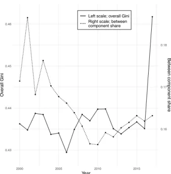
We refer again to the data already presented and we still consider the provincial based aggregation. Thus, the Gini index measures the inequality in the municipal per-class income distribution; and the between and the within component share represent the contributions, respectively, of the inter and intra-provinces diversity to the overall inequality. The values of the share of the proposed between component on the Gini index are plotted in Figure 7 - right scale. The path of the within component share can be easily derived by a reflection and a one unit long vertical translation, because the two components complement to the overall Gini. The Gini index is reported too, but on the left scale. The share of the components seems to be independent from the overall value of the index. Indeed, the latter varies quite irregularly during the considered period, while Sbshows

an initial marked decreasing trend followed by a light recovery; the converse holds for the within component share. As it is evident, we can deliver a lot of information about the inequality and its subgroup distribution by a simple plot.

It is also possible to inform on the contributions which the two components provide to the Gini index percentage variation. The Gini index yearly percentage variations are reported in Figure 8 along with the relative contributions of the change in the between component. Despite, as shown in Figure 7, for this aggregation level the between component has a minority share over the Gini index, its contribution on the Gini index path has been relevant. In the first years of the period under consideration the changes in the between inequality have mainly acted restraining the effects of the variations of the within inequality on the Gini index path. Conversely, the two spatial components have affected the overall inequality in the same direction since 2010. From the results shown for the between component, conclusions on the within inequality can also be easily evinced. This is the main advantage of having a two highly informative components decomposition in empirical contexts.

● ● ● ● ● ● ● ● ● ● ● ● ● ● ● ● ● ● ● ● ● ● ● ● ● ● ● ● ● ● ● ● ● ● ● ● 0.43 0.44 0.45 0.46 0.16 0.17 0.18 2000 2005 2010 2015 Year Ov er all Gini Betw

een component share

Left scale; overall Gini Right scale; between component share

Figure 7: Time series of the share of the proposed between compo-nent over the Gini index - left scale. Gini index trajectory of the municipal per-classes income dis-tribution - right scale.

7 Conclusions

Many spatial concentration measures have been developed in the literature. A recent line of re-search convincingly considers the Gini index as a source from which to derive an effective spatial concentration measure. A certain spatial decomposition of the inequality index has to be em-ployed for this purpose.

The most common spatial Gini index decomposition have been considered in this work. They consist of three components: a residual term augment the sum of the two spatial components, which measure the within and the between group inequality. When the groups do not overlap this term generates some drawbacks w.r.t. our aim of assessing spatial concentration, as we ex-plained in Section 2, and represents a cost in a descriptive context or a regression task in terms of both interpretability and parsimony. Furthermore, the between components of the considered decompositions are designed so that groups with similar means present low levels of territorial inequality regardless of the potential different dispersion within each group. This is an oversim-plification that should be avoided if the distance in the overall group distributions is of interest and the groups overlap.

In order to overcome these two potential drawbacks, in Section 3 and Section 4 we have pre-sented a Gini index decomposition for a population partitioned in groups. It is only composed by the two spatial components. As far as we know this is the first Gini index spatial decomposition proposal for partitioned populations to avoid the residual term. In addition, the between compo-nent relies directly on the individual incomes, hence the overall group income distributions are considered while accounting for territorial inequality.

We have demonstrated that the two components have a correct starting point and move in the right direction and proportion with reference to different scenarios. Indeed, they strongly and positively correlate with two related benchmarks developed to measure the within and the between inequal-ity following an axiomatic approach. In other words, the components approximately provide all the information contained in the benchmarks and observe their axiomatically derived properties, despite the fact they are derived with a decomposition boundary - and not independently as for the benchmarks. Contrariwise, the decomposition boundary strengthens the informativeness of the components. It ensures their collinearity with the Gini index and consequently provides

rele-−2 0 2 4 6 2001 2006 2011 2016 Year P ercentage v ar iation

Overall Gini % variation Between component contribution

Figure 8: Gini index yearly per-centage variation and contribution of the change of the between com-ponent.

vant advantages in a descriptive context or a regression task in terms of both interpretability and parsimony.

The correlation values we refer to were calculated in Section 5 by simulations. Many contexts have been considered by varying the simulation parameters and results appear to be robust. In Section 6 we strengthened the reliability of the simulation algorithm and of the correlation esti-mates by considering the municipality based Income and principal Irpef variables statistical data available on the Open-Source Data released by the Department of Finance of the Italian Ministry of Economy and Finance. In addition, an illustration of the advantages ensured by the proposed decomposition - in terms of informativeness and interpretability in a spatial empirical context - is provided.

References

Allison, Paul D. “Measures of inequality”. In: American sociological review (1978), pp. 865–880. Arbia, Giuseppe. “The role of spatial effects in the empirical analysis of regional concentration”.

In: Journal of Geographical systems 3.3 (2001), pp. 271–281.

Arbia, Giuseppe and Gianfranco Piras. “A new class of spatial concentration measures”. In: Com-putational Statistics & Data Analysis 53.12 (2009), pp. 4471–4481.

Bandourian, Ripsy, James McDonald, and Robert S Turley. “A comparison of parametric models of income distribution across countries and over time”. In: Luxembourg income study working paper (2002).

Bhattacharya, Nath and B Mahalanobis. “Regional disparities in household consumption in In-dia”. In: Journal of the American Statistical Association 62.317 (1967), pp. 143–161. Bickenbach, Frank and Eckhardt Bode. “Disproportionality measures of concentration,

special-ization, and localization”. In: International Regional Science Review 31.4 (2008), pp. 359– 388.

Bourguignon, Francois. “Decomposable income inequality measures”. In: Econometrica: Journal of the Econometric Society (1979), pp. 901–920.

Campante, Filipe R and Quoc-Anh Do. “Inequality, Redistribution, and Population”. In: (2007). Dagum, Camilo. “A new approach to the decomposition of the Gini income inequality ratio”. In:

Empirical Economics (1997), pp. 515–531.

— “Inequality measures between income distributions with applications”. In: Econometrica (pre-1986) 48.7 (1980), p. 1791.

Ebert, Udo. “Measures of distance between income distributions”. In: Journal of Economic The-ory 32.2 (1984), pp. 266–274.

— “The decomposition of inequality reconsidered: Weakly decomposable measures”. In: Math-ematical Social Sciences 60.2 (2010), pp. 94–103.

Ellison, Glenn and Edward L Glaeser. “Geographic concentration in US manufacturing industries: a dartboard approach”. In: Journal of political economy 105.5 (1997), pp. 889–927.

Hyndman, Rob J and Yanan Fan. “Sample quantiles in statistica packages”. In: The American Statistician 50.4 (1996), pp. 361–365.

Kline, Patrick and Enrico Moretti. “People, Places, and Public Policy: Some Simple Welfare Economics of Local Economic Development Programs”. In: Annual Review of Economics 6.1 (2014), pp. 629–662.

Lambert, Peter J and J Richard Aronson. “Inequality decomposition analysis and the Gini coeffi-cient revisited”. In: The Economic Journal 103.420 (1993), pp. 1221–1227.

Mookherjee, Dilip and Anthony Shorrocks. “A decomposition analysis of the trend in UK income inequality”. In: The Economic Journal 92.368 (1982), pp. 886–902.

Moran, Patrick AP. “Notes on continuous stochastic phenomena”. In: Biometrika 37.1/2 (1950), pp. 17–23.

Neumark, David and Helen Simpson. “Place-based policies”. In: Handbook of regional and urban economics. Vol. 5. Elsevier, 2015, pp. 1197–1287.

Ord, J Keith and Arthur Getis. “Local spatial autocorrelation statistics: distributional issues and an application”. In: Geographical analysis 27.4 (1995), pp. 286–306.

Pyatt, Graham. “On the interpretation and disaggregation of Gini coefficients”. In: The Economic Journal 86.342 (1976), pp. 243–255.

Radaelli, Paolo. “On the decomposition by subgroups of the Gini index and Zenga’s uniformity and inequality indexes”. In: International Statistical Review 78.1 (2010), pp. 81–101. Rao, VM. “Two decompositions of concentration ratio”. In: Journal of the Royal Statistical

Soci-ety. Series A (General) 132.3 (1969), pp. 418–425.

Rey, Sergio J and Richard J Smith. “A spatial decomposition of the Gini coefficient”. In: Letters in Spatial and Resource Sciences 6.2 (2013), pp. 55–70.

Rodr´ıguez-Pose, Andr´es. “The revenge of the places that don’t matter (and what to do about it)”. In: Cambridge Journal of Regions, Economy and Society 11.1 (2018), pp. 189–209.

Shorrocks, Anthony F. “Inequality decomposition by population subgroups”. In: Econometrica: Journal of the Econometric Society (1984), pp. 1369–1385.

— “On the distance between income distributions”. In: Econometrica: Journal of the Economet-ric Society (1982), pp. 1337–1339.

— “The class of additively decomposable inequality measures”. In: Econometrica: Journal of the Econometric Society (1980), pp. 613–625.

Shorrocks, Anthony and Guanghua Wan. “Spatial decomposition of inequality”. In: Journal of Economic Geography 5.1 (2005), pp. 59–81.

Yitzhaki, Shlomo. “Economic distance and overlapping of distributions”. In: Journal of Econo-metrics 61.1 (1994), pp. 147–159.

Yitzhaki, Shlomo and Robert I Lerman. “Income stratification and income inequality”. In: Review of income and wealth 37.3 (1991), pp. 313–329.

Appendix

On the approximation due to the quantilisation procedure

The first section of this appendix is due in order to assess the quantilisation procedure, quantify the magnitude of the approximation incurred and identify the optimal definition of quantile and the value of n to be selected.

Recall that, definingw = (w1, . . .wK), we suggested the value n =wn|.

● ● ● ● ● ● ● ● ● ● ● ● 0.0 0.2 0.4 0.6 0.8 1.0 0e+00 2e − 04 4e − 04 6e − 04 8e − 04 Selected probability MSE   Sb rSb    ● 0 0.002 0.004 0.006 0.009 0.013 0.017 0.022 0.027 MAE   Sb rSb   

● _{Left scale; MSE}

Right scale; MAE

(a) MSE (left scale) and MAE (right scale) of the 150

relative differences in Sbfor different choices of n.

0.0 0.2 0.4 0.6 0.8 1.0 − 0.05 0.00 0.05 0.10 Selected probability Sb − Sb e Sb e ● ● ● ● ● ● ● ● ● ● ● ● ● ● ● ● ● ● ● ● ● ● ● ● ● ● ● ● ● ● ● ● ● ● ● ● ● ● ● ● ● ● ● ● ● ● ● ● ● ● ● ● ● ● ● ● ● ● ● ● ● ● ● ● ● ● ● ● ● ● ● ● ● ● ● ● ● ● ● ● ● ● ● ● ● ● ● ● ● ● ● ● ● ● ● ● ● ● ● ● ● ● ● ● ● ● ● ● ● ● ● ● ● ● ● ● ●

(b) Boxplots of the 150 relative differences in Sbfor

different choices of n.

Figure 9: Between component share relative approximation for different choices of n. The ap-proximation is evaluated considering the 150 values of the relative difference in the between share obtained by the quantilisation procedure w.r.t. the one obtainable employing the exact approach. This expression determines n as the average of the nk, each weighted by the related share of

pop-ulation wk. The performance of this value are firstly shown in Figure 9, where approximation is

evaluated looking at the relative discrepancy between the two values of Gb

G obtained employing

the exact or the quantilisation method. More precisely, let Sb=GGb the between component share

obtained by the quantilisation method and Se

b=G

e b

Ge the same share in the exact approach. The

relative discrepancy is measured by the Mean and the Absolute Squared Errors of Sb

Se b w.r.t. 1 = Se b Se b

obtained running 150 simulations - MSE⇣Sb

Se b ⌘ =E⇣Sb Se b 1 ⌘2 and MAE⇣Sb Se b ⌘ =Eh Sb Se b 1 i . In other words in each simulation, for different choices of n, we looked at the relative difference of the between share obtained by the quantilisation procedure w.r.t. the one obtainable employing the exact approach. The results are summarised by averaging the square or the absolute errors. The simulation procedure flows as follow. In each running lognormal-distributed incomes with a vector of sizesn are drawn as described in the second section of this Appendix. The different choices of n are its minimum value, its deciles and the value obtained by eq. (12). The vector n is also drawn and we imposed some constraint on its elements to ensure affordable values for the mcm when employing the exact approach. To be specific, we firstly specified K (= 5, 10 or 20). Then we built a vectormul composed by the divisors of 24₃3_{5 belonging to an interval}