On the RR Lyrae Stars in Globulars. V. The Complete Near-infrared
(JHK
s) Census of ω
Centauri RR Lyrae Variables
*V. F. Braga1,2,3,4 , P. B. Stetson5 , G. Bono3,6 , M. Dall’Ora7 , I. Ferraro6, G. Fiorentino8 , G. Iannicola6, M. Marconi7 , M. Marengo9 , A. J. Monson10, J. Neeley9 , S. E. Persson10, R. L. Beaton10 , R. Buonanno3,11, A. Calamida12 , M. Castellani6, E. Di Carlo11, M. Fabrizio4 , W. L. Freedman13, L. Inno14, B. F. Madore10 , D. Magurno3, E. Marchetti15, S. Marinoni4, P. Marrese4, N. Matsunaga16, D. Minniti1,2,17 , M. Monelli18 , M. Nonino19, A. M. Piersimoni11, A. Pietrinferni11,
P. Prada-Moroni20,21, L. Pulone6, R. Stellingwerf22, E. Tognelli20,21, A. R. Walker23, E. Valenti15 , and M. Zoccali1,24
1
Instituto Milenio de Astrofisica, Santiago, Chile 2
Departamento de Fisica, Facultad de Ciencias Exactas, Universidad Andres Bello, Fernandez Concha 700, Las Condes, Santiago, Chile 3
Department of Physics, Università di Roma Tor Vergata, via della Ricerca Scientifica 1, I-00133 Roma, Italy 4
SSDC, via del Politecnico snc, I-00133 Roma, Italy 5
NRC-Herzberg, Dominion Astrophysical Observatory, 5071 West Saanich Road, Victoria BC V9E 2E7, Canada 6
INAF-Osservatorio Astronomico di Roma, via Frascati 33, I-00040 Monte Porzio Catone, Italy 7
INAF-Osservatorio Astronomico di Capodimonte, Salita Moiariello 16, I-80131 Napoli, Italy 8
INAF-Osservatorio Astronomico di Bologna, Via Ranzani 1, I-40127 Bologna, Italy 9
Department of Physics and Astronomy, Iowa State University, Ames, IA 50011, USA 10
The Observatories of the Carnegie Institution for Science, 813 Santa Barbara St., Pasadena, CA 91101, USA 11
INAF-Osservatorio Astronomico d’Abruzzo, Via Mentore Maggini snc, Loc. Collurania, I-64100 Teramo, Italy 12
National Optical Astronomy Observatory, 950 N Cherry Avenue, Tucson, AZ 85719, USA 13
Department of Astronomy & Astrophysics, University of Chicago, 5640 South Ellis Avenue, Chicago, IL 60637, USA 14
Max Planck Institute for Astronomy Königstuhl 17 D-69117, Heidelberg, Germany 15
European Southern Observatory, Karl-Schwarzschild-Str. 2, D-85748 Garching bei Munchen, Germany 16
Kiso Observatory, Institute of Astronomy, School of Science, The University of Tokyo, 10762-30, Mitake, Kiso-machi, Kiso-gun, 3 Nagano 97-0101, Japan 17
Vatican Observatory, V00120 Vatican City State, Italy 18
Instituto de Astrofísica de Canarias, Calle Via Lactea s/n, E-38205 La Laguna, Tenerife, Spain 19
INAF, Osservatorio Astronoico di Trieste, Via G.B. Tiepolo 11, I-34143 Trieste, Italy 20
INFN, Sezione di Pisa, Largo Pontecorvo 3, I-56127, Pisa, Italy 21
Dipartimento di Fisica“Enrico Fermi,” Università di Pisa, Largo Pontecorvo 3, I-56127, Pisa, Italy 22
Stellingwerf Consulting, 11033 Mathis Mtn Rd SE, Huntsville, AL 35803, USA 23
Cerro Tololo Inter-American Observatory, National Optical Astronomy Observatory, Casilla 603, La Serena, Chile 24
Pontificia Universidad Catolica de Chile, Instituto de Astrofisica, Av. Vicuña Mackenna 4860, Santiago, Chile Received 2017 December 6; revised 2018 February 5; accepted 2018 February 5; published 2018 March 6
Abstract
We present a new complete near-infrared (NIR, JHKs) census of RR Lyrae stars (RRLs) in the globular ω Cen
(NGC 5139). We collected 15,472 JHKsimages with 4–8 m class telescopes over 15 years (2000–2015) covering a
sky area around the cluster center of 60×34 arcmin2. These images provided calibrated photometry for 182 out of the 198 cluster RRL candidates with 10 to 60 measurements per band. We also provide new homogeneous estimates of the photometric amplitude for 180(J), 176 (H) and 174 (Ks) RRLs. These data were supplemented
with single-epoch JKs magnitudes from VHS and with single-epoch H magnitudes from 2MASS. Using
proprietary optical and NIR data together with new optical light curves (ASAS-SN) we also updated pulsation periods for 59 candidate RRLs. As a whole, we provide JHKsmagnitudes for 90 RRab(fundamentals), 103 RRc
(first overtones) and one RRd (mixed-mode pulsator). We found that NIR/optical photometric amplitude ratios increase when moving fromfirst overtone to fundamental and to long-period (P>0.7 days) fundamental RRLs. Using predicted period–luminosity–metallicity relations, we derive a true distance modulus of 13.674± 0.008±0.038 mag (statistical error and standard deviation of the median) based on spectroscopic iron abundances, and of 13.698±0.004±0.048 mag based on photometric iron abundances. We also found evidence of possible systematics at the 5%–10% level in the zero-point of the period–luminosity relations based on the five calibrating RRLs whose parallaxes had been determined with the HST.
Key words: globular Clusters: individual(ω Centauri) – stars: distances – stars: horizontal-branch – stars: variables: RR Lyrae
Supporting material: machine-readable table
1. Introduction
There is mounting evidence that deep and accurate near-infrared (NIR) photometry presents several indisputable advantages over optical photometry concerning distance determinations. The obvious advantage is the lower sensitivity to reddening(i.e., uncertainties in the reddening values or the presence of differential reddening), but the advantages become
The Astronomical Journal, 155:137 (27pp), 2018 March https://doi.org/10.3847/1538-3881/aaadab
© 2018. The American Astronomical Society. All rights reserved.
* This publication makes use of data gathered with the Magellan/Baade Telescope at Las Campanas Observatory, the Blanco Telescope at Cerro Tololo Inter-American Observatory, NTT at La Silla(ESO Program IDs: 64.N-0038 (A), 66.D-0557(A), 68.D-0545(A), 073.D-0313(A), ID 073.D-0313(A) and 59. A-9004(D)), VISTA at Paranal (ESO Program ID: 179.A-2010) and VLT at Paranal(ESO Program ID: ID96406).
even more relevant when dealing with primary distance indicators such as Cepheids (classical and type-II) and RR Lyrae (RRL) stars. Theory and observations indicate that the dispersions of period–luminosity (PL) relations steadily decrease when moving from optical to NIR bands. The PL relations can be derived neglecting the color term, i.e., the width in temperature of the instability strip, and this assumption becomes less severe in the NIR regime.
Here, we will focus on the RRLs. In the optical(BV ) bands they typically obey a magnitude versus metallicity relation, and the PL relation becomes evident only for wavelengths longer than the R band (Marconi et al.2015; Braga et al. 2016). The
slope of the PL relation steadily increases from the R- to the J-band and attains an almost constant value for wavelengths longer than 2.2μm (Madore et al. 2013; Beaton et al. 2016; Neeley et al. 2017). The amplitudes display a similar trend:
they attain their largest values in the U band and approach an almost constant value for wavelengths longer than 2.2μm (Braga et al.2015; Neeley et al.2015; M. Marconi et al. 2018, in preparation). This empirical evidence and theoretical considerations both indicate that luminosity variation in the optical regime is mainly dominated by effective temperature variation, while in the NIR regime it is mainly dominated by radius variation(Madore et al.2013; Bono et al.2016).
The metallicity dependence of RRLs, in contrast with classical Cepheids, is quite well established. Theory and observations indicate that an increase in metal content makes RRLs fainter. The above evidence makes RRLs key standard candles, and they provide a very promising opportunity to provide an independent calibration of secondary distance indicators and to constrain possible systematics between low-mass/old and intermediate-mass/young distance indicators (Beaton et al. 2016). However, we still lack firm empirical
estimates of the zero-point, the slope, and the metallicity dependence of the diagnostics adopted to estimate individual RRL distances.
In this context, cluster RRLs play a crucial role, since we have detailed knowledge of both the age and the chemical composition of their progenitors. In particular, the RRLs in ω Cen appear to be an ideal laboratory, even though we are still lacking solid constraints on the formation and evolution of this peculiar globular. The reasons are as follows.
(a) ω Cen includes almost 200 RRLs and they are almost equally split between fundamental andfirst overtone pulsators. This suggests that the instability strip is well populated both in the red/cool and in the blue/hot region.
(b) Current empirical evidence indicates that RRLs in ω Cen cover a metallicity range of at least one dex. This makesω Cen a fundamental testbed to constrain the metallicity dependence, since the depth effects are negligible compared with its distance.
(c) ω Cen hosts at least eight alternative distance indicators: (1) tip of the red giant branch (Bellazzini et al. 2004; Bono et al.2008); (2) HB luminosity level (VandenBerg et al.2013);
(3) Type II Cepheids (Matsunaga et al. 2006; Navarrete et al.2017); (4) Miras (Feast1965); (5) SX Phoenicis variables
(McNamara 2000); (6) eclipsing binaries (Thompson
et al. 2001); (7) the white dwarf cooling sequence (Ortolani
& Rosino 1987; Calamida et al. 2008); (8) an astrometric
distance (van de Ven et al. 2006). This provides a unique
opportunity to constrain the systematics affecting standard candles that originate from different physical mechanisms.
In spite of the quoted indisputable advantages, the NIR investigations lag when compared with optical ones. Accurate NIR time series data for a significant fraction of ω Cen RRLs were provided for thefirst time by Del Principe et al. (2006).
They adopted NIR time series data collected with SOFI at NTT and provided homogeneous mean JKs magnitudes for 180
variables(114 based on proprietary data: 81 J, 119 Ksimages).
More recently, Navarrete et al.(2015,2017) collected NIR
time series data(252 J and 600 Ksimages) of ω Cen with the
VIRCAM at ESO VISTA telescope. They discovered four new candidate RRLs(two cluster members and two nonmembers). They also provided new mean JKsmagnitudes for 187 out of
the 198 RRLs. Using NIR PL relations for both RRLs and Type II Cepheids they found a weighted-average true distance modulus toω Cen of 13.708±0.035 mag.
However, our data sets provide a few key advantages with respect to the quoted literature works:(1) full coverage of light curves in the H band;(2) the possibility to complement our data with proprietary optical data; (3) a better pixel scale that provides a more accurate photometric reduction of blended sources in the central region of the cluster.
Although the cluster and field RRLs have been at the crossroads of an empirical effort of paramount importance (OGLE, CATALINA, Pan-STARRS, VVV) we still lack a detailed analysis of the pulsation properties (photometric amplitudes, topology of the instability strip) of RRL stars in the NIR regime. We are interested in providing a complete NIR census of RRLs in ω Cen as a stepping stone for future developments.
(i) To derive new and accurate NIR (JHKs) template light
curves. Future ground-based extremely large telescopes and space telescopes(JWST, EUCLID, WFIRST) will allow us to measure RRLs in Local Volume galaxies. It is plausible to assume that they will allow us to collect only a few random points, so NIR templates are essential to improve the accuracy of the mean magnitudes.
(ii) By taking advantage of the coupling between optical and NIR mean magnitudes, to provide a simultaneous estimate of distance, reddening, and metal content adopting an approach similar to that used by Inno et al.(2016) for classical Cepheids
in the Large Magellanic Cloud(LMC).
To accomplish these goals we took advantage of specific NIR(JHKs) time series data collected with SOFI at NTT, with
NEWFIRM at CTIO and with FourStar(Persson et al.2013) at
Magellan.
The structure of the paper is as follows. In Section 2 we present the NIR JHKsphotometric data sets. In this section we
introduce not only the NIR time series, but also show the cluster area covered by different data sets and their NIR color– magnitude diagrams (CMDs). The entire sample of cluster RRLs is presented in Section3. Sections3.3and3.2deal with the the phasing of the data (light curves) and with period estimates, while in Section3.3we discuss the analyticalfits to the light curves and the estimates of both mean magnitudes and photometric amplitudes. The comparison with mean magni-tudes available in the literature is discussed in Section 3.4. Section4.1introduces the topology of the instability strip both in NIR and in NIR–optical CMDs, while in Section 4.2 we outline the properties of the variables in the luminosity amplitude versus logarithmic period(Bailey diagram) together with optical–NIR and NIR photometric amplitude ratios. In Section 5 we present NIR PL relations and discuss in detail 2
their dependence on the metal content. The new distance determinations to ω Cen, based on NIR PL relations, and the comparison with literature estimates are discussed in Section6. The summary of the mainfindings of the current investigation and the future developments of the overall project are outlined in Section7.
2. NIR Photometric Data Sets
A complete synopsis of our NIR data sets is given in Table1. The grand total of our images is 15,472: 5102 in J, 4872 in H and 5498 in Ks, collected over 15 years (2000 January–2015
January).
The majority (∼95%) of our data were collected with the FourStar imager (pixel scale: 0.16 arcsec/pix) at the 6.5 m Magellan-Baade telescope at Las Campanas duringfive nights in 2013 June (10,800 images, Figure 1) and three nights in
2015 January (3979 images, Figure 2; one exposure was missing the data from chip 3). The seeing during the 2013 run was better than 1 290% of the time and better than 0 85 half of the time. Frames from the run of 2015 were collected in excellent seeing conditions: 90% of the time it was better than 0 6 and, half of the time it was better than 0 45. The fifteen pointings of the 2013 and 2015 data are almost the same, and cover a sky area of 60×34 arcmin2 (∼0.57 degree2). The dithering pattern is made up byfive single exposures.
Around 5% of our images were collected with the NEW-FIRM instrument(0.4 arcsec/pix) at the CTIO 4.0 m telescope during one night in 2010 May(308 images) and with the SOFI camera (0.25 arcsec/pix) at the NTT 3.6 m telescope at La Silla(314 images) during 2000–2005. Only a few of these data (12 SOFI images) were collected in the H band. These data cover∼1480 arcmin2(one NEWFIRM pointing and five SOFI pointings, Figure 3) and are completely contained within the
FourStar area. For 90% of the time, the seeing was better than 1 0, and half of the time better than 0 7. We point out that the images used by Del Principe et al.(2006) for their photometry
are a subsample(200 images) of our SOFI data set.
Finally, we also collected 70 images with MAD at VLT 8.0 m, during 2007 April 3–5 and 2007 June 1 and 3. These data were collected with a seeing of 0 7–0 9 but the AO unit of the instrument provided a mean FWHM smaller than 0 2 for 90% of the images and smaller than 0 1 for half of the images. The two pointings covered a sky area of 2 arcmin2 (see Figure4).
As a whole, the entire NIR data set for ω Cen exceeds the capabilities of our computers for simultaneous reduction, so we performed DAOMASTER and ALLFRAME on four
independent subsamples: (1) the 2013 June Las Campanas data, hereinafter LCO13;(2) the 2015 January Las Campanas data, hereinafter LCO15;(3) the other natural-seeing observa-tions, hereinafter “other”; (4) AO assisted data, hereinafter MAD. After the completion of the profile-fitting photometry the four catalogs were merged to assign a common numbering scheme to the individual stars.
The photometry was calibrated on the basis of 2MASS stars contained within our images. We considered only 2MASS All-Sky Point Source Catalog photometric measurements that had been assigned photometric quality class“A.” This quality class corresponds to magnitude determinations in the J, H, or Ks Table 1
Log of the Observations ofω Cen in NIR Bands
Run ID Dates Telescope Camera J H Ks other multiplex
1 giuseppe 2000 Jan 13–2004 Jun 04 ESO NTT 3.6 m SOFI 109 L 130 L K
2 milena 2004 Jun 03 ESO NTT 3.6 m SOFI 15 L K L K
3 anna 2005 Apr 02 ESO NTT 3.6 m SOFI 12 12 36 L K
4 calamid 2007 Apr 03–Jun 03 ESO VLT 8.0 m MAD 6 L 9 55 K
5 blanco 2010 May 24–25 CTIO 4.0 m Newfirm 25 L 52 L 4
6 lco1306 2013 Jun 25–29 Magellan6.5 m FourStar 900 900 900 L 4
7 lco1501 2015 Jan 26–27 Magellan6.5 m FourStar 315 315 365 L 4
Notes. 1 ESO program IDs 64.N-0038(A), 66.D-0557(A), 68.D-0545(A), 073.D-0313(A); observer(s) unknown; 2 ESO program ID 073.D-0313(A); observer unknown; 3 ESO program ID 59.A-9004(D); observer unknown; 4 ESO program ID “ID96406”; observer unknown; “other”=Brackett γ; 5 Proposal ID “noao”; observers Allen, DePropris; 6 Observer A. Monson; 7 Observer N. Morrel.
Figure 1.Distribution on the sky(arcseconds) of the photometry performed on NIR(JHKs) images collected with FourStar at Magellan in 2013 (LCO13). This data set covers a cluster area of 60×34 arcmin2. The color coding is correlated with the number of measurements(see the right bar). A black plus marks the position of the cluster center(Braga et al.2016). The black circle
marks the half-mass radius(300 arcsec; Harris1996).
Figure 2.Same as in Figure 1, but for NIR(JHKs) images collected with FourStar at Magellan in 2015(LCO15). This data set covers a cluster area of 60×34 arcmin2.
3
bandpass with a signal-to-noise ratio 10 (σ(magnitude) estimated to be 0.109 mag). Matches between the 2MASS stars and entries in our joint catalog were determined by astrometric agreement within a tolerance of 1arcsec; matches satisfying this criterion agreed positionally with a standard deviation of 0.15 arcsec in the x (∼right ascension) direction and 0.14 arcsec in y(∼declination). The 2MASS magnitudes were used as standard measurements to calibrate our instru-mental magnitudes using transformation equations employing linear color terms. Individual stars displaying large residuals from preliminary fits were gradually discarded until the transformation relied only on 12,802 individual 2MASS stars with fitting residuals <0.20 mag in at least one of the three bandpasses.
Our natural-seeing observations ofω Cen were calibrated to the 2MASS photometric system on the basis of these transformation equations. An additional 172 fainter but well-isolated stars that were well-observed in our data sets were selected to serve as secondary calibrators for the MAD observations.
In reducing the NIR data set forω Cen we adopted a double strategy. We performed ALLSTAR/ALLFRAME photometry over the entire set of NIR images. This approach is required to have accurate time series data to estimate the pulsation parameters. Moreover, we also performed an independent photometric reduction based upon the stacked images. This approach was adopted to improve the detection of faint stars and to provide a very accurate and deep NIR(JHKs) catalog, with no attempt at
time resolution.
We have derived accurate CMDs from the current photo-metry, covering both the bright region typical of red giant branch (RGB) and asymptotic giant branch stars (up to Ks∼8.5 mag thanks to the SOFI data), but also ∼1.5–2.5
magnitudes fainter than the main sequence turn-off region (FourStar data, see Figure 5). The mean squared sums of the
J- and Ks-band photometric errors in different magnitude bins
are plotted as red error bars on the right of each panel. The stars plotted in the above CMDs have been selected by the χ parameter, which quantifies the deviation between the star profile and the adopted point-spread function (PSF), and the sharpness ( sha∣ ∣<0.7), which indicates the difference in broadness of the individual stars compared with the PSF and is used to reject non-stellar sources. In passing we note that PSF photometry of individual images is essential to improve the precision of individual measurements of variable stars. The identification and fitting of faint sources located near the variable stars provides an optimal subtraction of light contamination from neighboring stars.
The effect of seeing is clear when we compare the CMDs in panels(a) and (b): the telescope and the camera are the same, but the better seeing during 2015 allowed us to gain∼0.3 mag in depth. However, the better seeing also caused a larger spread in color of stars on the upper RGB (Ks<12 mag), due to a
fainter level of saturation.
The effect of the seeing and of the pixel scale of the instrument is also clear when comparing the LCO13, LCO15 and other data sets. LCO15 is, in fact, ∼0.3 mag deeper than the other two and that with the least populated RGB and the sharpest blue and extreme horizontal branch. On the other hand, the other data set has a better populated upper RGB.
Finally, the MAD data set is the deepest, but most importantly, shows the least amount of contamination by field stars—which is quite clear in the two LCO data sets at J–Ks∼0.85 mag—since the observed sky area is small and very
close to the cluster center. These are clear advantages of using AO corrections for the CMD observations (but an obvious disadvantage for acquiring a large sample of RR Lyraes).
3. RR Lyrae Stars
We adopt Table 2 in Braga et al.(2016) as our reference list
of RRL candidates inω Cen, but exclude NV433 as suggested by Navarrete et al. (2015). Note that we use the term “RRL
candidates” because we lack solid, homogeneous constraints on their membership, other than considerations on their distance from the cluster center, mean magnitude, and proper motions for a few of them(van Leeuwen et al.2000; Bellini et al.2009).
Therefore, we kept 198 out of 199 objects from the quoted list. According to the literature, eight of these 198 stars are confirmed nonmembers (V84, V168, V175, V181, V183, V283, NV457, NV458, van Leeuwen et al. 2000; Fernández-Trincado et al.2015; Navarrete et al.2015). The classification
of V68 and V84 is ambiguous because, until now, their periods
Figure 3. Same as in Figure1, but for NIR (JHKs) images collected with different telescopes(“other” data set, see text for more details). This data set covers a cluster area of 27×33 arcmin2.
Figure 4.Same as in Figure1, but for NIR(JKs) images collected with the MCAO system (MAD) that was available at VLT. The individual pointings cover an area of 1×1 arcmin2.
4
and their positions in both the CMD and in the period– magnitude plane did not allow a clear discrimination between RRL and anomalous Cepheid (AC) classifications. For three stars (V171, V178 and V179) neither periods nor mean magnitudes were available, while for V182, only the period was known. However, for thefirst time since these four stars were classified as variables (Wilkens 1965; Sawyer Hogg
1973), we have retrieved multi-epoch photometry for them.
Thus, we have data for all the RRL candidates ofω Cen. For the master catalog for the ALLFRAME runs on our NIR data, we adopted the catalog generated during the photometric reduction of the optical (UBVRI) data (see Section 2 of Braga et al.2016). This allowed us to assign to the NIR point sources
the same identification numbers as the optical sources, providing an unambiguous identification of all the stars within the sky area covered by our images and an accurate cross-match of the optical and NIR catalogs. The cross-cross-match allowed us to retrieve the UBVRI light curves of NV411, that we had missed in Braga et al. (2016).
3.1. Light Curves
The median number of phase points in the light curves obtained from our NIR data is 109, 77, and 136 for the J, H, and Ks bands, respectively. The median of the photometric
errors on the single-epoch magnitudes are 0.012, 0.013, and 0.018 mag(J, H, and Ks). However, there is a large difference
in the photometric errors between the FourStar data (median 0.015 mag in the JHKs bands) and the data sets blanco and
milena (subsets of the other data set, Table 1, median 0.025 mag in all bands); moreover, errors on the single phase points can be as large as 0.2 mag.
As a preliminary step before analyzing the light curves, we binned the phase points to combine data from the same dithering sequence. The time step was ∼90 s for the LCO dithering sequence and ∼900 s for the other data. We tested different binning methods, including simple intensity mean, median, and weighted intensity mean. We adopted the weighted intensity mean because it provides smoother light curves. Note that, before averaging the single phase points, we performed a sigma clipping at a 3σ level to reject the outliers.
The rejected phase points were probably obtained from images with either a lower quality or for which the photometric solution was not optimal. The fraction of phase points that was rejected in this step was smaller than 5%.
Note that the binning of the data was applied to the dithering sequences of individual data sets. The duration of a dithering sequence is a tiny fraction of the pulsation period of an RRL. Moreover, the bulk of the NIR data were collected as time series data, therefore, possible changes in the pulsation period minimally affect the binning of the data. After the binning process, we ended up with light curves including a median number of phase points of 25(J), 17 (H) and 30 (Ks), respectively.
3.2. Pulsation Periods
We have already mentioned in Section2that the majority of our NIR data were collected in 2013 and 2015. On the other hand, most of the optical time-series data were collected between 1995 and 1999. The remarkable overall time coverage(27 years) of optical plus NIR data allowed us to revise the period estimates derived in Braga et al.(2016). We have derived the new period
estimates by adopting the same method as the quoted paper, based on the Lomb–Scargle periodogram (Scargle 1982). This
method simultaneously folds the time series of all the photometric bands that are available. A visual inspection of the folded light curves and a quantitative estimate of the χ2 allow us to estimate the period. On the basis of our overall optical and NIR photometry, we provide new period estimates for 59 variables. For 17 of them, the new period estimate should be considered as an improvement of the estimate based only on the optical data. For 30 variables, the new estimate suggests an intrinsic period change occurred during the time that passed between the acquisition of the bulk of the optical and NIR data (as indicated in Table 2). For the remaining 12 variables, the
period available in the literature was updated. Note that V171 and V179 had no period at all in the literature.
We point out that our ability to detect period variations for some variables is a consequence of the accuracy of our method to estimate periods. A full analysis of period variations is not within the scope of this paper, so we discuss only a few variables. An extensive analysis of the rate of period change(β)
Figure 5.NIR(Ksvs. J–Ks) color–magnitude diagrams of ω Cen. Error bars display intrinsic errors both in magnitude and in color. To make them visible, they are magnified by a factor of five.
5
Table 2
NIR–JHKs–Mean Magnitudes and Amplitudes for ω Cen RRLs
ID Period(new) Period(old)a Variable fitJb J AJ fitHb H AH fitK
sb Ks AKs
days days type mag mag mag mag mag mag
V3 0.84126158 L RRab P 13.182±0.007 0.353±0.029 P 12.895±0.007 0.300±0.029 S 12.864±0.009 0.285±0.027 V4 0.62731846 L RRab S 13.378±0.008 0.494±0.054 S 13.106±0.008 0.333±0.031 S 13.077±0.009 0.316±0.020 V5c 0.51528002 L RRab S 13.668±0.012 0.441±0.028 S 13.488±0.019 0.354±0.043 S 13.409±0.012 0.334±0.016 V7 0.71303420 L RRab S 13.289±0.005 0.428±0.041 P 13.018±0.006 0.305±0.025 S 12.976±0.006 0.312±0.028 V8 0.52132593 L RRab S 13.577±0.004 0.449±0.056 S 13.341±0.009 0.344±0.018 S 13.305±0.005 0.295±0.017 V9c 0.52335114d 0.52346446 RRab S 13.641±0.010 0.320±0.050 P 13.430±0.005 0.175±0.033 S 13.378±0.009 0.225±0.025 V10 0.37475609e 0.37488161 RRc P 13.551±0.006 0.153±0.013 S 13.316±0.017 L S 13.313±0.009 0.080±0.010 V11c 0.56480650 L RRab S 13.474±0.005 0.248±0.023 S 13.209±0.008 0.189±0.023 S 13.189±0.006 0.196±0.016 V12 0.38677657d 0.38676730 RRc S 13.545±0.011 L S 13.299±0.015 L S 13.281±0.010 K V13 0.66904841 L RRab S 13.315±0.008 0.405±0.026 S 13.039±0.008 0.330±0.028 S 13.011±0.008 0.307±0.015 V14 0.37710263e 0.37712562 RRc S 13.575±0.003 0.205±0.018 S 13.352±0.005 0.113±0.011 P 13.347±0.005 0.110±0.009 V15 0.81065426 L RRab S 13.178±0.006 0.353±0.024 S 12.843±0.008 0.309±0.033 S 12.850±0.007 0.287±0.037 V16 0.33019610 L RRc P 13.688±0.003 0.182±0.015 P 13.468±0.005 0.072±0.009 S 13.481±0.004 0.103±0.010 V18 0.62168636 L RRab P 13.421±0.007 0.525±0.021 S 13.137±0.008 0.246±0.014 S 13.127±0.007 0.323±0.017 V19 0.29955165 L RRc P 13.864±0.004 0.169±0.017 P 13.661±0.004 0.088±0.010 S 13.653±0.005 0.111±0.009 V20 0.61558779e 0.61556372 RRab S 13.438±0.014 0.426±0.038 S 13.114±0.007 0.261±0.021 S 13.100±0.007 0.311±0.019 V21 0.38080948 L RRc S 13.553±0.009 0.198±0.023 S 13.369±0.008 0.118±0.013 S 13.370±0.009 0.110±0.015 V22c 0.39616527d 0.39608414 RRc S 13.536±0.005 0.174±0.014 S 13.292±0.008 0.120±0.012 S 13.289±0.006 0.115±0.012 V23 0.51087033 L RRab S 13.717±0.005 0.441±0.054 P 13.445±0.010 L S 13.396±0.008 0.357±0.029 V24 0.46222155 L RRc P 13.396±0.005 0.162±0.015 S 13.125±0.008 0.120±0.013 S 13.123±0.006 0.093±0.013 V25 0.58851546e 0.58835430 RRab S 13.458±0.009 0.437±0.054 S 13.194±0.008 0.364±0.045 S 13.157±0.012 0.293±0.029 V26 0.78472145 L RRab S 13.222±0.005 0.317±0.027 P 12.927±0.007 0.276±0.024 S 12.875±0.006 0.230±0.020 V27 0.61569276 L RRab S 13.528±0.003 0.237±0.021 P 13.220±0.008 0.210±0.027 S 13.198±0.006 0.248±0.020 V30c 0.40397132e 0.40423516 RRc P 13.521±0.006 0.151±0.009 S 13.263±0.009 0.073±0.011 S 13.246±0.008 0.105±0.013 V32c 0.62036776 L RRab S 13.463±0.004 0.388±0.030 S 13.167±0.006 0.321±0.027 S 13.119±0.006 0.322±0.019 V33 0.60233332 L RRab S 13.409±0.005 0.468±0.045 S 13.146±0.010 0.315±0.026 S 13.141±0.006 0.288±0.021 V34 0.73395501 L RRab S 13.256±0.007 0.325±0.029 S 12.967±0.005 0.248±0.020 S 12.931±0.007 0.281±0.019 V35 0.38683322 L RRc S 13.530±0.007 0.175±0.013 P 13.283±0.008 0.134±0.015 P 13.290±0.008 0.097±0.012 V36 0.37990927e 0.37981328 RRc P 13.529±0.004 0.188±0.015 S 13.305±0.008 0.113±0.011 S 13.295±0.004 0.112±0.015 V38c 0.77905902 L RRab S 13.219±0.003 L S 12.916±0.006 0.185±0.014 S 12.886±0.005 0.214±0.015 V39 0.39338605 L RRc P 13.570±0.005 0.179±0.015 P 13.328±0.007 0.112±0.011 S 13.320±0.007 0.117±0.010 V40 0.63409776 L RRab S 13.407±0.006 0.489±0.061 S 13.129±0.008 0.313±0.031 S 13.095±0.009 0.319±0.029 V41 0.66293383 L RRab S 13.374±0.007 0.381±0.027 S 13.082±0.007 0.339±0.028 P 13.043±0.009 0.328±0.019 V44 0.56753783d 0.56753608 RRab S 13.610±0.005 0.456±0.044 S 13.326±0.006 0.306±0.030 S 13.304±0.007 0.300±0.020 V45c 0.58913452 L RRab S 13.427±0.005 0.545±0.082 S 13.178±0.003 0.323±0.040 S 13.161±0.005 0.336±0.024 V46 0.68696236 L RRab P 13.325±0.003 0.415±0.045 S 13.040±0.003 0.288±0.021 P 13.016±0.005 0.274±0.016 V47 0.48532643d 0.48529500 RRc P 13.320±0.004 0.157±0.016 S 13.077±0.010 0.097±0.016 P 13.067±0.007 0.101±0.013 V49 0.60464946d 0.60464471 RRab S 13.474±0.003 0.422±0.040 S 13.197±0.005 0.273±0.027 P 13.163±0.005 0.282±0.016 V50 0.38616585 L RRc S 13.591±0.004 0.186±0.020 S 13.343±0.007 0.123±0.014 P 13.343±0.005 0.091±0.011 V51 0.57414241 L RRab S 13.466±0.006 0.414±0.040 P 13.179±0.009 0.312±0.021 S 13.161±0.008 0.326±0.020 V52 0.66038704 L RRab S 13.298±0.016 0.468±0.039 S 13.060±0.011 L S 12.977±0.012 0.262±0.022 V54 0.77290930 L RRab P 13.232±0.004 0.308±0.033 S 12.917±0.005 0.281±0.035 P 12.884±0.004 0.253±0.032 V55 0.58166391e 0.58192068 RRab S 13.614±0.004 0.410±0.036 P 13.283±0.108 L S 13.291±0.005 0.250±0.015 V56c 0.56803579 L RRab S 13.642±0.008 0.425±0.039 S 13.346±0.008 0.280±0.021 S 13.343±0.006 0.263±0.018 V57 0.79442230 L RRab S 13.213±0.003 0.269±0.018 S 12.887±0.005 0.204±0.020 S 12.874±0.004 0.230±0.015 V58 0.37985623e 0.36992250 RRc S 13.581±0.007 L P 13.385±0.011 L P 13.370±0.008 K V59c 0.51855138 L RRab S 13.624±0.017 0.385±0.066 P 13.397±0.013 0.312±0.055 T 13.39±0.01 K 6 The Astronomical Journal, 155:137 (27pp ), 2018 March Braga et al.
Table 2 (Continued)
ID Period(new) Period(old)a Variable fitJb J AJ fitHb H AH fitKs
b
Ks AKs
days days type mag mag mag mag mag mag
V62 0.61979638 L RRab S 13.398±0.008 0.457±0.058 S 13.134±0.006 0.369±0.040 S 13.078±0.007 0.288±0.024 V63 0.82595979 L RRab S 13.190±0.003 0.228±0.022 S 12.876±0.004 0.210±0.021 S 12.849±0.004 0.199±0.020 V64 0.34444598d 0.34447428 RRc S 13.634±0.005 0.195±0.018 S 13.409±0.005 0.133±0.013 P 13.413±0.006 0.106±0.012 V66 0.40723082d 0.40727290 RRc S 13.481±0.006 0.163±0.015 S 13.239±0.006 0.113±0.014 S 13.230±0.006 0.097±0.009 V67c 0.56444856 L RRab S 13.593±0.004 0.506±0.048 S 13.323±0.006 0.326±0.029 S 13.310±0.005 0.298±0.019 V68 0.53462524e 0.53476174 RRc/ACep S 13.211±0.006 0.124±0.012 P 12.958±0.007 0.053±0.011 S 12.942±0.005 0.062±0.007 V69c 0.65322088 L RRab S 13.399±0.004 0.376±0.033 S 13.114±0.006 0.273±0.022 S 13.099±0.004 0.272±0.023 V70 0.39081066e 0.39059068 RRc S 13.517±0.005 0.179±0.028 P 13.275±0.006 0.125±0.017 S 13.268±0.005 0.102±0.011 V71 0.35769621d 0.35764894 RRc S 13.624±0.019 L P 13.410±0.010 L S 13.385±0.012 K V72 0.38450448 L RRc S 13.545±0.004 0.181±0.013 P 13.303±0.008 0.130±0.019 S 13.318±0.005 0.102±0.010 V73c 0.57520367 L RRab S 13.489±0.004 0.449±0.048 P 13.236±0.007 0.309±0.027 P 13.210±0.009 0.271±0.025 V74c 0.50321425 L RRab S 13.604±0.005 0.544±0.048 S 13.379±0.014 0.313±0.035 S 13.354±0.007 0.338±0.038 V75 0.42220668e 0.42214238 RRc P 13.424±0.004 0.169±0.015 P 13.159±0.006 0.128±0.015 S 13.164±0.004 0.119±0.010 V76 0.33796008 L RRc P 13.636±0.007 0.171±0.020 P 13.422±0.009 L T 13.47±0.01 K V77 0.42598243e 0.42604092 RRc S 13.448±0.003 0.171±0.022 S 13.190±0.006 0.099±0.012 S 13.184±0.006 0.099±0.012 V79 0.60828692 L RRab S 13.461±0.004 0.469±0.041 S 13.205±0.011 0.325±0.026 S 13.152±0.007 0.306±0.021 V80 0.37719716e 0.37721794 RRc S 13.633±0.005 0.143±0.016 P 13.452±0.009 0.086±0.015 S 13.440±0.009 0.083±0.018 V81 0.38938509 L RRc S 13.535±0.004 0.177±0.013 S 13.300±0.008 0.099±0.014 S 13.285±0.006 0.110±0.009 V82c 0.33576546 L RRc P 13.591±0.004 0.165±0.015 S 13.381±0.005 0.106±0.012 P 13.386±0.007 0.092±0.013 V83 0.35661021 L RRc P 13.602±0.004 0.184±0.018 S 13.377±0.006 0.125±0.016 P 13.377±0.005 0.106±0.015 V84 0.57991785 L RRab/ACep S 13.095±0.006 0.303±0.027 S 12.804±0.008 0.232±0.021 S 12.781±0.009 0.226±0.022 V85 0.74274920 L RRab S 13.314±0.005 0.304±0.025 S 12.997±0.009 0.290±0.022 P 12.957±0.007 0.228±0.019 V86 0.64784141 L RRab S 13.379±0.006 0.430±0.053 S 13.075±0.006 0.386±0.048 P 13.051±0.008 0.290±0.024 V87 0.39594092 L RRc S 13.523±0.007 0.149±0.018 S 13.282±0.012 0.081±0.017 S 13.249±0.011 0.087±0.015 V88 0.69021146 L RRab P 13.373±0.014 0.450±0.044 S 13.119±0.026 0.289±0.041 P 13.049±0.018 0.258±0.036 V89 0.37403725e 0.37417885 RRc S 13.576±0.008 0.177±0.017 P 13.316±0.008 0.116±0.014 S 13.276±0.012 0.123±0.019 V90 0.60340531 L RRab S 13.420±0.016 0.545±0.069 P 13.194±0.012 0.370±0.030 P 13.102±0.010 0.274±0.017 V91 0.89522178 L RRab P 13.086±0.013 0.316±0.019 S 12.754±0.010 0.238±0.019 S 12.722±0.010 0.257±0.018 V94c 0.25393406 L RRc S 13.987±0.009 0.106±0.014 S 13.808±0.009 0.076±0.015 P 13.830±0.008 0.053±0.009 V95 0.40496622 L RRc P 13.501±0.002 0.198±0.016 S 13.250±0.004 0.122±0.014 S 13.258±0.004 0.118±0.013 V96 0.62452166d 0.62452829 RRab S 13.354±0.014 0.365±0.028 S 13.094±0.008 0.241±0.023 S 13.033±0.008 0.309±0.023 V97c 0.69188985 L RRab S 13.321±0.005 0.417±0.026 S 13.022±0.009 0.308±0.021 S 12.995±0.008 0.280±0.016 V98 0.28056563 L RRc S 13.916±0.008 0.196±0.021 S 13.716±0.012 0.120±0.021 S 13.725±0.011 0.094±0.011 V99 0.76617945 L RRab S 13.172±0.009 0.454±0.035 S 12.892±0.014 0.332±0.081 S 12.854±0.009 0.247±0.018 V100 0.55274773 L RRab S 13.631±0.006 0.502±0.062 S 13.341±0.013 0.294±0.027 S 13.329±0.008 0.299±0.021 V101 0.34099950e 0.34094664 RRc S 13.655±0.006 0.120±0.017 S 13.434±0.006 0.038±0.008 S 13.443±0.006 0.046±0.011 V102 0.69139606 L RRab S 13.329±0.004 0.453±0.044 S 13.030±0.006 L S 12.993±0.006 0.290±0.017 V103 0.32885556 L RRc S 13.643±0.008 L S 13.441±0.007 0.078±0.010 S 13.426±0.007 K V104 0.86752592e 0.86656711 RRab S 13.217±0.011 0.174±0.015 S 12.884±0.010 0.199±0.017 P 12.856±0.011 0.168±0.014 V105 0.33533089 L RRc P 13.756±0.003 0.168±0.016 S 13.530±0.004 0.122±0.011 S 13.534±0.004 0.107±0.010 V106c 0.56990293 L RRab P 13.465±0.011 0.513±0.048 P 13.230±0.020 0.301±0.052 T 13.17±0.01 K V107 0.51410378 L RRab S 13.658±0.008 0.446±0.033 S 13.407±0.006 0.376±0.025 S 13.373±0.006 0.313±0.016 V108 0.59445663 L RRab S 13.431±0.008 0.482±0.052 P 13.163±0.011 0.258±0.029 S 13.117±0.011 0.266±0.024 V109 0.74409920 L RRab S 13.259±0.010 0.423±0.038 S 12.964±0.011 L P 12.919±0.009 K V110 0.33210241 L RRc S 13.694±0.008 0.164±0.017 S 13.510±0.009 0.086±0.016 S 13.478±0.009 0.086±0.014 V111 0.76290111 L RRab S 13.234±0.012 0.359±0.030 S 12.984±0.014 0.300±0.028 P 12.861±0.010 0.217±0.018 V112c 0.47435597 L RRab S 13.760±0.016 0.623±0.079 S 13.460±0.013 0.404±0.040 P 13.482±0.016 0.296±0.018 7 The Astronomical Journal, 155:137 (27pp ), 2018 March Braga et al.
Table 2 (Continued)
ID Period(new) Period(old)a Variable fitJb J AJ fitHb H AH fitKs
b
Ks AKs
days days type mag mag mag mag mag mag
V113 0.57337644 L RRab S 13.516±0.009 0.515±0.066 P 13.278±0.010 0.332±0.042 S 13.215±0.008 0.333±0.022 V114 0.67530828 L RRab P 13.355±0.011 0.373±0.028 S 13.123±0.013 0.272±0.029 P 13.031±0.009 0.269±0.018 V115c 0.63046946d 0.63047975 RRab S 13.401±0.005 0.440±0.035 P 13.116±0.011 0.195±0.015 S 13.098±0.007 0.258±0.014 V116 0.72013440 L RRab S 13.312±0.018 0.266±0.030 S 13.082±0.008 0.290±0.026 P 12.997±0.009 0.230±0.017 V117 0.42164251 L RRc S 13.465±0.011 0.188±0.021 S 13.237±0.009 0.129±0.016 S 13.209±0.007 0.079±0.013 V118 0.61161954 L RRab Sj 13.224±0.013 0.414±0.042 Pj 12.949±0.013 0.255±0.043 Sj 12.879±0.012 0.280±0.021 V119 0.30587539 L RRc S 13.743±0.005 0.161±0.017 S 13.543±0.007 0.083±0.011 S 13.529±0.007 0.058±0.010 V120c 0.54854736 L RRab S 13.615±0.005 0.488±0.061 P 13.332±0.009 0.321±0.039 S 13.328±0.007 0.293±0.032 V121 0.30418175 L RRc P 13.689±0.004 0.123±0.012 S 13.484±0.004 0.064±0.008 S 13.483±0.005 0.051±0.007 V122 0.63492123 L RRab S 13.383±0.004 0.436±0.054 P 13.086±0.008 0.196±0.018 S 13.081±0.006 0.295±0.020 V123 0.47495509e 0.47485693 RRc P 13.408±0.003 0.150±0.013 P 13.152±0.004 0.095±0.009 P 13.149±0.006 0.092±0.010 V124 0.33186162 L RRc P 13.670±0.004 0.176±0.022 P 13.465±0.004 0.097±0.011 P 13.462±0.005 0.118±0.014 V125 0.59287799 L RRab S 13.460±0.005 0.496±0.054 S 13.206±0.009 0.314±0.031 P 13.186±0.007 0.287±0.030 V126 0.34173393e 0.34185353 RRc P 13.677±0.006 0.222±0.020 P 13.464±0.005 0.089±0.009 P 13.443±0.006 0.099±0.010 V127 0.30527271 L RRc P 13.745±0.003 0.104±0.010 S 13.553±0.003 0.074±0.007 P 13.559±0.006 0.073±0.010 V128 0.83499185 L RRab P 13.131±0.005 0.300±0.023 S 12.833±0.008 0.236±0.021 P 12.764±0.091 K V130c 0.49325098 L RRab S 13.699±0.011 0.589±0.063 S 13.445±0.009 0.460±0.038 S 13.431±0.017 0.371±0.032 V131 0.39211615 L RRc P 13.505±0.010 0.185±0.020 S 13.275±0.009 0.112±0.016 P 13.213±0.011 0.146±0.017 V132 0.65564449 L RRab S 13.344±0.013 0.480±0.040 S 13.061±0.008 0.304±0.026 P 12.987±0.011 0.260±0.019 V134 0.65291806 L RRab S 13.367±0.037 L S 13.111±0.032 L S 13.100±0.023 K V135 0.63258282 L RRab Sj 13.262±0.016 L S 13.093±0.029 L S 12.962±0.013 K V136 0.39192596 L RRc P 13.491±0.009 0.138±0.020 S 13.251±0.013 L S 13.248±0.010 0.081±0.010 V137 0.33425604e 0.33421048 RRc P 13.645±0.009 L S 13.412±0.006 0.126±0.016 P 13.402±0.006 0.106±0.015 V139 0.67687129 L RRab Sj 13.129±0.014 0.355±0.045 Sj 12.794±0.011 0.155±0.017 Sj 12.753±0.007 0.183±0.015 V140c 0.61981730e 0.61980487 RRab S 13.437±0.014 0.382±0.044 S 13.102±0.021 0.461±0.060 S 13.108±0.010 0.339±0.029 V141c 0.69743613 L RRab P 13.275±0.012 0.317±0.023 S 12.977±0.012 0.170±0.018 S 12.923±0.011 0.233±0.017 V142 0.37584679d 0.37586727 RRd S 13.598±0.016 0.166±0.031 P 13.345±0.011 0.140±0.022 S 13.283±0.011 0.085±0.014 V143 0.82073288d 0.82075563 RRab P 13.160±0.020 0.280±0.032 S 12.774±0.020 L P 12.780±0.014 0.234±0.024 V144 0.83532195 L RRab S 13.140±0.013 0.263±0.029 P 12.866±0.007 0.222±0.020 P 12.768±0.008 0.278±0.022 V145 0.37419845e 0.37410428 RRc P 13.599±0.007 0.156±0.013 P 13.390±0.010 0.142±0.017 S 13.334±0.009 0.053±0.012 V146 0.63309683 L RRab S 13.426±0.022 0.462±0.055 P 13.219±0.018 0.283±0.044 S 13.101±0.017 0.295±0.029 V147 0.42251127e 0.42234438 RRc P 13.393±0.006 0.182±0.021 S 13.180±0.007 0.131±0.016 P 13.152±0.007 0.110±0.013 V149 0.68272379 L RRab S 13.327±0.007 0.420±0.053 S 13.046±0.010 0.283±0.026 S 13.032±0.008 0.352±0.030 V150 0.89938772e 0.89934109 RRab S 13.070±0.005 0.361±0.019 S 12.808±0.015 0.380±0.028 P 12.766±0.010 0.325±0.022 V151 0.40802976f 0.40780000g RRc S 13.496±0.005 0.095±0.010 P 13.258±0.005 0.051±0.010 S 13.256±0.004 0.063±0.007 V153 0.38624906 L RRc S 13.558±0.013 0.178±0.019 S 13.332±0.009 0.079±0.015 S 13.273±0.010 0.057±0.011 V154 0.32233794 L RRc S 13.690±0.009 0.076±0.011 S 13.496±0.008 L P 13.486±0.011 0.052±0.012 V155 0.41393332 L RRc P 13.487±0.008 0.172±0.014 S 13.241±0.010 0.096±0.016 S 13.203±0.009 0.062±0.011 V156 0.35925297e 0.35907146 RRc P 13.585±0.004 0.152±0.014 S 13.358±0.010 0.123±0.021 S 13.345±0.006 0.074±0.009 V157 0.40587906e 0.40597879 RRc S 13.510±0.017 0.184±0.026 S 13.312±0.008 0.090±0.012 S 13.182±0.011 0.130±0.015 V158 0.36736886e 0.36729309 RRc P 13.597±0.005 0.168±0.016 P 13.392±0.008 0.119±0.016 P 13.368±0.010 0.075±0.013 V159 0.34308732f 0.34310000g RRc V 13.63±0.08 L 2M 13.36±0.05 L V 13.42±0.05 K V160 0.39726317 L RRc S 13.536±0.014 L S 13.305±0.022 L S 13.288±0.026 K V163 0.31323148 L RRc S 13.723±0.004 0.100±0.009 P 13.530±0.005 0.041±0.008 S 13.542±0.005 0.031±0.007 V165c 0.50074459 L RRab P 13.713±0.010 0.345±0.053 S 13.429±0.013 0.274±0.040 P 13.410±0.011 0.394±0.029 V166 0.34020783 L RRc S 13.601±0.006 L S 13.405±0.007 L m 13.38±0.02 K V168h 0.32129744 L RRc P 14.175±0.006 0.195±0.017 S 13.965±0.005 0.113±0.012 P 13.959±0.005 0.111±0.010 8 The Astronomical Journal, 155:137 (27pp ), 2018 March Braga et al.
Table 2 (Continued)
ID Period(new) Period(old)a Variable fitJb J AJ fitHb H AH fitKs
b
Ks AKs
days days type mag mag mag mag mag mag
V169 0.31911345 L RRc S 13.744±0.005 0.102±0.008 S 13.550±0.006 0.062±0.009 S 13.533±0.006 0.062±0.009 V171 0.52250677f X RRabi V 13.64±0.17 L 2M 13.29±0.12 L V 13.28±0.12 K V172 0.73792771 L RRab V 13.42±0.20 L 2M 13.00±0.16 L V 13.04±0.16 K V173 0.35903127f 0.358988g RRc S 13.721±0.003 L S 13.427±0.036 L S 13.412±0.005 K V175h 0.31612803f 0.31613g RRc V 12.25±0.05 L 2M 12.09±0.02 L V 12.07±0.02 K V177 0.31470885f 0.31473666g RRc V 13.78±0.05 L 2M 13.58±0.02 L V 13.55±0.02 K V178 L X Non-variable V 11.401±0.004 L 2M 10.812±0.026 L V 10.810±0.004 K V179 0.50357939f X Eclipsingi V 12.35±0.10 L 2M 12.00±0.10 L V 11.89±0.10 K V181h 0.58837901f 0.58840000g RRab V 14.95±0.16 L 2M 14.70±0.11 L V 14.63±0.10 K V182 0.54539506f 0.54540000g RRabi V 14.24±0.17 L 2M 13.90±0.12 L V 13.74±0.12 K V183h 0.29604640f 0.29610000g RRc S 14.758±0.006 L S 14.496±0.055 L S 14.471±0.013 K V184 0.30337168 L RRc P 13.748±0.003 0.080±0.007 P 13.554±0.004 0.062±0.008 P 13.553±0.005 0.045±0.005 V185 0.33311209 L RRc S 13.682±0.004 0.086±0.009 S 13.493±0.008 0.108±0.014 S 13.492±0.005 0.051±0.008 V261c 0.40258734e 0.40252417 RRc S 13.383±0.004 0.026±0.005 Sj 13.098±0.006 0.020±0.007 Sj 13.069±0.006 0.019±0.008 V263 1.01215500 L RRab S 13.009±0.006 0.173±0.014 S 12.695±0.005 0.185±0.059 S 12.642±0.006 0.151±0.012 V264 0.32139326 L RRc P 13.813±0.013 0.167±0.019 S 13.590±0.009 0.095±0.014 S 13.569±0.011 0.113±0.015 V265 0.42183131 L RRc S 13.441±0.010 L P 13.195±0.007 0.101±0.017 S 13.149±0.007 0.118±0.013 V266 0.35231437 L RRc P 13.626±0.007 0.081±0.013 P 13.401±0.010 0.059±0.012 S 13.404±0.009 K V267 0.31583848d 0.31582653 RRc S 13.693±0.011 0.092±0.014 S 13.482±0.006 0.068±0.010 S 13.472±0.009 0.042±0.010 V268 0.81293338 L RRab P 13.186±0.008 0.260±0.023 P 12.864±0.005 0.227±0.025 S 12.831±0.011 0.189±0.022 V270 0.31306038 L RRc S 13.706±0.011 0.059±0.012 S 13.540±0.009 0.066±0.014 S 13.492±0.009 K V271 0.44312991 L RRc S 13.407±0.011 0.177±0.018 S 13.194±0.011 0.113±0.018 S 13.124±0.009 0.108±0.011 V272 0.31147839 L RRc P 13.694±0.007 0.080±0.013 P 13.500±0.007 0.094±0.012 P 13.494±0.006 0.058±0.008 V273 0.36713184 L RRc P 13.589±0.009 0.111±0.017 S 13.366±0.011 0.099±0.018 S 13.341±0.010 K V274 0.31108677 L RRc S 13.727±0.005 0.116±0.009 P 13.545±0.007 0.070±0.010 S 13.537±0.007 0.049±0.007 V275c 0.37776811 L RRc S 13.547±0.013 0.068±0.016 P 13.330±0.015 0.078±0.015 S 13.300±0.009 0.032±0.010 V276 0.30780338 L RRc P 13.714±0.004 0.066±0.006 S 13.510±0.005 0.031±0.007 S 13.518±0.006 0.032±0.007 V277 0.35151811 L RRc S 13.604±0.009 0.038±0.011 S 13.377±0.008 0.060±0.011 S 13.391±0.011 K V280c 0.28164242d 0.28166279 RRc P 13.902±0.005 0.056±0.007 P 13.720±0.007 0.023±0.009 S 13.717±0.007 0.031±0.007 V281 0.28502931 L RRc V 13.78±0.02 L N L K V 13.55±0.02 K V283h 0.51734908 L RRab S 17.003±0.023 0.300±0.037 S 16.692±0.036 L S 16.623±0.065 K V285 0.32901524 L RRc S 13.700±0.003 0.066±0.006 S 13.514±0.004 0.038±0.007 S 13.509±0.005 0.046±0.008 V288 0.29556685 L RRc S 13.785±0.004 0.028±0.006 S 13.586±0.006 0.037±0.009 m 13.60±0.01 K V289 0.30809184 L RRc P 13.736±0.004 0.084±0.010 S 13.533±0.007 0.021±0.009 S 13.542±0.005 0.049±0.006 V291c 0.33398656 L RRc S 13.636±0.003 0.062±0.008 S 13.422±0.005 0.030±0.006 P 13.437±0.004 0.034±0.006 NV339 0.30132381 L RRc Sj 13.644±0.007 0.047±0.009 m 13.47±0.05 L m 13.46±0.03 K NV340 0.30182113 L RRc S 13.732±0.010 0.049±0.012 S 13.530±0.008 0.018±0.011 S 13.526±0.007 0.013±0.009 NV341 0.30614518 L RRc S 13.694±0.014 0.144±0.024 S 13.514±0.028 L S 13.472±0.015 K NV342 0.30838556 L RRc S 13.716±0.013 L S 13.521±0.009 L S 13.527±0.009 K NV343 0.31021358 L RRc S 13.681±0.017 0.126±0.021 S 13.538±0.014 0.085±0.019 S 13.477±0.011 0.046±0.014 NV344 0.31376713 L RRc S 13.717±0.006 0.037±0.009 P 13.532±0.034 L P 13.530±0.010 0.020±0.011 NV346 0.32761843d 0.32762647 RRc P 13.645±0.014 0.203±0.023 S 13.436±0.008 0.124±0.022 P 13.426±0.010 0.123±0.012 NV347 0.32892086d 0.32891238 RRc Pj 13.542±0.023 0.177±0.031 S 13.377±0.024 L S 13.337±0.015 0.072±0.017 NV349 0.36419313 L RRc Sj 13.465±0.036 L S 13.258±0.053 L S 13.248±0.035 K NV350 0.37910901 L RRc S 13.530±0.012 0.154±0.020 S 13.324±0.011 L S 13.284±0.011 0.098±0.017 NV351 0.38514937 L RRc M 13.406±0.004 L N L K Mj 13.070±0.008 K NV352 0.39756094 L RRc S 13.407±0.026 0.175±0.027 Sj 13.091±0.029 L S 13.139±0.023 0.078±0.024 9 The Astronomical Journal, 155:137 (27pp ), 2018 March Braga et al.
Table 2 (Continued)
ID Period(new) Period(old)a Variable fitJb J AJ fitHb H AH fitK
sb Ks AKs
days days type mag mag mag mag mag mag
NV353 0.40195493e 0.40184890 RRc S 13.422±0.022 L Sj 13.088±0.040 L S 13.155±0.019 K NV354 0.41949497e 0.41941264 RRc P 13.460±0.007 0.158±0.015 P 13.202±0.009 0.128±0.016 S 13.194±0.009 0.079±0.013 NV357 0.29777797 L RRc m 13.74±0.02 L m 13.55±0.03 L m 13.54±0.02 K NV366 0.99992364 L RRab S 12.818±0.004 L S 12.527±0.007 L S 12.475±0.005 K NV399 0.30980846 L RRc S 13.754±0.007 L S 13.556±0.006 L P 13.553±0.007 K NV411 0.84474666e 0.84477539 RRab S 13.180±0.003 0.185±0.023 S 12.904±0.008 0.160±0.018 S 12.821±0.003 0.209±0.032 NV455 0.93250869f 0.93250000g RRab V 13.07±0.10 L 2M 12.85±0.09 L V 12.71±0.09 K NV456 0.38359107f 0.38350000g RRc V 13.55±0.07 L 2M 13.30±0.04 L V 13.31±0.04 K NV457h 0.50861489 L RRab V 15.54±0.21 L 2M 15.20±0.14 L V 15.25±0.14 K NV458h 0.62030865 L RRab V 14.94±0.13 L 2M 14.64±0.11 L V 14.56±0.11 K Notes. a
Only old periods that were updated in this work. An“X” marks variables with no value of the period in the literature.
bMethod or source used to derive the mean magnitude and/or amplitude. S: spline fit, P: PLOESS fit, T: template fit, m: median over the phase points, M: median magnitude over MAD photometry, V: VHS single
phase-point photometry, 2M: 2MASS single phase-point photometry, N: no photometric data available for this variable. The photometric amplitudes were only estimated for the RRLs for which thefit of the light curves
was performed either with the S or the P method. We do not provide photometric amplitudes for the variables V59 and V106, since the optical amplitudes and the ratio between optical and NIR amplitudes are input
parameters. Note that the uncertainty on the JHKsmean magnitudes from 2MASS and VHS data, was estimated as the expected JHKssemi-amplitudes of these variables. In particular, we adopted the V-band amplitude
from ASAS-SN and the optical/NIR amplitude ratios derived in Section4.2. We decided to adopt this approach for a very conservative estimate of the photometric error on single phase points. Note that we estimated the
amplitudes only with the S and P method, that is, when afit of the light curve is available, with the exception of the template fit for which the amplitude is an input. Note that, in this table, we adopt, as the uncertainty on
the JHKsmean magnitudes from 2MASS and VHS data, the JHKssemi-amplitudes of these variables. These were estimated starting from the ASAS-SN V-band amplitude and multiplying the amplitude ratios that we
have derived in Section4.2. We adopt this choice because these are variable stars and the original uncertainties from 2MASS and VHS are those of the single phase points.
c
Variable affected by Blazhko modulation. d
The new period estimate is more accurate than the period in Braga et al.(2016).
e
The new period estimate suggests a period variation respect to Braga et al.(2016).
f
Period from analysis of ASAS-SN optical data. g
Period from Clement et al.(2001and references therein).
h
Non-member RRL candidate. i
Updated variable type. j
Measures probably affected by blending or close bright stars. They are removed as outliers in the PL relations. (This table is available in machine-readable form.)
10 The Astronomical Journal, 155:137 (27pp ), 2018 March Braga et al.
of the RRLs inω Cen was performed by Jurcsik et al. (2001).
Among the seven variables (V68, V101, V104, V123, V150, V151, and V160) for which Jurcsik et al. (2001) detected a
high β (>50·10−10 days/day), five (V68, V104, V123 and V150) do show a difference in our new and old period estimates. We do not have enough NIR data to detect period variations for V151 and V160. One extreme case is V104, since we observe a period variation as large as∼+0.001 days in only ∼15 years. According to both Jurcsik et al. (2001) and this
work, this is the RRL with the highest β in ω Cen.
We have also derived new periods for 13 out of the 14 candidate RRLs that lie in the outskirts of the cluster and are not covered by our images. To estimate their pulsation periods, we took advantage of the V-band data collected by the ASAS-SN survey (Shappee et al. 2014; Kochanek et al. 2017) (https:// asas-sn.osu.edu/). We obtained a period estimate for all targets
but V178, which shows no variability. We point out that, for the first time, we derived the period of V171 and V179: these were classified as RRa and RRb respectively by Wilkens (1965), but
the periods were not published. We confirm that V171 is a RRab star and that it is a cluster member. V179, however, is an eclipsing binary. Finally, we have corrected the coordinates of V182—for which no finding chart exists—provided by Clement et al.(2001) on the basis of the Sawyer Hogg (1973) catalog. We
confirm that V182 is an RRab star but is not member of the cluster. For details, see theAppendix.
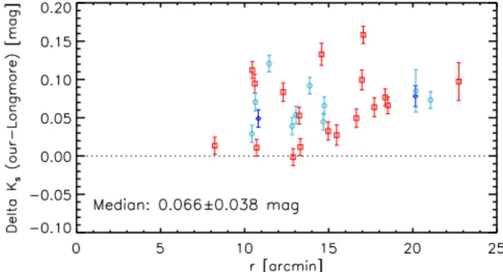
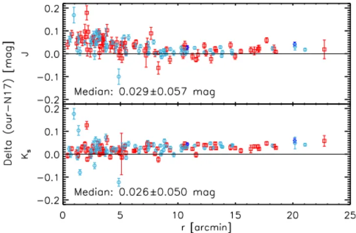
3.3. Mean Magnitudes and Amplitudes
In the literature, the sampling of NIR light curves of variable stars is far from being ideal. This is the main reason why template light curves have been developed for both RRLs(Jones et al.1996) and classical Cepheids (Soszyński et al.2005; Inno et al.2015). The phase coverage of the current data set is quite
good and ranges from around 10 to 60 measurements per band. However, for variables located in the outskirts of the cluster (four RRLs between 20′ and 32′ from the center of the cluster) we have less than 10 measurements. For an additional 16 RRL candidates farther away, we have only retrieved one measure-ment from both VHS(JKs, McMahon et al.2013) and 2MASS
(H, Skrutskie et al. 2006). In order to quantify the impact that
analyticalfits of the light curves have on the mean magnitudes and on the photometric amplitudes we decided to use three different approaches.
Locally weighted polynomial regression, PLOESS. A similar method (GLOESS) has already been applied to fit randomly sampled light curves (Persson et al.2004; Neeley et al.2015; Monson et al. 2017). The key idea of this approach is to
provide a plausible guess of thefitting function in a phase range for which the sampling is either too coarse or too noisy to allow fitting a low-degree polynomial to a subset of the data. Moreover, to limit the contribution of possible outliers, the individual points are weighted with a weight function. This is the reason why PLOESS is a local weighted regression method. The algorithm we developed relies on the following steps. Let us assume that the time series data of the variable we are dealing with consists of xi (phase), yi (magnitude) data with
i=1, K, n phase points. The original data are divided into subsamples, each one including≈20%–30% of the entire data set. Moreover, the weights for the individual data points in the subsample are defined using the following formula:
Wi=(1-abs([X-xi] DX) )3 3
where X is the phase at which we would like to have a new smoothed value along the light curve, xi are the data in the
subsample andΔX is the maximum distance in phase between X and the data in the subsample. The weights were defined in such a way that the data point to be smoothed (X) has the largest weight. The weights (Wi) of the data points in the
subsample(xi) decrease as a function of their distance from X,
while the data points not included in the subsample have zero weight. The weighted least-squares regression on the data of the subsample is performed using a second-degree polynomial and provides a new value of the light curve at the phase of the data point (X) we are smoothing. To overcome the typical problems at the boundaries of the phase interval[0, 1], the data points were triplicated, i.e., the smoothing was performed on data replicated over the phase interval[−1, 2]. Moreover, the data points included in each subsample are symmetric, i.e., the number of data points to the left and to the right of the data point (X) is always the same. We performed a number of simulations using also the weight function suggested by Cleveland (1979), but we found that the current weight
function provides smoother light curves when the original data points are grouped in restricted phase intervals. Finally, to further improve the stability of the fit, we also computed the residuals of the original data points from the smoothed light curve and, using an iterative procedure, we neglected from the smoothing the data points that are located at a distance larger than six times the median absolute value.25
Spline. This is a classical approach with the key advantage of tightlyfitting the data points. However, this approach is more prone to systematic errors when the time series data are either unevenly sampled or characterized by significantly different random errors. The splinefits, too, were derived on a triplicated light curve with phases in the interval[0, 3] to avoid boundary effects. We adopted the middle section—phases in the interval [1, 2]—of the spline fit as the final fit of the light curve.
The two quoted approaches were adopted to fit J-, H- and Ks-band light curves. The PLOESS approach was adopted only
for light curves with a number of phase points larger than nine. Template. The Ks-band light curves were also fit with the
template light curves provided by Jones et al.(1996). We found
that, for more than 60% of the light curves in our sample, the mean magnitudes based on the template fit are, within the uncertainties, very similar to those based on the spline and on the PLOESSfit. However, this method is extremely sensitive to the accuracy of the period, to possible period variations, and to phase modulations (mixed-mode, Blazhko). Indeed, for more than∼35% of RRL candidates we found a phase shift between the template light curve and the observed data points. To overcome this limitation we adopted a different approach to apply the templatefit. The first two steps are the same as in Jones et al. (1996): first, we selected the template based on the
pulsation mode and on the optical AB(or AV ) amplitude; second, we set the scaling factor of the templatefit as half of the Ks-band
amplitude, calculated as AKs =0.108·AB +0.168mag (RRab) and AKs=0.110 (RRc). The third step—the phasing
of the template—is different: instead of anchoring the template to one of the phase points—as in the canonical template fit—we
25This algorithm was implemented in IDL and it is available upon request to the authors.
11
minimized the residuals(χ2) using two free parameters: the mean magnitude and the phase shift. Note that to further improve the accuracy of the fit we could have used the AKs amplitudes
evaluated using either the spline or the PLOESSfit. We followed the classical approach to test both the accuracy and the precision
of the template light curves. The above findings call for the development of new template light curves, and in particular for extension of the template light curves to the J and H bands. Figure6shows the light curves in the JHKsbands of an RRc and
an RRab variable with good phase coverage. Spline, PLOESS,
Figure 6.Top: light curve for the RRab variable V44. The red line shows the splinefit, while the blue line the PLOESS fit and the green line the template fit. The vertical error bars display the intrinsic photometric error. The name and the period of the variable are labelled in the top-left panel. In the top-left corner of each panel, thefitting model (spline, PLOESS) that was selected as the best one, is labelled. Bottom: same as the top, but for the RRc variable V105.
Figure 7.Top: same as the top in Figure6, but for the RRab variable V59. Bottom: same as the top, but for the RRab variable V130.
12