AUTONOMOUS PROVINCE OF TRENTO
Provincial Environmental Protection Agency
LAKE SHOREZONE FUNCTIONALITY
INDEX (SFI)
A tool for the definition of ecological quality as indicated by Directive 2000/60/CE
Maurizio Siligardi (coordinator)
Serena Bernabei, Cristina Cappelletti, Francesca Ciutti, Valentina Dallafior, Antonio Dalmiglio, Claudio Fabiani, Laura Mancini, Catia Monauni, Sabrina Pozzi, Michele Scardi, Lorenzo Tancioni, Barbara Zennaro
INDEX
1. Introduction………... 5
2. Lake shore environments and Water Framework Directive……… 7
3. Ecology and function of the lake shore zone……….9
4. Shorezone Functionality Index: introduction……….………….14
4.1 Methodology……….………14
4.2 Characterization of the “classification trees”……….………...16
4.3 Development of the SFI card……….………..17
5. Shorezone Functionality Index (SFI): protocol……….……….19
5.1 Preliminary Investigation……….19
5.2 Survey form for the SFI parameters……….18
5.3 Sampling methodology………..25
5.4 Calculation of lake shore functionality levels………27
5.5 Levels and functionality maps………31
6. How to fill out the field form………33
6.1 Width of the lakeshore zone………35
6.2 Characterization of the lake shore zone vegetation………….38
6.2.1 Composition/cover……….39
6.2.2 Hygrophilous and non hygrophilous Vegetation…..41
6.2.3 Presence of exotic specie……….42
6.2.4 Heterogeneousness of arboreal and shrub vegetation..44
6.3 Continuity of lakeshore vegetation………...47
6.4 Presence of interruption within the lakeshore zone…………48
6.5 Typology of anthropic use within the lakeshore zone……….50
6.6 Prevalent use of surrounding area……….51
6.7 Infrastructure………53
6.8 Emerged lakeshore zone………57
6.8.1 Average slope……….57
6.8.2 Slope comparison between emerged and submerged lakeshore area……….58
6.9 Shore profile………..………60
6.9.1 Concavity and convexity……….60
6.9.2 Complexity……….…….62
6.10 Shore artificiality………..66
6.11 Apparent channelling of run-off………....67
7. Lakeshore Functionality and naturalness……….71
8. Ending remarks………. 73
9. Bibliography……… 74
Acknowledgements………80
1. Introduction
The international literature offers a vast bibliography on riparian fluvial areas, including numerous contributions on vegetation and fauna, on ecological function, re-naturalization and reclamation of the buffer strip, on the planning value, consolidation actions and so on (Vidon & Hill, 2006; Hatterman et al., 2006; Naiman & Decamps, 1997; Naiman et al., 1993). Although, studies on the role of the lake’s riparian area are often only poorly and marginally treated (Keddy & Fraser, 1983, 1984, 2000; Zhao et al., 2003; Hazelet et al., 2005; Marburg et al., 2006; Hwang et al., 2007; Ostojic et al., 2007).
The coastal habitats have many natural elements interlinked with the lake ecosystem to form an ecological web. For example, the vegetation, the sediments and the detritus play an important role in the vital cycles of fish and coastal fauna (McDonald et al., 2006; Dudgeon et al., 2006; Malm Renofalt et al., 2005).
The lakes are affected by the chemicals coming from the watershed’s streams, that, like in the case of nitrogen and phosphorus, affect actively (and often negatively) the trophic-evolutionary processes of their waters. (Premazzi & Chiaudani, 1992; Chapman, 1996).……… To date, classic limnology studies failed to focus on the simple functionality of the lake riparian zones.
The riparian zone has an important role in protecting and buffering the degradation of the aquatic ecosystem derived by human activities (Cobourn, 2006). Land uses that consisted in the elimination of riparian vegetation, often caused environmental stresses, increased instances of no-point source pollution, and resulted in morphologic alterations and habitat destruction (Schultz et al. 1993, 1995).
Studies by Osborne and Kovacic (1993) have shown that the riparian zone, (both herbaceous or shrub/arboreal types), can efficiently intercept the nutrients coming from nearby agricultural areas, diminishing by over 90% the nitrogen and phosphorus contents in both superficial and sub-superfical waters flowing into the water body.
There are many and dissimilar interests on the lake’s environments. For example, the waterfront owners often see the lake shorezone as a resource to be exploited: a lake, beside having a great naturalistic value, also guarantees numerous opportunities for water activities, such as swimming and aesthetic satisfaction, which can be exalted by proper lake ecosystem management and protection policies.
Such vision requires a the creation of a system of indicators, and thus indices, that are able to support and guide land planning policies and management choices. Following the success of the IFF (Index of Fluvial Functionality – Siligardi et al., 2007), a new model was created in order to been able to calibrate the efficiency of the lake shore zone, using biotic and abiotic descriptors that are easily surveyed (Broocks et al., 1991; Keddy & Fraser, 2000; Lin et al., 2000; Dale & Beyele, 2001; Danz et al., 2005; Brazner et al., 2007). The need for a new index was also supported by the request of the Water Framework Directive 2000/60/CE that, to define the ecological quality state, places side by side the evaluations of biological elements with the evaluation of hydro-morphological elements.
2. The lake shore environments and the Water Framework Directive 2000/60/CE
The Water Framework Directive (WFD) 2000/60/CE defines the elements of quality (EQ) to classify the ecological state of water bodies of any typology. Among the EQ to be determined, there are biological elements and hydro-morphological elements which, for lakes, consist in the hydrological regime (quantity and dynamics of the water flow, water percolation, and residence time) and the lake morphology (variation of depth, substrate’s characteristics and shore’s structure) (CIS, 2003). Concerning the lake-shore-zone, the document “The Horizontal Guidance Document on the Role of Wetlands” contained in the framework directive (CIS wetlands WG 2003) is the most important reference to article 1 of the Water Framework Directive in which the wetlands are described as depending directly on the ecosystem of internal superficial water bodies (such as lakes).
The ecosystem of the lake-shore-zone located the closest to the water is commonly called wetland: this is an area with a characteristic lakeshore ecotone, with a gradient going from the surrounding land to the aquatic environment and that varies with periodic changes in water levels (including flooding). In the CIS document the lake-shore-zone is clearly associated to the wetlands, sensu Directive, and nevertheless it is consider as an integral part of the lake, able to influence the related ecological status. Consequently, diverse water-related WFD objectives and obligations do consider the lake-shore-zone as well (CIS Wetlands WG 2003, page 10 to 13).
However, the Directive does not provide for wetland’s environmental objectives and for such reason, at the Copenhagen’s meeting on November 2002, the Member States defined that tampering the shorezone is an environmental impacting act for the ecological state of the water body. Thus, wetland or, in our case, shorezone management is considered an integral part of the Basin Plans and the conservation and extension of wetlands and lake-shore-zones may be the instrument to reach the WFD objectives. These considerations have been acknowledged by the CEN Technical Committee 230/WG2 “Water Analysis” and by Member States and others such as Switzerland.
The looking into the different methods used by the Member States immediately showed the absence of standard and consistent methods in the EU.
Definite EQ and measurement program to be included in the Plans of the water management for each hydrogeographical District, were needed to reach the environmental objectives defined by the WFD on environmental protection policy and sustainable use of the water bodies.
The hydro-morphological quality elements are of fundamental importance in the analysis of water bodies, in particular those classified as highly modified (HMWB) or artificial, that risk not to reach the environmental objectives required by the Italian government Basin Programs.
……….
It is therefore very important to develop and apply indices such SFI (or the similar IFF for rivers) since they offer an answer on the state and ecological potential of a water body (lake, river), regarding as well the hydro-morphological aspects.
3. The lake shore-zone: ecology and function
The “lake shore-zone” extends around the lake with a defined width and has various ecological functions which depend on many environmental factors.……….
The morphology and characteristics of the lake shores are very important being functional elements for the ecological dynamics of the water bodies and for its biodiversity. The morphological characters, apparently not influential on the qualitative processes, are very important in evaluating the functionality of the coastal areas.…Moreover, even the topography of the land surrounding the lake influences land-lake exchanges: the greater is the geometric complexity of the lakeshore profile, the minor is the nutrient input derived by limnological processes, since the geometric complexity reduces the content of BOD, COD and TP (Hwang, 2007).
The lake-shore riparian ecosystem, even if less obviously than the fluvial one, guarantees a conspicuous supply of water that contributes to the growth and survival of plants, insects, animals and microorganisms, therefore increasing biodiversity and consequentially functionality (Giller, et al., 2004). Plants constitute an element of structural and taxonomic diversity and are able to moderate seasonal water flows by storing water and by regulating the amounts of sediment and nutrients inputs (Smith and Hellmund, 1993).
Topography, climate and the soil geological composition greatly influence the structure and extension of the lake shore-zone. Likewise, the lake shore-zone vegetation controls considerably the water flow, nutrients and sediments inputs, and the diffusion of animals and plants towards the lake from the surrounding area (Malanson, 1993b; Naiman et.al., 1993). Different amounts of nutrients are derived on the diverse land uses, which could be agricultural, industrial, urban, uncultivated or other.
The vegetation strip along lake is therefore considered a transition zone between the surrounding area and the water body in both a topographic and functional point of view (Pinay et al., 1990; Smith & Hellmund, 1993; Malanson, 1993b; Vidon & Hill, 2006; Hazelet et al., 2005) and it plays an important role in shore protection (Maynard & Wilcox, 1997; Ostendorp, 1993) Maintaining an healthy vegetated lake shore-zone is important as it intercepts the waters (both superficial and subterranean) coming from the surrounding watersheds that carries nutrients that would otherwise enter into the lake without obstacles (Burt et al., 2002; Van Geest et al., 2003).
It is also very important that area close by the shore, where the macrophytes are at the base of the trophic web. The biodiversity of the macrophyte community
depends on the variation of factors such as depth, water level fluctuation, granulotory and exposure to the waves (Keddy & Reznicek, 1986; Keddy, 1990; Ostendorp, 1991; Wilcox & Meeker, 1992).
Besides these ecological functions, the lake shore has also a human recreational function, by being highly attractive to tourists (Bragg et al., 2003; Wilcox, 1995).
The following definitions are used by the SFI for the different portions of the Lakeshore zone:
- Shoreline: the line on the shore where water and soil make a contact. This portion can be bare, herbaceous or have a more complex vegetation such as stumps, logs, branches, root systems, bed of reeds or other;
- Littoral zone: the section of the lake along the shore in correspondence to the euphotic (well illuminated) zone which generally coincides with the limit of presence of submerged macrophytes; it often hosts phytobenthic and zoobenthos communities and it is a refuge for many aquatic and non-aquatic animals. Many fish species choose this area for eggs deposition and development (Baker, 1990; Doyle, 1990; Pollock et al., 1998; Bratli et al., 1999; Wetzel, 2001; Roth et al., 2007);
- Riparian zone: the land area immediately adjacent to the lake with ecotonal functions that is formed by both terrestrial and aquatic habitats and that guarantees an high level of biodiversity (Wetzel, 2001). It can significantly affect the quality determined by other hydro-morphological, biological or physical elements and in return can be influenced by flooding and wave action.
- Lakeside zone: the land portion that interacts with the lake environment; it does not have an ecotonal structure and/or function but it is mainly a terrestrial environment.
The scientific community lacks a general agreement to indicate and define the ecologically functional strip, and expressions such as the ones describes above (lakeside zone, riparian zone, littoral zone and shoreline) do not completely reflect the significance of the ecotonal zone. For example, while for the CIS Wetlands Group (CIS, 2003) the word “shorezone” describes the littoral zone,
especially for natural lakes, other scientists define it differently, giving to it a stronger stress on its ecological functions rather then on its geographic and morphologic characteristics (Schmeider, 2004).
The word “lake-shore”, lately used in literature to indicate that area with a morphological and functional role of ecotone, includes both the littoral zone and the riparian zone (Ostendorp et al., 2004) (figure 1).
Therefore, the term “lakeshore” is used here to indicate the transitional area (ecotone) that links the terrestrial environment to the pelagic one (Naiman & Decamps, 1997)
By “lake-shore-zone” it is meant the topographical strip situated around the lake that includes part of the littoral zone (up to a maximum depth of 1 m) and the strip of land that extends up to 50 m from the shoreline.
fascia litoranea fascia riparia territorio circostante linea di costa fascia perilacuale
Figure 1 - scheme of the different lake-shore-zones
The natural lake-shores can have different characteristics that depend on the vegetation and geology, genesis, age, depth and lake shape, geomorphological processes, sedimentation delta, wave action and water level changes.
Lake-shores have an ecotone role, separating and simultaneously relating the terrestrial and the aquatic habitats, regulating their sink-source fluxes (Farina,
Lake Shore Zone
Surrounding Land Riparian Zone
Littoral Zone Shore
2001). In fact, they work as filters able to tampon and depurate waters (littoral and riparian) rich in nutrients (Hatterman et al., 2006; Cirmo & McDonnell, 1997; Krysanova & Becker, 2000; Lin et al., 2002).
The lake-shore-zone is quite important for the different functions that it has for the lake ecosystem:
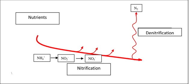
1) Filter: the rain and run-off are slowed down by the vegetation that facilitate the infiltration, sedimentation and pollutant capture (Pinay et al., 1990) (Fig. 2).
2) Erosion protection –the tree roots retain the lake-shore soil preventing or reducing the erosion processes caused by the natural action of waves or induced by swimmers (Heckman, 1984).
3) Nutrients removal – nutrients, such as the nitrogen or the phosphorus coming from the surrounding watersheds, can be intercepted by the root systems of the lakeshore zone vegetation, metabolized and stored in leaves, trunks, and roots (Pinay et al., 1990; Vanek, 1991; Vought et al., 1993, 1994; Shultz et al., 1995; Push et al., 1998). Phosphorus is the main limiting nutrient in lakes and can favor eutrophication processes in lake waters. Its removal can occur by three different solutions:
a) deposition in lake sediment;
b) absorption and sink of dissolved phosphorus (i.e. orthophosphate) in bottom sediment particles (Triska et al., 1993; Vought, 1993);
c) uptake of nitrogen and soluble orthophosphate by suction operated by the root apparatus of the lakeshore zone vegetation (Vought, 1993, 1994) (Fig. 2).
The efficiency of the tampon zone changes with the different seasons, when duration and intensity of the water fluxes vary; for example, a lake-shore-zone vegetation composed by deciduous plants has an higher filter efficiency and nutrients removal capacity during the vegetative period
(spring-early fall) than during physiological dormancy (late fall-winter) (Mitsch & Grosselink, 1986).
4) Temperature control – The shade produced by the tree foliage attenuates the solar irradiation, controlling the water temperature along the coast, where often the fauna settles and egg deposition occurs ( Gregory et al., 1991).
5) Habitat – The vegetated lake-shore-zone furnishes an ideal habitat for many species of animals (fish, amphibians, reptiles, birds, mammals, insects, etc.) offering refuges and the food necessary for survival and reproduction (Callow and Petts 1994). It is particularly important for fish habitat and it is therefore an element that need to be protected when aiming to the maintenance of the fishing resource.
6) Anthropic value - A healthy vegetated lake-shore-zone is important for naturalistic and aesthetic points of views. Sometimes it also have cultural, historical and archaeological reasons when historically importance.
Figure 2 - Representation of the tampon function of the lake-shore-zone \ nitrificazione denitrificazione NH4 + NO2- NO3 -nutrienti N2 Nutrients Nitrification Denitrification
4. Shore-zone Functionality Index (SFI): introduction
4.1 Methodological approach
A work group was officially instituted by APAT, now ISPRA, to create a new method able to satisfy the necessity of indices for the evaluation of the functionality of the lake-shore-zones.
After a first classic approach based on consolidated experience of the IFF ( Fluvial Functioning Index ) (Siligardi et al., 2007), the work group, wanting to include bioindicators and new available technologies, included in model Machine learning, artificial intelligence and fuzzy logic, as inspirations of the new ecosystem vision.
Only two approaches are possible when evaluating the functionality of an important ecological structure, the integrity of a community, or other characteristics of closely related entities:
• The first approach consists in the recognition of the recurring typologies and their successive interpretation with the attribution a posteriori judgment (a quality score or a classification value –which is not based on a scheme that distinguishes what is desirable from what is not). This approach was used for the development of the CAM algorithm (Classification of Marine Waters), adopted to evaluate the data from the coastal marine water monitoring program (coordinated by the Environment Departement -www.minambiente.it).
• The second approach consists in the a priori evaluation of the quality and the functionality of the observed parameters, done during field work by technicians. Practically, a personal judgment is given to the different parameters surveyed. Afterwards, this information is entered into a database and used to run the SFI model based on a classification tree.
After trying different explorative techniques (as ordinance and hierarchy classifications) and self organizing maps, an approach based on the classification tree was adopted to treat the data collected to create a
Shorezone Functionality Index, after trying different others traditional techniques, such as Hierarchic classification, neural net analysis (Self Organizing Maps), and modern analysis such as Machine Learning (Scardi et. al., 2008). For an introduction to the ecological applications of the method please refer to Fielding (1999).
The classification tree allows to link unequivocally a set of observations on the structure of the lake-shore-zone to an evaluation of its potential functionality, in other words, its apparent capacity to protect the water body from the no-points-source inputs coming from the adjacent watersheds.
Ecologists and naturalists can easily understand the method, as it generates a binary tree that has the same structure as the dichotomic tree used to identify species.
The solution, which is not the only possible or necessary the most efficient, was chosen because it was considered optimal considering the explorative nature of the work completed. In particular, the main objective was to elaborate an easily applicable method that functioned on rather limited set of field observations. The workgroup therefore created a field form to collect the largest number of parameters and indicators to identify the most significant information for the proposed objectives.
The form is divided into three groups of parameters: 1) general parameters a) topographical b) morphological c) climactic d) geological e) others 2) ecological parameters a) vegetation type b) size c) continuity d) interruption
3) socio-economical parameters a) general b) land use c) infrastructure d) tourism e) tourist infrastructure f) productive activities
4.2 Characteristics of the classification trees
A classification tree is a binary tree that represents a group of rules that are applied to classify multi-variate observations. Each classification tree’ s “leaf” represents a more or less frequent type of observation and more leaves can belong to the same class; therefore these can be considered as a subgroup of the classes recognized by the system.
Once organized, the classification trees can be used to classify objects or observations following sequentially the rules associated to each tree’s fork, until reaching the leaves.
These can be more or less pure, depending whenever or not they contain objects and observations classified in an incorrect way. Generally, obtaining pure leaves implies a reduced capacity to generalize the tree (overfitting). In other words, if the tree overfits defined existing cases used for its creation, the generated rules are associated too closely to these particular cases and became useless when other slightly different cases must be classified. On the contrary, if the tree structure and the rules that it contains are simple, the probability that the tree is efficient even when classifying new cases, increases. For this reason, in many cases, the tree is “trimmed” once developed, with the goal to reduce its complexity and to increase, whenever possible, its generalization capacity.
Among all the Machine Learning techniques, the classification tree is the one that can be used more easily by a general public. In fact, the complexity of the algorithms that are used to run the trees is completely transparent to the final user and to the developer.
In particular, among the advantages of a classification tree, the following are important:
• they are easy to put together, since algorithms are generally efficient and tested (e.g. C4.5, ID3, CHAID, etc.) and able to autonomously estimate the optimal structural parameters for a tree;
• they are easily understood, graphically represented and interpreted, unlike other machine learning techniques such as artificial neural nets and non-linear regressive models;
• their practical application does not require calculations of any type but only the verification of a group of simple logical conditions;
• they can manage efficiently both quantitative variables and semi-quantitative or nominal variables, while other methods do not always treat efficiently the latter;
• they are particularly efficient in managing cases of interactions between variables, which are resolved by appropriately partitioning the defined space of the considered parameters;
• they can suggest which parameters are more important in determining the classification; this does not require any added analysis but only a visual inspection of the tree structure.
4.3 Development of the SFI survey form
The SFI form and its parameters were defined between 2004-2009 in a series of attempts which began with the identification of a wide range of parameters that could be associated to the lake-shore-zone functionality. The first group of parameters were narrowed after using the preliminary form on some lakes: this process brought to the elimination of those parameters that resulted pompous and insignificant.
The parameters were also selected on the basis of their easily availability for all types of lakes; for example meteoclimatic information was excluded because not always available.
The initial use of an “experimental form” made it possible to evaluate the difficulties of compiling it, to better define the required parameters and to improve the methodology in assigning scores. Through field work, it was also possible to make a preliminary protocol for the correct interpretation of the form. The SFI parameters, latter described in this book, were defined during this first phase.
5. Shore-zone Functionality Index (SFI): protocol
5.1 Preliminary Investigations
It is important to do a preliminary investigation before going out in the field in order to have a basic understanding of the environment to be surveyed. Maps of the lake and the surrounding environment are therefore useful to have a perspective of the lake in its entirety, to investigate land uses, to identify roads and access points to the river. These maps will also be used in the field to annotate the location of the homogeneous stretches found.
Useful information for thematic maps includes: vegetation, land use, soil type, altitude, bathymetry, aerial photos, etc. A scale of at least 1:10,000 is recommended for the fieldwork, as it provides a certain amount of details necessary for the environmental analysis.
It is also advisable to use aerial photography to complement the thematic maps.
5.2 Survey forms for the SFI parameters
The parameters considered useful for the determination of the SFI are collected into a “field card”, subdivided into two different forms. The first form is about the lake in general while the second form contains information about the ecological and morphological characteristic of each homogeneous stretch found in the field.
The homogeneous stretch is identified in the field through direct observation and with the aid of the maps created during the preliminary analysis.
The place where shore-zone clearly changes, especially changes regarding the human impact’s weight (i.e. artificiality of the shore-zone) or the shore-zone vegetation structure (i.e. composition, width…), indicates the end of an homogeneous stretch and the start of a new one. In this case, a new form is filled for the new stretch.
There is not a pre-established length to be used for the homogeneous stretch, which could be kilometers long, but it must be at least equal or superior to the Minimal Detectable Stretch (MDS). The size of the MDS depends on the size of the lake, the weight of anthropic impacts, the structure and shape of the lake shore-zone, etc.
Generally, in the case of large lakes (perimeter above 50 km), the minimum stretch to be sampled cannot be less than 200 meters, with the exception of stretches with particular characteristics or anthropic impacts that would require the filling out of another card.
The information requested for the first form (Table 1) is gained from cartographic, bibliographical, or monitoring campaigns sources. This information is not used when assigning the SFI value, but is important for the general knowledge and understanding of the lake structure.
INDICATOR Parameter expression typology
origin1 - category type2 - category location3 - category latitude degree, minutes, seconds number longitude degree, minutes, seconds number
altitude of lake meters asl number
TOPOGRAPHICAL
average altitude of catch basin meters asl number area of catch basin (SB) km2 number shore slope degree or percent number development of shore line - number
area of lake (SL) km2 number
volume Km3 number
maximum depth meters number
average depth meters number
average residence time years number tributary/effluent capacity m3/second number
SB/SL relationship - number
MORPHOLOGICAL
level changes - presence/absence
precipitation mm/year number
average maximum Jan. temp. degree centigrade number
CLIMATIC
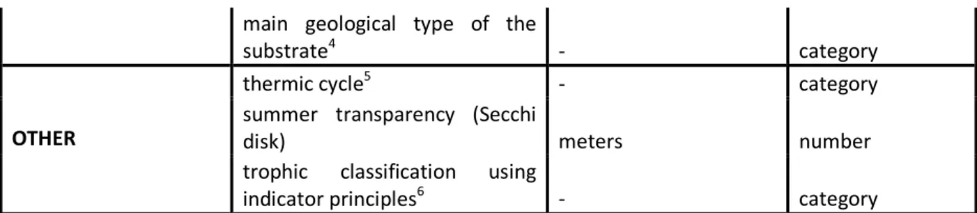
main geological type of the
substrate4 - category
thermic cycle5 - category
summer transparency (Secchi
disk) meters number
OTHER
trophic classification using
indicator principles6 - category
¹= tectonic, volcanic, glacial, oxbow lake, landslide, endorheic, coastal, seasonal, other ²= artificial, open natural, natural large, natural closed, natural regulated, other ³= alpine (mountain), pre-alpine (half mountain), lowland
4= calcareous, magma, metamorphic, sedimentary, other
5 = holomitic, monomitic, dimitic, polymitic, meromitic, amitic, other
6 = ultraoligotrophic, oligotrophic, mesotrophic, eutrophic, hypertrophic
Table 1 - First part of IFP card: general data
The second form refers to the conditions of each single homogeneous stretch of the lake shore-zone, considering the parameters showed in the following table. (Table 2).
Tab. 2 – Useful parameters for the SFI with indications of the typology and evaluation.
Parameter Typology Value Notes
1 width of lake shore-zone category 0,1,2,3,4,5 2 characterization of lake-shore vegetation
2.1 cover/composition % numerical
% - from 0 to
1 Σ = 1 except in particular cases
2.2 hygrophilous and non-hygrophilous vegetation numerical
% - from 0 to 1 Σ = 1
2.3 exotic species presence numerical
% - from 0 to
1
2.4 heterogeneous arboreal-bush vegetation numerical from 0 to 1 3 continuity of lakeshore vegetation category 0, 0.5, 1 4 interruption within lake shore-zone numerical from 0 to 1 5 typology of anthropic uses in lake-shore-zone category 0, 0.5, 1 6 main use of surrounding land category 0, 1,2,3 7 infrastructure numerical from 0 to 1 8 emerged lake-shore-zone numerical 8.1 average slope category 0,1,2,3,4,5 8.2 slope comparison between emerged/submerged areas category 0,1 9 shoreline profile numerical 9.1 concavity and convexity numerical from 0 to 1 9.2 complexity numerical from 0 to 1 10 shoreline artificiality numerical from 0 to 1 11 apparent channeling of run-off category 0, 0.5, 1 12 personal judgment category 0,1,2,3,4,5
All the information necessary to fill the form are collected in the field, using Table 3. The methodology to express each parameter is specified each time.
It was decided to use a scale based on numerical scores for facilitate the statistical elaboration; the scores were chosen considering a range of values that estimate the different weight of each parameter.
As it is described in the methodology section, not all parameters will be part of the resolution set and identification of level of functionality; however, it is opportune to fill out the form in its entirety to have a complete inventory of the characteristics of the lake shore-zone that allows other possible elaboration and that can be used in planning and management projects.
It is also possible that (as often happens with any qualitative or semi-qualitative indexes based on heuristic processes and fuzzy logic) the application will be re-calibrated few years from now.
Date Lake Form Number Delimitation of stretch Photograph number Surveyors GPS coordinate Lake shore-zone
The boundary of the lake shore-zone is determined by ………..
1. width of lake shore-zone
0 m 0 1-5m 1 5-10m 2 10-30m 3 30-50m 4 >50m 5
2. characterization of lake-shore-zone vegetation
2.1 cover/composition % (expressed from 0-1)
trees %
reeds%
grasses%
bare soil%
2.2 Hygrophilous and non-hygrophilous vegetation (expressed from 0-1) hygrophilous (helophytes, riparian shrub and riparian arboreal species)
non-hygrophilous (other species)
2.3 Presence of exotic species (expressed from 0-1)
exotics %
2.4 Heterogeneousness of arboreal-shrub vegetation
diversified 1
intermediate 0.9-0.7
monospecific 0.6
autochthonous hygrophilous arboreal-shrub species >2/3
diversified 0.5
intermediate 0.4-0.3
monospecific 0.2
autochthonous hygrophilous shrub species < 2/3 and autochthonous
arboreal-shrub < 2/3
autochthonous relevance 0.1
exotic prevalence 0
arboreal-shrub vegetation absent 0
3. Continuity of the lake-shore vegetation
arboreal and shrub zone
absent 0
discontinuous 0.5
continuous 1
wet reed zone
absent 0
discontinuous 0.5
continuous 1
dry reed area
absent 0
discontinuous 0.5
continuous 1
4. Presence of interruption on the lake-shore zone
absent 0
intermediate
present along the whole stretch 1
5. Typology of anthropic uses within the lakes-shore zone
uncultivated meadows or unpaved streets, etc. 0
sparse urbanized, cultivated meadows, etc 0.5
SHORE AND SURROUNDING TERRITORY
6. Main Use of nearby territory
woods and forest 0
meadows, forests, arable land, uncoltivated 1
seasonal cultures and/or permanent ones and sparse urbanization 2
urbanized area 3 7. Infrastructure Provincial/state roads absent 0 intermediate
present along the whole stretch 1
Railroads
absent 0
intermediate
present along the whole stretch 1
Parking
absent 0
intermediate
present along the whole stretch 1
Tourism related infrastructure
absent 0
intermediate
present along the whole stretch 1
8. Emerged portion of lakeshore zone
8.1 average slope
flat 0
slightly noticeable slope 1
obvious but can be overcome without problems 2
significant but can be overcome with trails or ramps 3
strong slope, roads or trials with bends 4
extreme, vehicles cannot drive 5
8.2 comparison between slope of emerged and submerged area
not consistent 0
consistent 1
9. Shore profile
concavity
absent 0
intermediate
present along the whole stretch 1
convexity
absent 0
intermediate
present along the whole stretch 1
9.2 complexity
absent 0
intermediate
present along the whole stretch 1
10. Shoreline artificiality
absent 0
intermediate
present along the whole stretch 1
11. Apparent channeling of run-off
no prevalent direction for the flow 0
intermediate
all the run-off converges in a single point 1
12. Personal judgment excellent 1 good 2 average 3 below average 4 very bad 5
Table 3 - Parts 1and 2 of the SFI form to be used in the field
5.3 Sampling methodology
The data collection for the entire lake (Part 1) can precede the field inspection.
The filling out of Form 2 is done exclusively in the field, with different forms referring to different homogeneous stretches. As soon as a “significant change” occurs, even in only one of the sampled parameters, a successive homogeneous
By “significant change” is meant the any significant change of one or more of the parameters, for example: changes in the width or typology of the lakeshore zone, changes in the presence of infrastructure or interruptions that are absent in the previous stretch, changes in complexity or artificiality of the shore, etc. Changes in the concavity and/or convexity parameter are often not enough to decide to compile a new form if all the other parameters remain constant. In the case of shorelines with frequent depressions and inlets, it is better to take into consideration the surveying scale (and therefore the length of the minimum stretch length to be sampled), to make an adequate stretches subdivision.
For practical and safety reasons, it is also advisable to have at least two people doing the survey, which also guarantees a reciprocal scientific validation.
The form should be compiled walking along the shore of the monitored stretch. The fieldwork should be done during the vegetative season as information regarding the lakeshore zone vegetation is requested. In the case of steep stretches or stretches with dense shore vegetation, for which access by foot is difficult, it is recommended to go along the lake with a boat to survey possible vegetation interruptions and natural or artificial shore condition.
It is useful to take photographs during the field work that can be linked to the filled form. For a more precise delimitation of the stretches, it is recommended to use the GPS to register the stretch’s starting and ending point coordinates. GPS lines are also very important to import the data into a GIS database, which can greatly enhance cartographic representation and spatial analysis.
The necessary material for the application of the method consists of:
- trekking clothing and adequate personal safety equipment - maps scale 1:10,000 of the lake
- orthophoto maps (aerial maps geometrically corrected to have an uniform scale)
- an adequate number of forms to be filled out - digital camera
- pencils and erasers
- paper to note things of particular interest - metric cord
- fishing boots
- optic telemeter laser (advisable) - GPS
Tablet PC with incorporated GPS are very useful to directly geo-reference the stretches and to mark them on a digitalized technical card. This kind of data can be easily downloaded, re-organized, and elaborated.
5.4 The approach
The application of the classification tree to the data regarding the parameters of the shore zone of different lakes (for a total of 450 forms collected) allowed to draft a first hypothesis on the evaluation of the slake shore zone functionality.
The use of the classification tree was then made simpler by a Windows platform that requires only the data relative to the essential descriptors. In the list of the parameters considered by the classification tree to evaluate the lake shore zone functionality, only 9 resulted being decisive to classify each stretch:
o Shore artificiality o Vegetation cover
o Interruption of the lake-shore-zone o Concavity of the shore profile o Reeds presence
o Arboreal species presence o Road Infrastructure
o Heterogeneity of arboreal vegetation o Non-hygrophilous species presence
It should be specified that even the information regarding the parameters not included in the actual classification tree is anyway useful as they compose a database of the morphological and ecological characteristics of the lake-shore-zone, some of which correspond to the qualitative elements required for the classification of the ecological state of lakes (EC Directive 2000/60/CE).
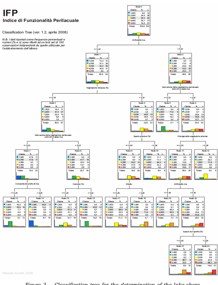
Figure 3 shows the classification tree used. There can be different pathways throughout the classification tree depending on the values given to the parameters.
For each leaf and node, the probabilities of falling in any of the functionality classes are signed, 1 being excellent and 5 being very bad. The grey underlined line in the table representing each leaf and node, represent the most probable class.
When classifying a stretch of lake shore, the first parameter that is verified (at the root located on the top on the classification tree figure) is the degree of artificiality of the shore (either <0.22 or >0.22). From here, the next parameter that will evaluate the functionality level is the vegetation and the environmental fragmentation.
Figure 3 - Classification tree for the determination of the lake-shore levels of functionality with the relative percentages.
The SFI software calculates directly, for each stretch, the functionality level and the probability of being assigned to each of the level.
For this reason, it is important to emphasize how some attributes are considered more than once in different parts of the tree (i.e.. % grasses). This also reflects an optimal use of all the information available.
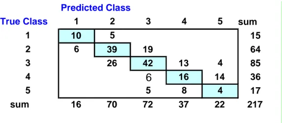
The Cohn test (Cohen, 1960) was carried out to check the correlation level between the results obtained through direct observation (based on expert judgment) and the outcome modeled by the application, (table 4).
Table 4 - Agreement of the theoretic results, derived from the application of the model, and the ones based on personal judgment.
The results showed a K value of 0.673 (p<0.01), meaning that the results obtained though direct observation resulted to be substantially similar to those obtained through the model (Landis & Koch, 1977). The 51.2% of the cases were estimated correctly, and the 95.9% of the cases were estimated with an error of only one functionality level. Therefore, only a 4.1% of the cases had an error above this margin and these errors were anyway relative only to classes 3, 4 and 5.
Predicted Class
True Class 1 2 3 4 5 sum
1 10 5 15 2 6 39 19 64 3 26 42 13 4 85 4
6
16 14 36 5 5 8 4 17 sum 16 70 72 37 22 2175.5 Levels and Functionality maps
The final score is divided into 5 functionality levels, expressed in Roman Numerals, raging from I, stretches with an excellent functionality, to V, indicating a very bad functionality level (F.L.).
This method does not have any intermediate positions, likewise other indices, because of the nature of the classification tree: each case will in fact fall into a specific node at the end of the classification tree (at the bottom of figure 3). Each node describes a percentage of the probability the stretch falls into each of the five functionality levels. The higher percentile will determine the final judgment to be adopted for the whole shore stretch. In the case the node itself does not have a prevalence in any particular levels, it will be the operator’s work to choose the most probable level of functionality.
LEVEL
JUDGMENT
COLOR
I excellent BLUE
II good GREEN
III sufficient YELLOW
IV fair ORANGE
V poor RED
Tab. 5. Functionality Levels and relative judgment and color for reference.
For the cartographic representation, each functionality level is associated to a conventional color (table 5). In the case the data was collected with a GPS, the geographic coordination can be transferred into a GIS (Geographic Information System) and represented using the conventional colors. To graphically represent the functionality level, a buffer along the lake shores is created and then colored depending on the Functionality Levels assigned (Fig. 4). It is suggested to use a scale of 1:10,000 or 1:25,000 for a detailed representation, and a scale of 1:50,000 for a general view. It is opportune, to be able to use the obtained data in an operative and punctual manner, to learn to read the map as well as to examine in detail the SFI results and the scores given to the different parameters. This can help emphasizing which environmental components are more compromised and thus consequentially support future
6. How to fill out the field form
The following paragraphs describe the criteria and reasoning needed to answer each of the 12 parameters used to fill the field form. It is therefore very useful to bring this manual during field work and to refer to the following sections when compiling the form.
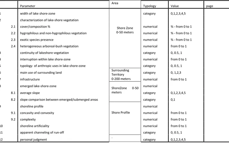
Table 6 shows for each parameter and subparameter, what is the area that the operator needs to consider, what is the typology (category or numerical) of the answer and its value range, and finally where to find more information on this manual. .
As previously described in chapter 3 (page 9 “the lake shore zone: ecology and function”), the lake shore zone is the transitional area that links the terrestrial environment to the pelagic one (Naiman & Decamps, 1997). For the purpose of this index, this consists of that “topographical strip situated around the lake that includes part of the littoral zone (up to a maximum depth of 1 m) and the strip of land that extends up to 50m from the shoreline”. The limit of 50 meters was set because literature reviews show how the buffer strip located between
Parameter Area Typology Value page
1 width of lake shore-zone category 0,1,2,3,4,5 2 characterization of lake-shore vegetation
2.1 cover/composition % numerical % - from 0 to 1 2.2 hygrophilous and non-hygrophilous vegetation numerical % - from 0 to 1 2.3 exotic species presence numerical % - from 0 to 1 2.4 heterogeneous arboreal-bush vegetation numerical from 0 to 1 3 continuity of lakeshore vegetation category 0, 0.5, 1 4 interruption within lake shore-zone numerical from 0 to 1 5 typology of anthropic uses in lake-shore-zone
Shore Zone 0-50 meters
category 0, 0.5, 1 6 main use of surrounding land category 0, 1,2,3 7 infrastructure
Surrounding Territory
0-200 meters numerical from 0 to 1
8 emerged lake-shore-zone numerical
8.1 average slope category 0,1,2,3,4,5 8.2 slope comparison between emerged/submerged areas
ShoreZone 0-50 meters
category 0,1
9 shoreline profile numerical
9.1 concavity and convexity numerical from 0 to 1
9.2 complexity numerical from 0 to 1
10 shoreline artificiality numerical from 0 to 1 11 apparent channeling of run-off
Shore Profile
category 0, 0.5, 1 12 personal judgment . category 0,1,2,3,4,5
Wet reeds and submerged hygrophilous species (see an open list on page 41, chapeter 6.2.2, table 7) are considered part of the lake shore zone. In this case, the 50 meters strip will move landward from the external limit of the reeds or of the vertical projection to the ground of the canopy of the hygrophilous species. In the case of lakes with reeds extending hundreds of meters lakeward from the shoreline (i.e Neusiedl lake, Austria), the full extend of the reeds can be included in the lake shorezone as it all has an ecotone function. Therefore, in this case, the lake shore zone will extend more than 50 meters from its lakeward limit.
In the case of an impermeable wall built along the shoreline, the lake shorezone width will be zero, as the wall prevents any buffer function.
Permeable walls that allow permeability do not represent a limit for the lake shore zone.
Artificial beaches, fertilized English garden are considered artificial structures just like the impermeable wall, but to differenciate them from cemented walls, they will be evaluated with a width from 0-5 meters.
When answering the questions (6 and 7) about the surrounding territory, the area that needs to be considered goes from the shoreline (thus, this does NOT include reeds or other hygrophilous species) to 200 meters inland. These questions are meant to evaluate the amount of human presence and the use of the territory. To answer these questions areal/satellite maps of the surrounding territory are very useful. (do not forget to add a scale bar when preparing the maps!).
The questions about the shore profile (9 to 11) regard the general shape of the external identified limit of the lake shore zone in the identified homogeneous stretch. Reeds may therefore increase the level of complexity of the shore (in the case of absence of impermeable walls).
The shoreline artificiality refers to a visual estimation of the level of anthropic influence along the shore, while to answer the questions about the apparent channeling run-off it is useful to have maps with countour lines to identify areas of fluxes concentration.
6.1 Width of the lake-shore-zone
1. width of lake shore-zone
0 0 1-5m 1 5-10m 2 10-30m 3 30-50m 4 >50m 5
Objectives of the question
The goal is to evaluate the cumulative width (in a orthogonal direction with respect to the water body) of all those formations (such as helophytes, hydrophytes, riparian and autochthonous shrubs, trees) able to carry a buffer function.
Principles
The efficency of the vegetation located in the shore zone is not only related to the complexity and diversity of the formations present, but also to its width. A shorezone width smaller than 30 meters, even when formed by trees and shrubs, can not efficiently carry out its function. The typology of vegetation cover also affects the level of functionality, therefore when estimating the width of the lake shorezone it is important to exclude that component that lack any buffer function.
What to look
First of all, it is necessary to identify unequivocally the lake-shore-zone. As already defined in Chapter 3, it corresponds to the zone that extends from the lake shores (the contact line between the aquatic and the terrestrial environment up to 1 meters water depth) landwards for a maximum length of 50 m. It includes functional vegetation formation in both the riparian and the littoral zones (Fig. 1). It can continue in forests and woods in the surrounding territory (to a maximum extend of 50 meters) or end earlier in the presence of an interruption. Interruptions are those structures of formation that limit the buffering power of the riparian zone. Examples are: roads, dirt roads that interrupt the vertical projection of the vegetation canopy, managed field, infrastructures, etc
An impermeable wall on the shoreline is considered as an interruption since it, reducing the width of the lake shorezone to zero.
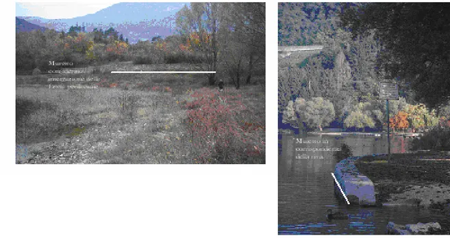
In the case of artificial or natural basins that are characterized by considerable and periodic changes in water level (causing the emergence of wide littoral areas), the shoreline considered should be the one of the maximum water level, recognizable by the separation between the temporarily submerged part and that portion colonized by stable vegetation.
The presence of wet reeds is to be considered within the lakeshore zone (only in the absence of impermeable walls on the shoreline). The internal limit towards the lake corresponds to the portion of the lake up to a depth of 1 m (Fig. 5). Within this zone there can be found both helophytes and hydrophytes.
Fig. 5 - Internal border of the lakeshores zone in the absence (yellow line) or in the presence (red line) of wet reeds.
Helophyte are semi-aquatic plants with the base and perennial buds submerged and with stem and leaves in the air; they are usually present on the lake and river banks, swamps and marshes where reeds are. Common examples are Typha (Typha latifolia, Typha longifolia), the Carex (Carex riparia, Carex flacca) and the marsh reed (Phragmites australis), the marsh reed (Schoenoplectus lacustris) the marsh Rumex (Rumex hydrolapathum), the water lily (Iris pseudacorus) and rice (Oryza sativa).
Hydrophytes are perennial aquatic plants whose buds are either submerged or floating; they are divided into rooted, with a root system attached to the bottom (e.g. Potamogeton spp, Nymphaea alba, Callitriche spp., Ranunculus spp., etc) and floating that do not have anchoring roots and float on the water surface (e.g. Lemna spp., Utricularia spp., etc.).
The width of the lake shore zone (trees, shrubs, wet or dry reed, etc.) is estimated in meters as a projection, on the horizontal plane, of the vegetation canopy. In the case of cliffs on the lake, it is considered lake shore zone only that portion next to the lake, excluding the rocky walls. If the lake shore zone is herbaceous, its width is evaluated only if it is represented by spontaneous formations, while mowed meadows or urban parks are excluded. In the presence of artificial beaches with mowed gardens, the width of the lake shore zone will be noticeably decreased. It could happen that the lakeshore zone has large trees, even scarce, under which there is a non-hygrophilous herbaceous growth; in this case, only the arboreal vegetation is considered while the herbaceous cover is not considered in the evaluation of the width.
How to answer:
Based on the width of the zone the following values are assigned:
0) the width of the functional formations is below a meter or inexistent or with only bare soil (little pebbles or sand). The answer is 0 (zero) also in the presence of infrastructures, impermeable walls or soil impermeabilization that reach the shore in the absence of reeds;
1) the width of the functional formations is between 1-5m; 2) the width of the functional formations is between 5-10m; 3) the with of the functional formation is between 10-30m; 4) the width of the functional formations is between 30-50m; 5) the width of the functional formations is more than 50m.
For survey purposes, the presence of impermeable walls, which is thus able to obviously affect the transverse continuum, is a limiting factor for the width of the lake shore zone vegetation (Fig. 6).
Whenever there is a band of well consolidated hygrophilous vegetation behind the permeable wall along the coast line (e.g. strip of willows and alder), the wall is considered only as an interruption (see page 6.4) and the vegetation is evaluated on its cover and composition.
Consequently, in the case of permeable walls or of other artificial structures that guarantee the permeability and the transversal continuity with the
surrounding territory, the vegetation present landward from the wall is considered as lakeshore zone vegetation.
Fig. 6: two examples of walls that represent an interruption of the lake shore zone. In the first case (above) the wall is not directly adjacent with the lake shore, while in the second case (right), the wall is right on the shore profile.
6.2 Characterization of the lake shorezone vegetation Objectives of the question
The following 3 parameters (composition/cover of the vegetation, percentage presence of hygrophilous and non-hygrophylous vegetation, presence of exotic species) are meant to describe the structure and composition of the lake shorezone.
Principles
The functionality of the lake shorezone depends on both its width and its composition/structure. Presence of grasses or bare soil will decrease the buffer functionality of the shorezone, while reeds and shrubs have higher filtering capabilities. Similarly, hygrophilous species indicate the presence of a riparian zone, which improved the buffering capability of the shorezone, while presence of exotic species is penalized.
6.2.1 Composition/cover
What to look
The composition of the vegetation of the lake shorezone is expressed in terms of cover with respect to the surface occupied by the zone itself (percentage value, then transformed into number from 0 to 1) of the vegetation categories showed in the table:
2.1 cover/composition % (expressed from 0-1)
trees % shrubs% reeds% grasses% bare soil% How to answer
In a homogenous stretch there could be meadows or beaches, reeds areas and/or tree areas: in this case each category will be analyzed and given a percentage. For example, if there is a zone composed of 75% “reeds” and 25% “arboreal species”, the values assigned will be 0.75 for the first and 0.25 for the second. The sum of the value given to the single categories will sum to 1, with the exception of the shore artificialization that will result with a total of 0 (as later described). Categories that are not present for at least 5% (value of 0,05) of the lake shore zone, will be given a value of 0 (zero).
The attribution of the percentages must start from the estimate of the portion of trees and shrubs, followed by the other categories beyond the projection of their canopy. Grass beneath the vertical projection of the tree canopy will not be considered. Therefore, in the case of large trees above a bed of grass, the “arboreal” and “shrubs” cover percentages will first be evaluated, and the remaining percentage value will the attribuites to “grass” and/or “bare soil”). In alpine and pre-alping lakes, if the lake shorezone is a natural environment that continues in the surrounding woodlands and forests, only the first 50 meters inland from the lake shores must be considered. If the identified lakeshore zone has an extension less than 50m, when limited by anthropic uses (i.e a road), the composition/cover percentage must be calculated only until the anthropic interruption.
In lowland, endoheic lakes, where the surrounding territory is mainly flat, the areas to be considered will correspond with the identified shore zone that has an ecotone function.
Whenever the lake shorezone is simply composed of a garden, the stretch will be given only a percentage in the category of “grass” (grass=1); in the case of a sandy or gravelly beach, the stretch will have a value of “bare soil” equal to 1. Artificial, fertilized gardens, like the ones found in cured touristic beaches or English gardens, will fall into the “bare soil” categories.
In the absence of vegetation in the lake shore zone, the answer of 1 will be given to the “bare soil” category, and 0 to all the others; in the case of infrastructure (e.g. wall, impermeable walls and embankments) or soil impermeabilization (e.g. harbour, parking area) on all the shore stretch, the value of 0 (zero) is given to all the categories.
Impermeable soils within the lake shore zone, such as cemented tennis courts, pools, housing or other, are considered in the “bare soil” category.
All the helophytes, such as Carex species, Sparganium species and Phragmites species, fall in the “reeds” category.
The hydrophytes with roots, submerged or with floating leaves and flowers possible present in the portion of the lake adjacent to the shore, as for example lilies (Nymphaea alba), yellow pond lilly (Nuphar lutea) and water chestnut (Trapa natans), are not considered into the lake shore zone and will therefore not be taken into account when filling the SFI form.
PLEASE NOTE: The “grass” category is important for the classification tree as it defines the route after the second node (see figure 4). In fact, for a “grass” value equal or less than 0.15 (15%), the route in the tree will go to the left, while values above 0.2 (20%) will lead to the right of the classification tree, with obvious differences in the resulting final evaluation (see Classification Tree, Figure 3).
For these reasons, in the case of a shore zone with a grass coverage borderline between 15-20%, the technician needs to evaluate carefully which percentage to attribute, as this component will result in route changes in the classification tree and thus in the final evaluation of functionality. The best approach is to identify the 20% limit (or 1/5 of the stretches surface free from the protection of tree-cover) and to decide whether the “grass” portion is superior or inferior to this limit and thus indicate it with a value of >0.20 (20%) if superior, and <0.15 (15%) if inferior.
6.2.2 Hygrophilous and non-hygrophilous vegetation
What to look
The presence of hygrophilous versus non-hygrophilous vegetation is estimated in this question and estimated in a percentage value (transformed in number from 0 to 1 as for question 6.2.1, the sum must be equal to 1).
How to answer
The category “hygrophilous vegetation” includes the helophytes, the shrub and arboreal species that are strictly riparian. An incomplete list of these is given in Table 7.
Whenever the whole stretch consist of “bare soil”, a value of 1 will be given in the “not hygrophilous” category. The same value is given in the presence of impermeabilization of the soil (blockage of water flows) throughout the entire stretch and in the case of impermeable walls which do not have any hygrophilous species behind it; in the case of a permeable wall or in presence of hygrophilous species, an intermediate value will be given as the wall only represent an interruption (see page with 6.1).
HYGROPHILOUS SPECIES family Common name
Alnus glutinosa Gaertn. Betulaceae Common alder
Carpinus betulus L. Corylaceae European or common hornbeam
Cornus sanguinea L. Cornaceae bloodtwig dogwood
Euonymus europaeus L. Celastraceae European spindletree Frangula alnus Mill.
(=Rhamnus frangula L.)
Rhamnaceae glossy buckthorn
Fraxinus excelsior L. Oleaceae Ash; also European Ash or Common Ash
2.2 Hygrophilous and non-hygrophilous vegetation (expressed from 0-1)
hygrophilous (helophytes, riparian shrub and riparian arboreal species) non-hygrophilous (other species)
Fraxinus oxycarpa Bieb. Oleaceae Raywood ash
Populus alba L. Salicaceae White poplar
Populus canescens (Aiton) Sm.
(=P. albo-tremula Auct.)
Salicaceae Gray poplar
Populus nigra L. Salicaceae Black poplar Prunus padus L.
(=Cerasus padus DC.=Prunus racemosa L.)
Rosaceae European bird cherry
Quercus robur L. (=Quercus peduncolata Ehrh.)
Fagaceae English Oak, Truffle Oak, Pedunculate Oak
Salix apennina A. Skortsov
(=Salix nigricans Sm. var. apennina Borzi)
Salicaceae Arctic willow
Salix cinerea L. Salicaceae Grey Willow; also occasionally Grey Sallow
Sambucus nigra L. Caprifoliaceae Elder or Elderberry Ulmus laevis Pallas
(= U. effusa Willd.)
Ulmaceae European White Elm, Fluttering Elm, Spreading Elm and, in the USA, Russian Elm
Ulmus minor Miller
(= U. campestris Auct. non L.; U. carpinifolia Suckow)
Ulmaceae Field Elm
Viburnum opulus L. Caprifoliaceae Guelder Rose, Water Elder, European Cranberrybush, Cramp Bark, Snowball Tree Tab. 6 - List of some hygrophilous species that characterize riparian environments of
lakes. Please note that this is an open list.
6.2.3 Presence of exotic species
What to look
In riparian environments there could also be exotic arboreal, shrub and herbaceous species. By “exotic” it is meant those species that are not-native, invasive or alien. The percentage of presence is recorded for this question.
Table 8 is an open list of the most common exotic species found in alpine and pre-alpine environments. (Table 7).
EXOTIC SPECIES family Common name
Robinia pseudoacacia L. Fabaceae Black locust
Ailanthus altissima (Miller) Swingle
Simaroubaceae Tree of Heaven
A R B O R E A L
Prunus serotina Ehrh. Rosaceae Black cherry
Buddleja davidii Franchet Scrophulariaceae Orange eye
butterflybush
Amorpha fruticosa L Fabaceae Desert false indigo
S H R U B S
Acer negundo L. Aceraceae Boxelder, Maple,
Maple Ash
Reynoutria japonica Houtt. Polygonaceae
Phytolacca americana L. Phytolaccaceae American Pokeweed
Sycios angulata L. Cucurbitaceae Single seeded
cucumber
Humulus scadens (Lour.)
Merril
Moraceae Japanese hop
Solidago gigantea Aiton Compositae Late goldenrod, great
goldenrod
Amaranthus retroflexus L. Amaranthaceae Redroot amaranth, redroot
pigweed, red rooted pigweed, common amaranth, common tumble weed
Ambrosia artemisiifolia L. Compositae Annual ragweed
2.3 Presence of exotic species (expressed from 0-1)