Landscape ecology and genetics of the wolf in Italy

A

Al

lm

m

a

a

M

M

at

a

te

er

r

S

St

tu

ud

di

io

or

ru

um

m

–

–

U

U

ni

n

iv

ve

er

rs

si

it

tà

à

d

di

i

B

B

o

o

lo

l

og

gn

na

a

DOTTORATO DI RICERCA IN

Biodiversità ed Evoluzione

Ciclo XXVI

Settore Concorsuale di afferenza: 05/I1

Settore Scientifico disciplinare: BIO/18

Landscape ecology and genetics of the wolf in Italy

Presentata da: Pietro Milanesi

Coordinatore Dottorato

Relatore

Prof.ssa Barbara Mantovani

Prof. Ettore Randi

Dott. Romolo Caniglia

1

2

The Wolves - Franz Marc, 1913

“ And when, on the still cold nights, he pointed his nose at a star and

howled long and wolf-like, it was his ancestors, dead and dust,

pointing nose at star and howling down through the centuries

and through him.”

3

I

NDEX

I

NTRODUCTION

4

M

ATERIALS AND

M

ETHODS

14

R

ESULTS

36

D

ISCUSSION

83

C

ONCLUSION

97

R

EFERENCES

100

4

I

NTRODUCTION

Large carnivores are often used as focal species (indicator species, umbrella species) in conservation strategies, especially when related to the maintenance of biodiversity. In fact, the conservation of populations of large predators is achieved through the conservation of their habitat and populations of their wild prey, influencing positively on the overall biodiversity. In addition, predators require natural habitats, extensive and continuous or strongly connected to each other, thus focusing attention on the importance of ecological corridors which benefit many other species (Huber et al. 2002). Large carnivores have also a key role with regard to the regulation of the populations of their prey: the wolf (Canis lupus), the lynx (Lynx lynx) and the bear (Ursus arctos) preferentially prey animals young and inexperienced or old and sick, helping to control the growth rates of the species prey. The wolf and the bear also feed on carrion, carrying out an activity of 'clean health', and this helps to prevent the onset of diseases, improving the health of the animals (Breitenmoser 1998). Finally, the persecution of man towards predators requires effective legislation and strict enforcement, especially because the long period of absence of large carnivores in several regions of Italy has created many problems in the management of conflicts between the presence of the species and the husbandry activities of the resident human population. For these reasons, wolf, bear and lynx are protected both at international and national level: included in Annex II of the Bern Convention ("strictly protected fauna species"), attachment II ("Animal and plant species of Community interest whose conservation requires the designation of special areas of conservation") and 4 ("Animal and plant species that require strict protection") of the Habitats Directive, Annexes A and B of the Washington Convention (CITES) and Art. 2 of the Regulations 157/92 ("specially protected species"). The extraordinary ability to adapt to different ecological conditions made the wolf the terrestrial mammal predator with the largest distribution range during the Quaternary, covering, north of 20° N latitude, the entire North American continent, including Mexico, Europe, Asia and Japan (Mech 1970, 1974). However, in historical times, the massive eradication efforts carried out by humans since the 19th century, direct and indirect (reduction of natural habitat and wild prey by hunters), resulted in a drastic reduction in both distribution and abundance. During the 20th century the wolf also disappeared from almost all the territories of continental Europe, surviving in small and fragmented populations in the Iberian, Hellenic and Italian peninsula, in some territories of the former Yugoslavia and in the Scandinavian peninsula. Actually, the European wolf range interests the Iberian Peninsula, which has a population of 1,500-2,000 wolves (Blanco et al. 1990; Salvatori et al. 2005), the Balkan countries and the Hellenic

5

peninsula. In France, signs of recovery are in the Mercantour Massif in the Southern French Alps: right through the Maritime Alps the wolf is gradually colonizing the South-western areas of the Swiss Alps. To date, it is believed there are about 80 wolves in the French Alps, all from the Apennines (Salvatori et al. 2005). Also in the rest of Europe wolf populations are growing or stable and the low degree of human settlement of large areas of European Russia allows the maintenance of high numerical amounts and it is also responsible for the slow processes of expansion of the species toward the central-eastern countries such as Romania and Poland, where about 4,000 and 600-700 individuals are estimated respectively (Salvatori et al. 2005) confined to forest areas of mountain territories. In northern Europe wolf populations are divided between the Scandinavian peninsula, where it is estimated that about 200 people, and the Baltic States, whose wolves are from Russia (Salvatori et al. 2005).

Figure I.I Distribution of wolf in Europe (in orange; http://www.lcie.org/)

In Italy, the wolf widespread over the entire peninsula until the mid-19th century, was exterminated in the Alps at the end of that century and in Sicily island in 1940. Just in the last century, the distribution of the species suffered a significant drop along the Apennine chain. At the end of the 50s it became very rare throughout the Tuscan-Emilian Apennines and in the following decade the large number of species decreased dramatically to reach a historic bottleneck in the early '70s, when Zimen and Boitani (1975) estimated the presence of about 100 wolves in the Southern-Central

6

Apennine. Since that time, there was a gradual and continuous expansion of the territories occupied by permanent wolf favoured by several factors: socio-historical, such as the abandonment of mountains and hills by the local human populations resulting in an increase of forested areas and uncultivated fields, the creation of protected areas and the implementation of conservationist policies (Bocedi and Brcchi 2004), the reintroduction of wild ungulates and the numerical reduction in the number of hunters and also biological characteristics of the species (dispersal ability and trophic opportunism). The re-colonization of the historical range is still on-going. The current distribution of the wolf in Italy includes the entire Apennine chain, from Liguria to Calabria, the hilly areas of Northern Lazio and central-Southern Tuscany and the and Maritime Alps, from which the predator is re-colonizing the Alpine chain. Wolf packs are stable in all the mountainous provinces of Piedmont and Valle d'Aosta, at the border with France and Switzerland, with an estimated population of more than 50 individuals in the two regions (Marucco 2010). Few individuals were recorded also in the central Alps (Lombardy, Trentino Alto Adige and Veneto) while individuals from Slovenian are re-colonizing the eastern alps (Friuli-Venezia-Giulia).

7

This quick reverse trend of the wolf has determined the need for long-term conservation actions, in fact viable wolf populations entails solving both biological and human-dimension problems (Ciucci et al. 2007; Linnell and Boitani 2012), because in the minds of the public a strong aversion to the predator remains, created through a negative cultural transmission, no longer mitigated by direct experience, resulting from the coexistence between humans and wolves in the same environment. Moreover, the absence of the large carnivore in the Alps and the Apennines meant that they were no longer taken the usual and tested methods of preventing damage to the animal husbandry and evolve towards more and more forms of breeding in wild, with poor control of animals bred, more economical and profitable. The wolf, like other large carnivores, to feed optimize the energy balance of costs and benefits, so it attacks prey with equal amount of energy supplied to require the least amount of energy. Thus, the most common prey animals are debilitated, sick, young, or animals for their behavioral characteristics (also induced) can be easily preyed upon. It is the case of domestic animals (goats, sheep, cows and horses) which, living in contact with humans and not having long experienced the attacks of predators, have lost, in part, the behavioral mechanisms of defense. Finally, the increase in the population of wild ungulates, which occurred in the last ten years, created a marked interest for hunting these species, which easily come into conflict with the presence of the wolf, a typical predators of large herbivores and, “consequently”, human hunter competitors. Beyond their actual predatory ability, and their real economic impact, carnivores are related to myths and legends that definitely not conducive to their preservation. The images of wolves who eat children and attacking travelers along the mountain trails are a historical legacy handed down from generation to generation, which now needs to be removed with appropriate information actions, based on scientific knowledge of the real behavior of predators in respect of the real impact on human activities. Thus, the wolf should still be considered as a threatened species, because of the conflicts with human activities that are triggered by its predatory behaviour and that lead to illegal persecution. This in turn makes the colonization of new areas unstable, in particular those where livestock husbandry is an important economic activity (Genovesi 2002).

In this Ph.D. thesis, to understand the real effect of wolf predations on prey species the diet of the large carnivore in Italy was analysed and then the changes of feeding habits of the species trough years, seasons and different areas were verified. Understanding the mechanisms that lead to changes of feeding habits and predatory impact of large carnivores is of great importance in outlining effective strategies for their conservation. One of the cruxes of the management of the conflicts between human activities and large predators lies in understanding if the extent predation is a regulatory or limiting factor acting on wild prey populations, and how it is possible to reduce the impact on domestic livestock. Regarding the relationships between wolves and wild ungulates, the

8

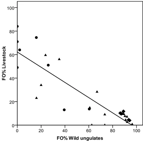
main question is whether predation can regulate the populations of these prey species. Usually in a prey-predator system regulation occurs when predation is density dependent and it stabilizes prey populations at an equilibrium density. However, if predation is independent on density there is a limiting effect and if it is inversely density dependent there is a dispensatory effect. In these cases predation rate increases as prey density declines, causing the population to decline even faster; this situation can occur when there is no switching by predators, there is no refuge for the prey, and predators have an alternative prey source (Messier 1991, 1995; Marshal and Boutin 1999; Jedrzejewski et al. 2002; Wittmer et al. 2005; Sinclair et al. 2006). In simple wolf-prey systems wolf diet shifts according to changes in the relative abundance of the main prey, and shift dynamics depend on the combined effects of preference, differential vulnerability and the relative abundance of prey (Peterson and Ciucci 2003; Garrot et al. 2007). In areas with rich and abundant wild ungulate guilds wolves prey upon the most abundant and profitable species, selecting gregarious ones, young, and those in poor physical condition, and changing their preferences in relation to species abundance (Okarma 1991; Huggard 1993a,b; Mattioli et al. 1995; Okarma 1995; Meriggi et al. 1996; Poulle et al. 1997; Jedrzejewski et al. 2000; Mattioli et al. 2004; Gazzola et al. 2005, Ansorge et al. 2006; Gazzola et al. 2007; Barja 2009). In areas with low wild ungulate abundance livestock is the main prey and wild ungulates occur in wolf diet when livestock is not available or when young wild ungulates are present (Cuesta et al. 1991; Meriggi et al. 1991, 1996; Okarma 1995; Meriggi and Lovari 1996; Vos 2000; Hovens and Tungalaktuja 2005). Moreover, predation by wolves on livestock is dependent on the species, age class, rearing methods, and on the availability of wild prey (Robel et al. 1981; Blanco et al. 1990; Meriggi et al. 1991; Boitani and Ciucci 1993; Meriggi and Lovari 1996; Kaczensky 1999; Mech et al. 2000; Bradley and Pletscher 2005; Gazzola et al. 2008). In particular wolves select sheep and goats, and from cattle calves less than 15 day old (Meriggi et al. 1991, 1996; Gazzola et al. 2008). High occurrence of livestock in wolf diet was also recorded in areas of year-round grazing or where livestock is grazing unguarded (Meriggi et al. 1996, Merkle et al. 2009) and damage is concentrated to a few farms, suggesting that environment is also important in determining the probability of predation (Kaczensky 1999; Schenone et al. 2004; Bradley and Pletscher 2005; Gazzola et al. 2008). From an analysis of the diet of wolves in Mediterranean ranges, a close negative correlation was observed between the frequency of occurrence of livestock and that of wild ungulates; this may mean that wolves prefer wild prey, when available, to domestic ones (Meriggi and Lovari 1996). Where the availability of wild ungulates is low and livestock is absent or inaccessible wolves use secondary prey species that can be necessary dietary components in some seasons (Van Ballenberghe et al. 1975, Fritts and Mech 1981, Fuller 1989, Chavez and Gese 2005). Moreover, several studies have shown some

9

important differences between wolf feeding habits in different study areas and periods. Wolf feeding habits can also change over different periods within the same area, usually as a response to the increase of wild ungulate populations. In Mediterranean countries in particular, a positive trend of wild ungulate occurrence in wolf diet has been recorded in recent decades (Meriggi and Lovari 1996), and this is true also for recently settled wolf populations in Central Europe, where it seems that the current diet is very different from that before wolf extinction (Ansorge et al. 2006). In fact, also in Italy the diet of wolves markedly changed from the first studies carried out in the seventies in the central Apennines to the recent ones performed in the Western Alps; in particular the diet of wolves evolved towards a greater occurrence of large wild herbivores, becoming more and more similar to that of North American and North-Eastern European areas (Meriggi and Lovari 1996). Changes in the diet of wolves in Italy were identified and related to the use of wild ungulate species, to the differences in large prey availability and to the richness and diversity of wild ungulate communities. Moreover, the patterns of prey selection and their seasonal changes were evaluated.

In this Ph.D. thesis, secondly, the distribution and population dynamics of wolves in the northern Apennine was estimated using noninvasive genetic methods, because the expanding population also spread in human-dominated areas, where the chances of hybridization with domestic dogs may increase (Verardi et al. 2006; Godinho et al. 2011; Hindrikson et al. 2012; vonHoldt et al. 2013) and the attribution of species locations could lead to mistaken estimates. The development of noninvasive genetic methods has offered unique opportunities to implement long-term, wide-ranging, and cost-effective research and monitoring programs (Schwartz et al. 2007; Brøseth et al. 2010; Ruiz-Gonzalez et al. 2013). Molecular techniques can provide more-exhaustive demographic information than any other method (Lukacs et al. 2007). Reliable individual genotypes (DNA fingerprinting) are obtained by analyzing DNA extracted from biological samples such as hair, feces, urine, and blood traces that are noninvasively collected, without any direct human contact with the animals (Waits and Paetkau 2005). Genotypes are used to count and locate individuals in space and time and to reconstruct their genealogies and familial ranges (Creel et al. 2003; Schwartz et al. 2007). The capture–recapture records of individual genotypes can be used to count the minimum population size (Ernest et al. 2000; Lucchini et al. 2002; Gervasi et al. 2008) and to estimate total abundance (Kohn et al. 1999; Mills et al. 2000; Lukacs and Burnham 2005). Although low-quality DNA samples may generate genotyping errors (Broquet et al. 2007), these can be minimized by using well-tested laboratory protocols and quality controls (Beja-Pereira et al. 2009). Noninvasive genetics has been used to monitor the dynamics of endangered populations, obtaining estimates of temporal trends of demographic and genetic parameters that would have been

10

impossible with traditional field methods (e.g., De Barba et al. 2010). The reconstruction of pedigrees in natural populations (Pemberton 2008) is facilitated by genetic identifications, which substantially help to infer detailed population structuring, and to estimate dispersal rates, inbreeding, and heritability (vonHoldt et al. 2008), pushing the development of novel computational methods (Blouin 2003). For these reasons, noninvasive genetic sampling has been integrated into many monitoring projects, combining population genetics and demographic data in species of large carnivores (Waits and Paetkau 2005), including studies of wolves (Fabbri et al. 2007; vonHoldt et al. 2008; Marucco et al. 2009; Cubaynes et al. 2010; Stenglein et al. 2011). Most wolves are territorial, social carnivores that live in packs, the basal family units, which generally include a breeding pair, the offspring from several years, and sometimes unrelated wolves (Mech 1999). Packs scent mark and defend their territories, and territories often remain stable for several successive breeding pairs. Pack members cooperate in hunting and rearing pups (Mech and Boitani 2003). Pack size and composition, prey abundance, and habitat availability determine the demographic trends of wolf populations (Fuller et al. 2003; Stahler et al. 2013). In turn, variable mating behaviors, turnover rates of pack breeders, dispersal patterns, and inter-pack gene flow affect population genetic structure and long-term evolutionary dynamics (Lehman et al. 1992; Lucchini et al. 2004; vonHoldt et al. 2008; Sastre et al. 2011; Czarnomska et al. 2013). In this way, pack dynamics, natural selection, adaptation, and inbreeding avoidance affect kin structure and inbreeding and determine the evolution of genetic variability (Keller and Waller 2002; Bensch et al. 2006; Coulson et al. 2011; Geffen et al. 2011). Determining wolf population structure and dynamics, however, is not trivial (Duchamp et al. 2012). Wolves are distributed at low densities across large geographic areas, often in forested mountain regions, and their individual and familial home ranges are wide (Jedrzejewski et al. 2007). In these conditions, standard field methods based on direct observations, livetrapping and radiotelemetry, snow-tracking, and distance sampling (Wilson and Delahay 2001; Meijer et al. 2008; Blanco and Cortes 2012) are challenging or exceedingly expensive at a large scale (Boitani et al. 2012; Galaverni et al. 2012). Consequently, most of the published studies report details based on short-term, empirical studies (i.e., Scandura et al. 2011). The result is that values of crucial demographic parameters such as survival, abundance, turnover, dispersal, and reproduction rates remain poorly known (Mech and Boitani 2003). Here, the results of a 9-year noninvasive genetic monitoring in a wolf population that recently recolonized the Apennine Mountains of the Northern Italy were summarized (Caniglia et al. 2010, 2012). This research was designed also to determine the genetic variability and integrity of the population, which might have been threatened by reduced effective size and hybridization with domestic dogs (Randi 2011); the number of packs (Mech and Boitani 2003); the size of the packs, including the

11

number of unrelated (adoptee) wolves (Jedrzejewski et al. 2005); the relatedness of individuals in the packs and the frequency of inbred reproductive pairs (Lehman et al. 1992; vonHoldt et al. 2008); and the frequency of pack splitting during the process of population expansion (Jedrzejewski et al. 2005). Based on the territorial and hierarchical organization of wolf populations (Mech 1999), locations and composition of the wolf packs predicting that dominant individuals would be sampled within defined geographic ranges were reconstructed (corresponding to their territories - Fuller et al. 2003); distinct packs would have non-overlapping ranges, thus dominants from distinct packs would be sampled in non-overlapping areas (Apollonio et al. 2004; Kusak et al. 2005, vonHoldt et al. 2008); dominants would mark their territories with scats and urine (Zub et al. 2003; Barja et al. 2005), so they would be sampled more frequently than young or transient individuals; breeding pairs should reproduce for at least 1 breeding season, and consequently would be sampled longer than young or transients (Mech and Boitani 2003); and pedigrees of familial groups could be reconstructed, given the power of the molecular markers used for genotyping (Pemberton 2008). The results clarify details of wolf social behavior and wolf population dynamics in an area with diverse habitats and prey availability, and provide the basis necessary to forecast future demographic trends and ecological roles of wolves in Northern Italy.

Large carnivores represent also a special case in which the identification of species and individuals is fundamental for the attribution of depredation on livestock (Caniglia et al. 2013) and thus, the third aim of this thesis was to identify the main factors influencing the wolf distribution and provide depredation risk maps as a tool for managers and shepherds to prevent predator attacks. However, the identification of the predator and its presence in an area are not sufficient to predict where an attack could occur. Modeling habitat-species and predator-prey relationships in human-dominated landscapes could play an important role to design large carnivore conservation strategies, especially to reduce conflicts with human activities (Treves et al. 2004). The method consisted in the identification of the pastures with the highest risk of predation, based on a long-term molecular research on wolves. To identify the areas where the presence of the wolf could lead to predation on livestock, season-specific models were formulated, because wolf habitat selection changes from the grazing (GP; April-September) to the non-grazing (NGP; October-March) period as a consequence of variation in resource availability (Milanesi et al. 2012). Ecological niche modeling provide a suitable way to analyze presence-only data, as they compare the values of environmental variables in the entire study area (the availability distributions), to those in locations where the species has been sampled (the utilization distributions; Calenge and Basille 2008). Thus, the General Niche Environment System Factor Analysis (GNESFA; Calenge and Basille 2008) was computed with wolf genotypes identified during a 12-year monitoring project in a study area of 71,443 km2 in

12

North-Central Apennines and South-Western Alps (Italy) and then, the resulting GP habitat suitability maps was used to define depredation risks on livestock in pastures (Kaartinen et al. 2009; Marucco and McIntire 2010). Even if wolves are protected by law in Italy and in most of the other European countries, its predatory behavior could lead to heavy poaching, which is estimated to kill c. 20% of the population each year in Italy (Lovari et al. 2007, Caniglia et al. 2010) and then, conservation strategies, aimed at reducing conflicts with human presence and activities, should be designed based on accurate population monitoring and predation risk assessment (Treves et al. 2004). The genetic analyses of all the collected presumed wolf scat samples, necessary for the analyses, were performed at the Genetic Laboratory of the Istituto Superiore per la Protezione e la Ricerca Ambientale (ISPRA).

By combining landscape ecology and population genetics aspects, in this thesis, finally landscape genetics patterns of the wolf population in Italy were investigated. Landscape genetics assesses how the environment affects the movement, dispersal or gene flow of species (Segelbacher et al. 2010) and thus gives evidence of functional connectivity within landscapes (Holderegger et al. 2007; Holderegger and Wagner 2008). Landscape genetics often uses least cost path (LCP; Cushman 2006) analysis from resistance surfaces to movement to measure ecological distances among populations or individuals. These ecological distances are then correlated to genetic distances. In LCP analysis, different levels of resistances to movement must be assigned to particular landscape elements. These resistance values are mostly based on expert opinion (Clark et al. 2008; Lee-Yaw et al. 2009; Murray et al. 2009) and have usually not been evaluated from empirical data such as direct observations, dispersal behavior or GPS and radio-tracking (Stevens et al. 2006; Epps et al. 2007; Chietkiewicz and Boyce 2009). However, expert knowledge can lead to subjective uncertainty and strongly influence the results of landscape genetic analysis (Cushman et al. 2010; Cushman and Lewis 2010; Huck et al. 2010). Alternatively, habitat suitability models, based on distribution data of species, could be applied as a potentially more objective means to assign resistance values in LCP. Here, the reciprocal of the value of a habitat suitability model is directly used as a values for the resistance to movement of particular landscape elements (Wang et al. 2008). Expert knowledge is therefore not involved in the assignment of resistance values. The use of habitat suitability models in landscape genetics is, however, not without caveats. First, there is often bias in the locations of samples or observations, used for modeling habitat suitability, and species might also have different detectability in different landscape elements (O’Brien et al. 2006). Second, Spear et al. (2010) highlighted that suitability models mainly reflect the reproductive habitat or the home range of species but not necessarily movement through the landscape during dispersal. Habitat suitability models might therefore ignore critical features of inter-population

13

movement and dispersal. Nevertheless, Laiola and Tella (2006) and Wang et al. (2008) presented two empirical applications of habitat suitability models in landscape genetics, which showed significant correlations between genetic distances and resistance surfaces based on habitat suitability. Similarly, Brown and Knowles (2012), Duckett et al. (2013) and Wang et al. (2013) successfully used different types of habitat suitability models in landscape genetics. A large variety of habitat suitability models have been developed during the recent years, and comparisons of different methods were carried out to find the best model to define species distributions or to forecast population expansions (Jones-Farrand et al. 2011). However, most of the landscape genetic studies that applied habitat suitability modeling used only one particular habitat suitability model in their analyses. Hitherto, no thorough comparison and evaluation of different habitat suitability models, to assign resistance values in LCP modeling and landscape genetics, has been carried out. The aim was to find habitat suitability models that provided highest efficiency in LCP prediction and landscape genetic analysis. For this purpose, ten widely used habitat suitability models were

applied to identify suitable habitat and validated their efficiency. According to Wang et al. (2008) and Pullinger and Johnson (2010), resistance values were calculated from the resulting habitat suitability maps as 1 – habitat suitability. Ecological distances were determined as the length along LCPs as well as straight-line Euclidean (geographical) distances (Etherington and Holland 2013; Van Strien et al. 2012). Then, the power of the ecological distances obtained from the ten different habitat suitability models was evaluated to explain genetic distances while also considering the effects of Euclidean distance in a landscape genetic framework. Thus, partial Mantel tests, which are traditionally used in landscape genetics, multiple regression on distance matrices, which is the state of the art method of statistical analysis in landscape genetics, and fore-front mixed effect models were applied (Van Strien et al. 2012). The data set consisted of about 1,000 wolves originating from a long-term genetic monitoring program (12 years) across a large study area of about 100,000 km2 in Italy. The landscape genetics analyses were performed at the Research Units of Biodiversity and Conservation Biology if the WSL Swiss Federal Research Institute.

14

M

ATERIALS AND

M

ETHODS

M.1. Changes of wolf diet in Italy in relation to the increase of wild ungulate abundance

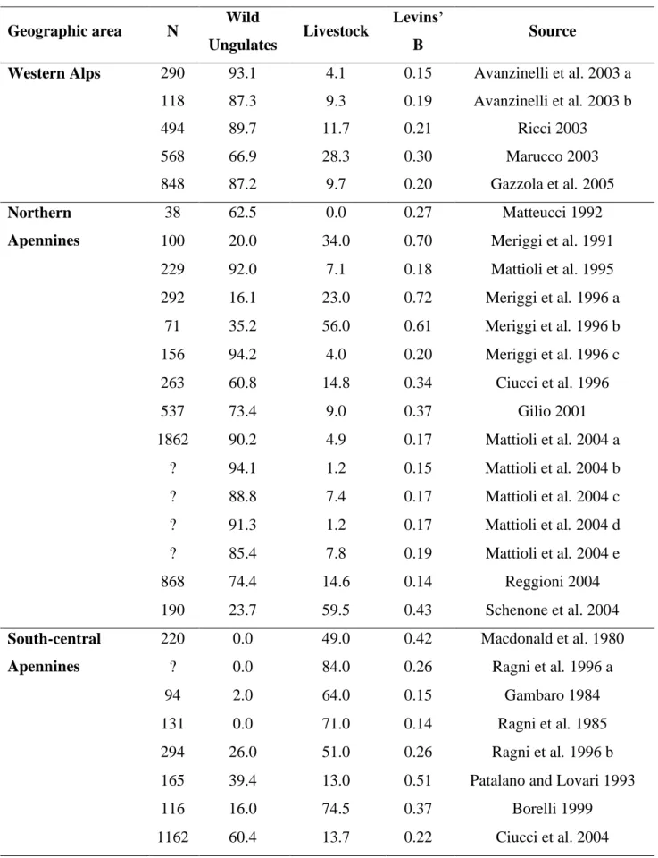
An analysis of the scientific papers about the feeding habits of wolves in Italy was carried out taking into consideration the studies on the analysis of scats because they were more numerous than those that used predation data. Studies published in scientific journals, degree, masters and PhD theses, and unpublished reports were considered. If a study summarized results from more than one study site, these were analyzed separately, i.e. per site.

For each study, the absolute percentage of occurrence (ratio between the number of times that a prey occurs in the sample and the sample size) of seven food categories (Wild ungulates, Livestock, Small mammals, Other vertebrates, Fruits, Other vegetables, Garbage) was considered and then the percentage of occurrence calculated for each wild ungulate species. Moreover, the diet breadth was calculated by the normalized Levins’ B index on food categories (Feisinger et al. 1981).

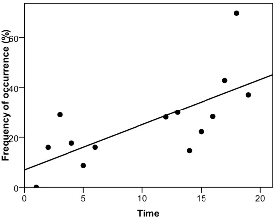
At a local level, the data on wolf diet from the Genova province (northern Apennines) from 1987 to 2005 was considered, computing for each year the frequency of occurrence of pooled wild ungulates, and of each species that occurred in scats.

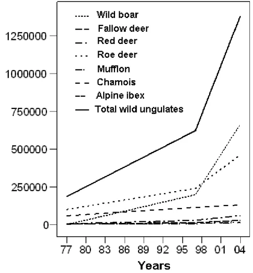
Population estimates of the different species of wild ungulates in Italy was extrapolated from Pavan and Berretta Boera (1981), Pedrotti et al. (2001), and Apollonio (2004); the trend at national level was obtained by extrapolation, assuming a constant numeric increase between time intervals (years), thus obtaining a rate of increase that linearly decreases with the increase in population. The diet composition of wolves among geographic areas was compared by nonparametric multivariate analysis of variance (NPMANOVA; Anderson, 2001; Hammer, 2010) with permutation (10,000 replicates) and pairwise comparisons with Bonferroni’s correction; furthermore, each variable was tested with the Kruskall–Wallis test. For this aim the examined studies were assigned to the following geographic areas: southern-central Apennines (Region administrations: Umbria, Abruzzo, Calabria), northern Apennines (Region administrations: Piedmont, Lombardy, Liguria, Emilia-Romagna, Tuscany), and western Alps (Region administration: Piedmont) (Fig. M.1.1).

To show significant trends of wild ungulate and livestock use and of diet breadth, curve-fit analyses were used with the time as independent variable. The same type of analysis was used to show the type of relationships between wild prey usage and their abundance.

15

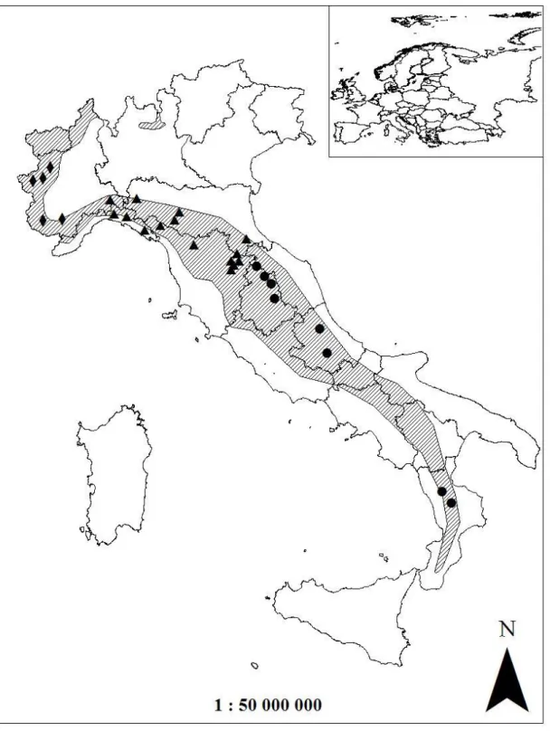
Figure M.1.1 Distribution of the analyzed studies on wolf diet in Italy carried out from 1976 to 2004 (circles: south-central Apennines; triangles: northern Apennines; diamonds: western Alps; shaded area: wolf range).

16

M.2. Selection of wild ungulates by wolves in an area of the Northern Apennines (North Italy)

Study area

in the study area covered an 860 km2 mountain area located in the western part of the Northern Apennines (North Italy: 44°46’17.40’’N, 9°23’11.04’’E) with elevations of 500-1700 m a.s.l.. The community of wild ungulates included, in order of abundance: wild boar (Sus scrofa), roe deer (Capreolus capreolus, fallow deer (Dama dama), and red deer (Cervus elaphus). The last two species were localized in two distinct parts of the study area, and the former two were widespread over the whole territory. Wild boars shot by hunters increased from 600 individuals in the nineties to 2650 in 2008, roe deer densities, estimated by drive and vantage point counts, increased from 5.9 per km2 in 2005 (the first year of census) to 8.6 per km2 in 2008, fallow deer density averaged 1.9 per km2 from 2006 to 2008 (drive and vantage point counts), and red deer roaring males increased from 22 in 2002 to 33 in 2008 (data from the Wildlife Services of the provinces of Piacenza and Pavia). Livestock was present on pastures located on the ridges of mountain chains from April to October; mainly cattle but also goats, sheep, and horses were free ranging during the grazing period. Their numbers were constant over the last twenty years: cattle amounted to 1996 heads, goats and sheep to 757, and horses to 157 (data from veterinary services of the provinces of Piacenza and Pavia).

By snow-tracking, wolf-howling and camera-trapping, a presence of four main packs of wolves was estimated in the study area, respectively of 7, 5, 4, and 2 individuals, and a small number of lone wolves. The presence of free ranging or feral dogs has never been recorded in the study area and the wolf was the only species of large carnivore present in this region.

Data collection

Itineraries traced on footpaths and randomly chosen (N=25) were selected among those existing in the study area (total length = 168 km, average ± SD = 7.0 ± 2.3 km, min. = 2.8 km, max. = 11.3 km). From June 2007 to May 2008 all transects were covered once a season (winter: December to February; spring: March to May; summer: June to August; autumn: September to November) searching for wolf scats and signs of wild ungulate presence. On itineraries, all fresh wolf scats were collected and wild ungulate signs were recorded (tracks, rooting, resting sites, wallowing, and rubbing), in order to estimate the proportions of use and availability of the different species.

17 Diet analysis

Wolf diet was studied by scat analysis. Scats were preserved in PVC bags at -20°C for one month, and then they were washed in water over 3 sieves with decreasing meshes (0.5-0.1 mm). Prey species were identified from undigested remains: hairs, bones, hoofs, and nails (medium and large sized mammals), hairs and mandibles (small mammals) seeds and leaves (fruits and plants). Moreover, hairs were washed in alcohol and identified by microscopical observation of cortical scales and medulla (Brunner and Coman 1974; Debrot et al. 1982; Teerink 1991; De Marinis and Asprea 2006).

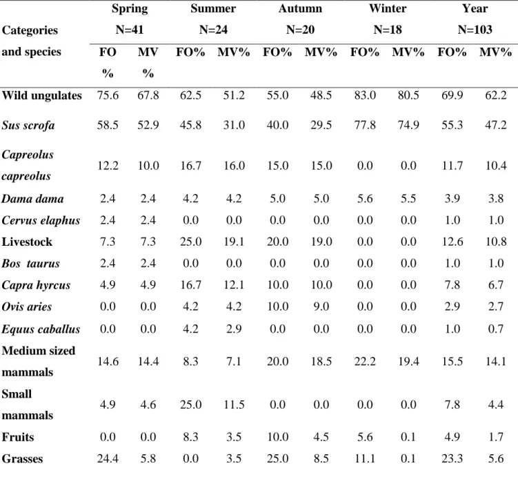
The proportion of prey was assessed for each scat as they were eaten (Kruuk and Parish 1981; Meriggi et al. 1991, 1996; Meriggi and Lovari 1996) and each prey was assigned to one of the following percent volumetric classes: <1%; 1-5%; 6-25%; 26-50%; 51-75%; 76-95%; >95%. All the identified preys were grouped into 5 food categories (Wild ungulates, Livestock, Medium sized mammals, Small mammals, and Vegetables). For each food category and species of wild and domestic ungulates was calculated: i) percent frequency of occurrence (FO%), and ii) mean percent volume considering all the examined scats (MV%). Moreover, for wild ungulate species, the relative consumed biomass (%) was calculated following the method proposed by Floyd et al. (1978) and using the regression equation formulated by Ciucci et al. (2001) on European prey species of wolves:

y = 0.274 + 0.011x

where y is the biomass (kg) of prey for each collectable scat and x is the live weight of prey. The average weight of wild boar and fallow deer was calculated from local data of shot individuals (59.4 kg and 56.5 kg respectively), while the average weight of roe deer and red deer were calculated from literature data (roe deer: 20.7 kg, Soffiantini et al. 2006; red deer: 98.5 kg, Mattioli and Nicoloso 2010).

Statistical analysis

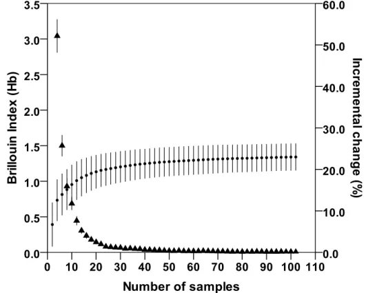
The adequacy of sample size was assessed using the method proposed by Hass (2009). Brillouin index (1956) was calculated:

where Hb is the diversity of prey in the sample, N is the total number of individual prey taxa in all

samples and ni is the number of individual prey taxa in the ith category. A diversity curve was then

calculated by increments of two samples randomly taken. For each sample, a value of Hb was

calculated and then re-sampled 1,000 times by the bootstrap method to obtain a mean and 95% Confidence Interval. Adequacy of sample size was determined by whether an asymptote was

18

reached in the diversity curve and in another curve calculated from the incremental change in each Hb with the addition of two more samples. Both curves were plotted against the number of analyzed

scats.

Seasonal variations of the frequency of occurrence of food categories and ungulate species were analysed by the Likelihood ratio test (exact test with permutation, 10,000 replicates). Seasonal differences of the mean percent volume of food categories and ungulate species were tested by Nonparametric Multivariate Analysis of Variance (NPMANOVA) with permutation (10,000 replicates) and pairwise comparisons using Bonferroni correction. Furthermore, each variable was tested by the Kruskall-Wallis test with permutation (10,000 replicates) and pairwise comparisons with adjusted P-values (Dunn 1964).

Wolf diet breadth was estimated in each season by the B Index (Feisinger et al. 1981):

Where pi is the proportion of usage of the ith prey item and R is the number of prey items found in

the diet. The index ranges from 1/R (usage of one item only) to 1 (when all items are equally used). To test for significant differences of the B index among seasons wolf scats were re-sampled 1,000 times by the bootstrap method and calculated the B index for each bootstrap sample, in order to estimate the average and the confidence interval at 95% of the index distribution (Dixon 1993; Hesterberg et al. 2005). Then, the superposition of confidence intervals between each pair of seasons was verified. Wolf selection of wild ungulate species was evaluated by the Manly preference index α (Manly et al. 2002):

Where OUPi is the observed usage proportion for the ith species calculated from the estimated

biomass, and EUPi is that expected on the basis of the species availability (i.e. the proportion of

presence signs detected on itineraries for each species). When preference does not occur, αi= 1/n,

for each i= 1,...,n. If αi is greater than 1/n, then the species i is selected. Conversely, if αi is less than

1/n, species i is avoided. To test the reliability of the Manly index, wolf scats were re-sampled 1,000 times by the bootstrap method. Then, the average values and the 95% confidence intervals of the Manly index was calculated in order to verify significant differences of the index values among wild ungulate species and among seasons, and from the value 1/n. Finally, the wolf diet resulting from the study with the wolf diet in the same area between 1988 and 1990 was compared. The comparison was carried out through the Likelihood ratio test with permutation (10,000 replicates) on frequency of occurrence of the food categories.

19

M.3. Noninvasive sampling and genetic variability, pack structure, and dynamics in an expanding wolf population

Sample collection

Noninvasive samples (mainly scats) were collected from March 2000 to June 2009 by more than 150 trained collaborators, including staff of the Italian State Forestry Corps, park rangers, wildlife managers, researchers, students, and volunteers. Although the external appearance of scats might not reflect their age (Santini et al. 2007), collectors were trained to collect samples as fresh looking as possible, excluding the most degraded ones. Feces were collected along a total of approximately 160 trails or country roads averaging about 6.1 km in length. Roads and trails were chosen opportunistically based on known or predicted wolf presence, as assessed by field surveys of wolf trails and snow tracks, documented kills, wolf-howling, or occasional direct observations, approximately covering the entire range of stable wolf distribution in the study area. Roads and trails were surveyed at least once per month, on average, either on foot or by car. Samples of muscle tissue were obtained from wolves killed accidentally or illegally. Blood samples were occasionally obtained during rescuing operations on wolves wounded or in poor health condition. Fecal sample collection did not require any direct interaction with the animals. The tissue samples were obtained from found-dead wolves legally collected by officers on behalf of the Italian Institute for Environmental Protection and Research (Istituto Superiore per la Protezione e la Ricerca Ambientale). No animal was sacrificed for the purposes of this study. Blood samples were obtained from rescued animals by appropriately trained veterinary personnel. Anesthesia was used whenever necessary to minimize any stress on the animals during handling procedures. All the procedures followed guidelines approved by the American Society of Mammalogists (Sikes et al. 2011). The coordinates of every sample (Fig. M.3.1) were recorded either on a 1:25,000 topographic map or by global positioning system devices, then digitalized on ARCGIS 10.0 (ESRI, Redlands, California). The large study area and long-term program did not allow us to standardize or randomize sampling in space and time. Nevertheless, as highlighted in Jedrzejewski et al. (2008), heterogeneity should not bias the results in any systematic way. Small external portions of scats and clean tissue fragments were individually stored at -20°C in 10 vials of 95% ethanol. Blood samples were stored at -20°C in 2 vials of a Trissodium dodecyl sulfate buffer. A total of 5,065 samples were collected including 4,998 scats, 4 hair tufts, 2 urine stains found during snow-tracking, 57 samples of muscle tissue obtained from wolves killed accidentally or illegally, and 4 blood samples obtained from live trapped wolves. More feces were collected in autumn and winter (72.3%) than in spring and summer. The average number of samples per year was 562.8 ± 334.7 for the entire study area, and

20

234.9 ± 174.2, 146.6 ± 101.4, and 160.9 ± 53.2 in the eastern, central, and western sectors, respectively. DNA was automatically extracted using a MULTIPROBE IIEX Robotic Liquid Handling System (Perkin Elmer, Weiterstadt, Germany) and QIAGEN QIAmp DNA stool or DNeasy tissue extraction kits (Qiagen Inc., Hilden, Germany). All the individual genotypes were assigned to their population of origin using 168 reference wolf genotypes (76 females and 92 males, randomly selected from wolves found dead in the last 20 years across the entire wolf distribution in Italy). All these animals showed the typical Italian wolf coat color pattern and neither morphologically nor genetically detectable signs of hybridization (Randi 2008). A panel of reference dog genotypes from 115 blood samples randomly selected from wolf-sized dogs (50 females and 65 males) living in rural areas in Italy was also used.

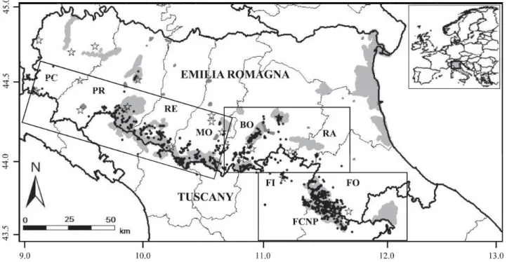
Figure M.3.1. The study area in the Emilia Romagna and Tuscany Apennines in Italy, with locations of the noninvasive wolf samples (filled circles) and wolves found dead (stars). The protected areas are in gray. Rectangles indicate the 3 main sectors of the study area. The eastern sector includes: FI = Florence Province, FO = Forlì-Cesena Province, and FCNP = Foreste Casentinesi National Park. The central sector includes: RA = Ravenna Province, and BO = Bologna Provinces. The western sector includes: MO = Modena Province, RE = Reggio Emilia Province, PR = Parma Province, and PC = Piacenza Province. Longitude and latitude are indicated on the x- and y-axes in decimal degrees (datum WGS84).

21

Individual genotypes for samples were identified at 12 unlinked autosomal canine microsatellites (short tandem repeats [STR]): 7 dinucleotides (CPH2, CPH4, CPH5, CPH8, CPH12, C09.250, and C20.253) and 5 tetranucleotides (FH2004, FH2079, FH2088, FH2096, and FH2137), selected for their high polymorphism and reliable scorability for wolves and dogs. Sex of samples was determined using a polymerase chain reaction (PCR)–restriction fragment length polymorphism assay of diagnostic ZFX/ZFY gene sequences (Caniglia et al. 2012, 2013, and references therein). A panel of 6 STR (FH2004, FH2088, FH2096, and FH2137, CPH2, and CPH8) was used to identify the genotypes with Hardy–Weinberg probability-of-identity (PID) among unrelated individuals, PID = 8.2 x 10-6, and expected fullsiblings, PIDsibs = 7.3 x 10-3 (Mills et al. 2000; Waits et al. 2001)

in the reference Italian wolves.

Another panel of 6 STR (FH2079, CPH4, CPH5, CPH12, C09.250, and C20.253), also selected for their polymorphism and reliable scorability was used to increase the power of admixture and kinship analyses, decreasing the PID values to PID = 7.7 x 10-9 and PIDsibs = 3.1 x 10-4. Maternal haplotypes were identified by sequencing 350 base pairs of the mitochondrial DNA (mtDNA) control region, diagnostic for the haplotype W14, which is unique to the Italian wolf population, using primers L-pro and H350 (Randi et al. 2000). Paternal haplotypes were identified by typing 4 Y-linked microsatellites (Y-STR): MS34A, MS34B, MSY41A, and MS41B (Sundqvist et al. 2001), characterized by distinct allele frequencies in dogs and wolves (Iacolina et al. 2010).

Autosomal and Y-linked STR loci were amplified in 7 multiplexed primer mixes using the QIAGEN Multiplex PCR Kit (Qiagen Inc.), a GeneAmp PCR System 9700 Thermal Cycler (Applied Biosystems, Foster City, California), and the following thermal profile: 94°C for 15 min, 94°C for 30 s, 57°C for 90 s, 72°C for 60 s (40 cycles for scat, urine, and hair samples, and 35 cycles for muscle and blood samples), followed by a final extension step of 72°C for 10 min. Amplifications were carried out in 10-μl volumes including 2 μl of DNA extraction solutions from scat, urine, and hair samples, 1 μl from muscle or blood samples (corresponding to approximately 20–40 ng of DNA), 5 μl of QIAGEN Multiplex PCR Kit, 1 μl of QIAGEN Q solution (Qiagen Inc.), 0.4 μM deoxynucleotide triphosphates, from 0.1 to 0.4 μl of 10 μM primer mix (forward and reverse), and RNase-free water up to the final volume. The mtDNA control region was amplified in a 10-μl PCR, including 1 or 2 ll of DNA solution, 0.3 pmol of the primers L-Pro and H350, using the following thermal profile: 94°C for 2 min, 94°C for 15 s, 55°C for 15 s, 72°C for 30 s (40 cycles), followed by a final extension of 72°C for 5 min. PCR products were purified using exonuclease/shrimp alkaline phosphatase (Exo-Sap; Amersham, Freiburg, Germany) and sequenced in both directions using the ABI Big Dye Terminator kit (ABI Biosystems, Foster City, California) with the following steps: 96°C for 10 s, 55°C for 5 s, and 60°C for 4 min of final extension (25

22

cycles). DNA from scat, urine, and hair samples was extracted, amplified, and genotyped in separate rooms reserved only to low-template DNA samples, under sterile ultraviolet laminar flood hoods, following a multiple- tube protocol (Caniglia et al. 2012), including both negative and positive controls. Genotypes were obtained from blood and muscle DNA, replicating the analyses twice. DNA sequences and microsatellites were analyzed in a 3130XL ABI automated sequencer (Applied Biosystems), using the ABI software SEQSCAPE 2.5 for sequences, and GENEMAPPER 4.0 for microsatellites (Applied Biosystems).

Population structure, assignment, and identification of wolf x dog admixed genotypes

Individual genotypes were assigned to their population of origin (wolves or dogs) using STRUCTURE 2.3.3 (Falush et al. 2003). STRUCTURE was ran with 5 replicates of 104 burn-in followed by 105 iterations of the Monte Carlo Markov chains, selecting the ‘‘admixture’’ model (each individual may have ancestry in more than 1 parental population), either assuming independent or correlated allele frequencies. The optimal number of populations K was identified using the ΔK procedure (Evanno et al. 2005). At the optimal K the average proportion of membership (Qi) of the sampled populations (wolves or dogs) was assessed to the inferred clusters.

Genotypes were assigned to the Italian wolf or dog clusters at threshold qi = 95 (individual

proportion of Membership; Randi 2008), or identified them as admixed if their qi values were

intermediate. Putative wolf x dog hybrids were checked further using additional admixture analyses on observed and simulated genotypes obtained by HYBRIDLAB (Nielsen et al. 2006) and using diagnostic mtDNA and Y-STR haplotypes.

Genetic variability

Based on the assignment tests, all genotypes were grouped as those of wolves, dogs, or hybrids. GENALEX 6.1 (Peakall and Smouse 2006) was used to estimate allele frequency by locus and group, observed (HO) and expected unbiased (HE) heterozygosity, mean (NA) and expected (NE) number of alleles per locus, number of private alleles, and PID and PIDsibs. The polymorphic information content (PIC) was calculated using CERVUS 3.0.3 (Kalinowski et al. 2007). Wright’s inbreeding estimator (FIS; Weir and Cockerham 1984) and departures from Hardy–Weinberg equilibrium were computed using GENETIX 4.05 (Belkhir et al. 1996; 2004). FIS significance was

assessed using 10,000 random permutations of alleles in each population. The occurrence of null alleles was tested in MICROCHECKER (Van Oosterhout et al. 2004). Inbreeding coefficient F of Lynch and Ritland (1999) was estimated using COANCESTRY 1.0 (Wang 2011), with allele frequencies and PCR error rates assessed from the sampled population and 95% confidence

23

intervals (CIs) generated through 1,000 bootstrapped simulations. The sequential Bonferroni correction test for multiple comparisons was used to adjust significance levels for every analysis (Rice 1989). Estimates of variability were express as the mean ± SD.

Identification of packs, pedigrees, and dispersal

All the genotypes that were sampled in restricted ranges (< 100 km2) at least 4 times and for periods longer than 24 months were selected. Their spatial distributions was determined by 95% kernel analysis, choosing band width using the least-squares cross-validation method (Seaman et al. 1999; Kernohan et al. 2001), using the ADEHABITATHR package for R (Calenge 2006) and mapped them using ARCGIS 10.0. According to spatial overlaps, individuals were split into distinct groups that might correspond to packs, for which parentage analyses were performed. The complete genealogy of each group were reconstructed using a maximum-likelihood approach implemented in COLONY 2.0 (Wang and Santure 2009). For each area, as candidate parents all the individuals sampled in the 1st year of sampling and more than 4 times in the same area were considered and as candidate offspring all the individuals collected within the 95% kernel spatial distribution of each pack and in a surrounding buffer area of approximately 17-km radius from the kernel (see ‘‘Results’’). COLONY was ran with allele frequencies and PCR error rates as estimated from all the genotypes, assuming a 0.5 probability of including fathers and mothers in the candidate parental pairs. To be sure that all the possible parentages were detected, the best maximum-likelihood genealogies was compared to those obtained by an ‘‘open parentage analysis’’ in COLONY, using all the males and females as candidate parents, and all the wolves sampled in the study area as candidate offspring. The best maximum-likelihood genealogies reconstructed by COLONY were compared with those obtained by a likelihood approach in CERVUS, based on the Mendelian inheritance of the alleles, accepting only parent–offspring combinations with at most one-twentyfourth allele incompatibilities, and father–son combinations with no incongruities at Y-STR haplotypes. Parentage assignments were determined in CERVUS using natural log of likelihood ratio scores for candidate parents, given the set of candidate offspring genotypes and the allele frequencies in the whole population (when a natural log of likelihood ratio score was positive, the candidate parent is the most likely true parent (Kalinowski et al. 2007). Simulations to determine the likelihood of randomly selected parents was also performed. Natural log of likelihood ratio values that were significant at 95% and 80% thresholds were considered. Natural log of likelihood ratio scores were generated by simulating 10,000 offspring and 50 candidate males, allowing for 20% of the population to be unsampled, 20% incomplete multilocus genotypes, and the genotyping error rate as empirically estimated from the data set (vonHoldt et al. 2008). Values of relatedness (r;

24

Queller and Goodnight 1989) were estimated within and among packs using KINGROUP 2.0 (Konovalov et al. 2004) and compared those with values of 1st order (parent–offspring plus full siblings) and unrelated dyads estimated from 1,000 simulated pairs. A likelihood ratio test was used with a primary hypothesis of r = 0.25 (half siblings or cousins) and r=0.50 (full-siblings or parent– offspring) versus a null hypothesis of r = 0.00 (unrelated) to test for inbreeding within and among packs, at the α = 0.05 level. Locations of individuals in the packs were used in ARCGIS 10.0 to reconstruct the areas and centroids of the 95% kernel spatial distribution for each pack, and the distances between centroids; reconstruct the minimum, median, and maximum distance of genotypes to the pack centroids; and identify dispersing wolves. Individuals sequentially sampled in different territories (> 17 km apart), or that reproduced in a pack different from their natal one were identified as putative dispersers. Individuals that were not assigned to a pack and the dispersers that did not establish in any pack were considered as potential floaters.

Spatial analyses

Fine-scale spatial genetic structure were assessed by multivariate spatial autocorrelation analyses of geographical and genetic distances in SPAGEDI 1.2 (Hardy and Vekemans 2002) and estimated through the autocorrelation kinship coefficient Fij (Loiselle et al. 1995), which is similar to Moran’s I (Smouse and Peakall 1999) but is relatively unbiased even with low sampling variance. Fij was calculated for distance classes that had been determined based on wolves’ home ranges and following recommendations of Hardy and Vekemans (2002). Thus, the equal frequency method was used, which assumes that more than 50% of all individuals were represented at least once in each spatial interval. The 95% Fij CIs and the nonrandom spatial genetic structure were tested via 10,000 permutations and the effects of behavioral biases (sex-biased dispersal and pack relatedness) were investigated by computing autocorrelations separately in males, females, and breeding pairs. Correlations between geographic and genetic distance of individuals and packs were computed after permuting the locations, similarly to a Mantel test (Mantel 1967). Whenever possible, additional field information such as snow-tracking, wolf-howling, camera trapping, and occasional direct observations were used to evaluate the reliability of the inferred pack structure and locations.

25

M.4. Non-invasive genetic sampling to predict species ecological niche and depredation risk

Study area

The study area (71,443 km2) includes the entire wolf range in Italy and is located from the Central Apennines to the Southwestern Alps (7°49’–13°91’ E; 45°–42°39’ N; Fig.1). It shows high habitat diversity as the result of wide altitudinal (from 0 to 2,476 m a.s.l.) and climate (from temperate to continental, to alpine) gradients, landscape morphology, human population density and occurrence of human activities. The upper part of the area is characterized by mountains covered by meadows, pastures and rocky habitats. On the lower mountains and hills, rural ecosystems (mostly abandoned) are turning back into natural shrub lands and deciduous, mixed or evergreen forests. Cultivated fields and artificial surfaces (urban areas, villages, roads, railways) are located in more accessible hills, main valleys, plains and coasts. The environmental heterogeneity, the expansion of natural habitats and re-introduction projects, explain the high diversity of the community of wild ungulates: wild boar, roe deer, follow deer, red deer, and mouflon (Ovis musimon). Domestic ungulates, mostly cows (Bos taurus), sheep (Ovis aries) and goats (Capra hircus), are free ranging in high-altitude pastures from April to October.

Experimental design and wolf presence data

The experiment was carried out using putative wolf samples (saliva, urines, feces, hairs, blood, and muscular tissues from carcasses) collected, from January 2000 to December 2011, along a total of c. 400 trails or country roads averaging about 5.1 km (SD = 2.2) in length and dead wolf sites by more than 150 researchers, students, volunteers and employees of Parks, Forestry Corps and local or national administrations. Scat and tissue samples were individually stored at -20° C in 10 volumes of 95% ethanol; blood sample were stored in a Tris/SDS buffer (see above; Caniglia et al. 2012). Sampling locations were georeferenced in the Universal Transverse of Mercator World Geodetic System (UTM WGS84 32N) coordinate system and then separated in locations collected during the GP and the NGP. The study area was divided into adjacent isometric cells of 5 x 5 km, approximately the resolution chosen in previous studies about habitat suitability modeling for wolves in Italy (Massolo and Meriggi 1998; Marucco and McIntire 2010). In long-term researches, spatial and temporal variations in sampling efforts would inevitably occur. However, the large scale and long duration of a study should overcome this bias and avoid affecting the results in any systematic way (Jedrzejewski et al. 2008). To avoid that GNESFA results could be influenced by differences in seasonal collections sampling effort was estimated in the two periods by Gaussian

26

kernels (Elith et al. 2010). Then, differences in the resulting kernel maps were tested with a Wilcoxon-signed rank test (Phillips et al. 2006; Rebelo and Jones 2010).

Predictor Variables

For the entire study area, data on ecological, topographic, trophic and anthropogenic features were collected (Table M.4.1). Habitat diversity (Shannon Diversity Index) and land cover types were obtained from the Coordination of Information on the Environment (CORINE Land Cover 2006, IV Level; http://www.sinanet.isprambiente.it), the European land cover database. Topographic variables were obtained from a Digital Elevation Model of Italy with a spatial resolution of 20 m (http://www.sinanet.isprambiente.it). From this, aspect, slope and roughness were derived (rugged terrain, topographically uneven, broken, or rocky and steep). Prey species availability and abundance are the main food resources and affect the distribution of wolves. In the analysis the abundance of wild ungulate prey over the study area was included (Carnevali et al. 2009) and the Shannon diversity index for wild prey was calculated, since the occurrence of more than one species influences the wolf habitat suitability (Massolo and Meriggi 1998, Ciucci et al. 2003). The abundance and Shannon diversity Index of domestic prey was derived from the Agricultural Italian Census (http://censimentoagricoltura.istat.it). As human factors, the presence and distance form artificial surfaces, as well as the human and hunter densities were considered (http://dati.istat.it). All variables were re-sampled to a resolution (5,000 m cell size) using ArcGIS 10 (ESRI, Redlands, California).

27

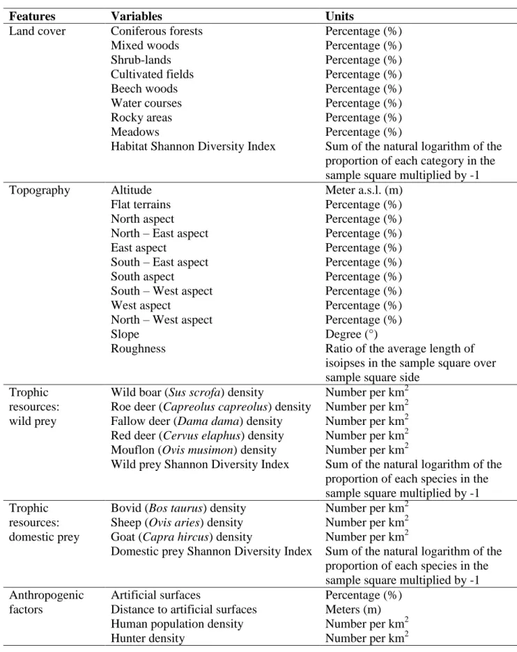
Table M.4.1. Variables used in the General Niche Environment System Factor Analysis.

Features Variables Units

Land cover Coniferous forests Percentage (%)

Mixed woods Percentage (%)

Shrub-lands Percentage (%)

Cultivated fields Percentage (%)

Beech woods Percentage (%)

Water courses Percentage (%)

Rocky areas Percentage (%)

Meadows Percentage (%)

Habitat Shannon Diversity Index Sum of the natural logarithm of the proportion of each category in the sample square multiplied by -1

Topography Altitude Meter a.s.l. (m)

Flat terrains Percentage (%)

North aspect Percentage (%)

North – East aspect Percentage (%)

East aspect Percentage (%)

South – East aspect Percentage (%)

South aspect Percentage (%)

South – West aspect Percentage (%)

West aspect Percentage (%)

North – West aspect Percentage (%)

Slope Degree (°)

Roughness Ratio of the average length of

isoipses in the sample square over sample square side

Trophic resources: wild prey

Wild boar (Sus scrofa) density Number per km2 Roe deer (Capreolus capreolus) density Number per km2 Fallow deer (Dama dama) density Number per km2 Red deer (Cervus elaphus) density Number per km2 Mouflon (Ovis musimon) density Number per km2

Wild prey Shannon Diversity Index Sum of the natural logarithm of the proportion of each species in the sample square multiplied by -1 Trophic

resources: domestic prey

Bovid (Bos taurus) density Number per km2 Sheep (Ovis aries) density Number per km2 Goat (Capra hircus) density Number per km2

Domestic prey Shannon Diversity Index Sum of the natural logarithm of the proportion of each species in the sample square multiplied by -1 Anthropogenic

factors

Artificial surfaces Percentage (%)

Distance to artificial surfaces Meters (m)

Human population density Number per km2

28 Modeling methods

Wolf samples were genotyped following the methods showed in M.3 (Caniglia et al. 2014). The locations of genotyped wolf samples were used to rank each cell as ‘used’ if at least one wolf genotype was sampled within its boundary. Used and available sites were compared (all the cells of the study area) through a niche-based approach, GNESFA. It identified the relations between the availability and utilization distributions with several advantages: it doesn’t rely on any population structure hypotheses (autocorrelation), it extracts non-correlated components, it is especially suited to analyse presence-only data and compute habitat suitability maps (Basille 2008). Two measures of the species ecological niche are provided:the marginality (the direction in which the species differs from the average conditions of the whole area) and the specialization (the ratio between the variance of available conditions and the variance of conditions used by the species; Hirzel et al. 2001; Basille 2008). GNESFA encompasses three complementary analyses: the Factor Analysis of the Niche Taking the Environmental as the Reference (FANTER; Calenge and Basille 2008); the Mahalanobis Distance Factor Analysis (MADIFA; Calenge et al. 2008); the Ecological Niche Factor Analysis (ENFA; Hirzel et al. 2001). The FANTER is centered on the availability distribution and identifies the variables affecting the shape, the central tendency and the spread of the niche relative to the environment considered, showing how the niche in the ecological space differs from the study area; both the first and the last components in the analysis were considered because the formers explained the marginality, whereas the latters the specialization (Calenge and Basille 2008). The MADIFA is centered on the utilization distributions and determines whether the environment is similar to that occupied by the species; the more similar the conditions in a location are to the centroid of the ecological niche (the optimum of the species), the smaller is the Mahalanobis distance (D2) and the more suitable the habitat is at that location (Calenge et al. 2008; Knegt et al. 2011). The mean D2 over the available area was used as a measure of habitat selectivity regarding independent variables and the relationship between D2 and the range considered was analyzed. MADIFA combines marginality and specialization into a single measure of habitat selection (Calenge and Basille 2008). Finally, the ENFA is centered both on the utilization and the availability distribution (Calenge and Basille 2008); marginality is fully explained by the first factor, while specialization by the others. For further details, see Calenge and Basille (2008).

Wolf potential distribution, model validation and predation risk

Wolf locations were bootstrapped with replacement 1,000 times a season to obtain potential distribution maps estimated by MADIFA, the best method in the GNESFA framework to compute appropriate suitability maps (Calenge et al. 2008). To provide an assessment of MADIFA’s power,

29

the predicted values were compared with the real ones through the use of (i) Receiver Operator Characteristics (ROC) curves (Fawcett 2004; Ko et al. 2011), (ii) correct classification rate (CCR; Ahmadi et al. 2013), (iii) Cohen’s kappa (k) (Manel et al. 2001) and (iv) the Boyce’ Index (B) (Boyce et al. 2002; Jones-Farrand et al. 2011). Combining MADIFA’s predictions, the wolf average (± SD) potential distributions was calculated. Assuming that an increase in wolf suitability corresponds to an increase in depredation risk (Kaartinen et al. 2009; Marucco and McIntire 2010), the risk probability of pastures was estimated by calculating the probability of wolf presence during the GP in all meadows available for livestock breeding.

The statistical analyses presented here were computed in the open-source software R (http://www.R-project.org/).

30

M.5. Landscape-genetics and habitat suitability models: general implications of a specific application

Data set on Italian wolves

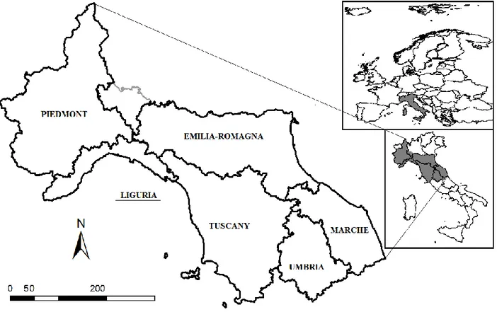
The data set originated from an area of 97,044 km2 from the Central Apennines to the Western-Central Alps in Italy (6°62’–13°91’ E; 46°46’–42°39’ N; Fig. M.5.1).

Figure M.5.1. Study area in Italy (black lines indicate regional borders, grey line indicates the border of the province of Pavia, in the Lombardy region).