Landscape analysis and assessment for the management of agricultural non point pollution sources

UNIVERSITÀ DEGLI STUDI DELLA TUSCIA DI VITERBO

DIPARTIMENTO DI INGEGNERIA AGRARIA E AGRONOMIA DEL TERRITORIO Università degli Studi di Napoli Federico II - sede consorziata

CORSO DI DOTTORATO DI RICERCA

Scienze e tecnologie per la gestione forestale ed ambientale XXII Ciclo

Landscape analysis and assessment for the management of agricultural non point pollution sources

Coordinatore: Prof. Gianluca Piovesan

Tutor: Prof. Lorenzo Boccia

agricultural non point pollution sources

1. Introduction ... 1

1.1. The context ... 1

2. Agricultural non point pollution sources... 5

2.1. Nitrate directive ... 5

2.2. Agricultural “wastes” ... 6

2.3. Campania region context... 10

3. Materials and methods... 15

3.1. GIS... 15 3.2. Geostatistics... 18 3.3. GLEAMS... 26 3.4. Samples analysis... 28 4. Landscape management... 32 4.1. Rural landscape ... 32 4.2. Landscape structures ... 33

4.3. The buffer zone concept ... 39

4.4. Management issues... 42

5. Nitrate leakage in a high buffalo district (Caserta province)... 46

5.1. Introduction ... 46

5.2. Materials and methods... 47

5.3. Results and conclusions... 48

5.4. References ... 51

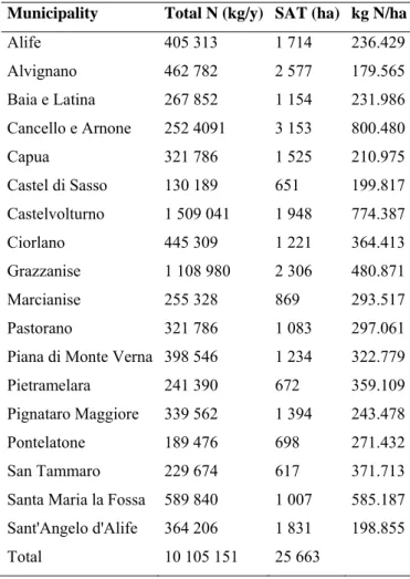
6. Spatial assessment of animal manure spreading and groundwater nitrate pollution... 52

6.1. Introduction ... 52

6.2. Materials and methods... 55

6.2.1. Study site ... 55

6.2.2. Nitrogen fertilization ... 57

6.2.3. Site surveys... 59

6.2.4. Spatial analysis of nitrogen production ... 60

6.2.5. Spatial analysis of groundwater nitrate concentration... 61

6.3. Results ... 64

6.4. Discussion... 70

6.5. Conclusion... 75

6.6. References ... 77

7. Impacts of Bubalus Bubalis manure on agronomic management ... 80

7.1. Introduction ... 80

7.2. Materials and methods... 82

7.2.1. Assessment of nitrate leaching considering the local context and the agronomic practices... 82

7.2.2. Monitoring water from wells... 84

7.2.3. Manure sampling ... 85 7.2.4. Geostatistics study ... 86 7.3. Results ... 90 7.4. Discussion... 95 7.5. Conclusion... 96 7.6. References ... 98

8.3. Indexes to define wetlands’ spatial distribution ... 104

8.4. Material and Methods... 108

8.4.1. Site description ... 108

8.4.2. Material... 108

8.4.3. Definition of variables and indexes... 111

8.4.4. Definition of hydric soils... 113

8.4.5. Calibration of the indexes... 114

8.5. Results ... 114

8.5.1. The influence of the Strahler order... 116

8.6. Discussion... 120

8.7. Conclusion... 124

8.8. References ... 125

9. Conclusions ... 129

1.

Introduction

1.1. The context

It is increasingly recognized that more sustainable approaches are needed for planning and managing landscapes and environment in a general approach.. The spatial dimension of sustainability engages processes and relations between different land uses, ecosystems at different scales, and over time (Botequilha et al., 2002 ).

The success of landscape planning and environmental management strategies depends largely on the congruence between the operational scales of landscapes and the spatial scope of the planning instruments (Diaz-Varela et al., 2009).

Environmental management is a process of decision-making that considers all the different variables and processes that characterize the environment as a whole. Risk assessments, precautionary principles, adaptive management and scenario approaches are adopted to deal with the uncertainty of nature.

The management of environmental issues is complex. Many optimization models exist but generally there is a knowledge gap in linking all the environmental variables and objectives.

Considering natural variables, landscape features, climate, land use, land cover and all the environmental constraints is a challenge in developing management plans and strategies. Uncertainty and variability are the main feature of this big challenge. As an example, as agricultural systems become more complex, multiple objectives that are in conflict with each other need to be addressed. Competition for scarce resources by different enterprises is a major concern in many agricultural production systems. Competition occurs at farm level e.g. between different crops as well as regional level, where utilization of scarce water resources for agricultural purposes often comes into

conflict with the requirement for in stream ecosystem services. For example, in agriculture systems conflict may arise from maximizing economic returns (i.e. net revenue) as opposed to minimizing the use of resources such as water, fertilizer applications. On the other hand, minimizing costs rather than maximizing net revenue may also be important in some water management systems. Under these conditions, multiple criteria decision-making techniques (MCDM) are useful tools to explore different management options.(Xevi and Khan, 2005). The success of multi-objective planning will depend on clear goal definition. If goals and objectives are not articulated at the outset, there will be no criteria for assessing the suitability of specified actions. Having set objectives, it is then necessary to identify, for each one, the elements that are required in a landscape, the quantities or area required, their distribution in the landscape, and the appropriate management regime. If these requirements can be determined, they must be combined in a way that addresses all objectives (Lambeck, 1999).

Furthermore, focusing on water compartment, for example, in most Mediterranean countries groundwater is the primary resource for irrigation and drinking. Nowadays, scarcity of water is a limiting factor for sustainable growth. Therefore, preserving its availability and quality is a key issue. Excessive groundwater withdrawal is a risk factor, because it causes sea-water intrusion phenomena resulting in progressive groundsea-water salinization, which is particularly damaging for agriculture.

Generally speaking, making decisions in a situation where environmental risk is involved is a political action based on information collected during risk assessment. Therefore, the evaluation of environmental risk due to anthropic activities is an important step in mitigating the impact of such activities on natural resources and in recreating the co-evolutionary process between human and natural components of the environment. A territory is, in fact, the result of a stratification process characterized by the

outputs of complex interrelationships between anthropic activities and sites. Among such activities, agriculture is surely one of the most relevant. However, massive soil exploitation, continuous groundwater withdrawal and the use of fertilizers and pesticides have a significant negative impact on the environment. Finding out how compatible a specific anthropic development is with environment conservation by assessing its impact on natural resources is a key step towards understanding the interactions between territory and local activities. In this context, environmental risk assessment and management represent a useful tool for describing local conditions characterized by a high degree of environmental risk. Risk assessment can be defined as the process of estimating the possibility that a particular event may occur under a given set of circumstances. Risk management, on the contrary, is the process in which decisions aimed at reducing risk and preserving public health and environmental resources are made, using information gathered during the assessment phase. Thus, environmental risk assessment could be considered as the basis of a decision making process (i.e. risk management) (Uricchio et al., 2004).

Starting from the concept that, nowadays, many farms are not sustainable in their current form, even if this industry has generated significant wealth, it has also created major problems in the form of land degradation, pollution, loss of biological diversity. Because these processes cannot be managed by individual land-holders acting in isolation, it is essential that there be a shift from traditional farm-based, single-objective land management, to multiple-goal, sustainable management practices implemented at catchment or regional scales.

By the context described above, agricultural activities play a main role in influencing a sustainable development. For example, focusing on farming, the large quantities of slurry and manure that are produced where animals are raised, could be an important source of organic matter and nutrients for

agriculture. The use of these wastes via land application, after opportune treatments, could improve physical properties of soil, such as soil porosity, water holding capacity. For this reason, the application manure could be beneficial for soil conservation, especially in degraded soils and soils susceptible to erosion, although the response to soil amendment is soil-site specific. Obviously, the benefits of manure may be partially offset by the risk of water pollution associated with runoff and leaching from fields, especially if rainfall occurs shortly after application.

Ramos et al. (2006) reported that the application of manure to the fields has implications for erosion processes. When manure is applied on the soil surface, the quantity of eroded material decreases but runoff can increase by up to 30%. Hence the pollution of surface water can increase and, if rainfall takes place within a short period after application, faecal coliforms in runoff waters reach high concentrations, exceeding the standards for bathing water quality, especially because they are transported in association with organic matter particles rather than linked to the soil or suspended in water (Ramos et al., 2006).

This thesis study tries to product a general framework of the issues concerning agricultural non point pollution sources, their management and their connection with the landscape. Particularly, the thesis focuses on an area in south Italy where livestock activities are intensive and the consequent manure has to be managed. Further, studies about landscape assessment were developed focusing on Brittany region (France).

The aim of the thesis researches is to have a clear idea of the environmental problems connected to agricultural non point pollution sources in the areas mentioned above and to identify a way to manage and reduce this kind of pollution.

2.

Agricultural non point pollution sources

2.1. Nitrate directive

In 1991, the council of environmental ministers of the European Union (EU) adopted the council directive concerning the protection of waters against pollution caused by nitrates from agricultural sources, 91/676/EEC (European Commission, 1991). The directive aims at reducing and preventing water pollution caused by nitrates from agricultural sources. Before the end of 1993, member states were obliged to identify so-called ‘vulnerable zones’ and establish good agricultural practices. These should require that farming be practiced in a way that minimizes the pollution of water by nitrates. These should specifically result in nitrate concentrations in groundwater not exceeding 50 mg NO3−/l.

To realize the objectives of the directive, member states established Action Programs, that should include rules for (1) the periods in which the use of certain types of chemical fertilizer are prohibited, (2) the storage capacity for, or the disposal of, livestock manure and (3) limitation of land application of fertilizers. More specifically, account should be taken of local characteristics such as soil conditions (type and slope), climatic conditions and irrigation and balancing N supply with crop N demand, including both chemical fertilizer and manure. Action Programs should also ensure that the amount of livestock manure applied does not exceed the equivalent of 170 kg N/ha, corresponding with 2 livestock units per ha.

Moreover, member states were allowed to derogate from this standard, but only on the basis of objective criteria relating to crop and soil characteristics. Some examples of criteria have already been provided in the directive, such as a long growing season, crops with a high N uptake, high net precipitation and soils with a high denitrification capacity (Sonneveld et al, 2003).

In this context many control and assessment plans were developed. For example to control and prevent nutrient pollution from agricultural non-point sources, the Dutch government introduced the Mineral Accounting System (MINAS) in 1998, a nutrient bookkeeping system which taxes farms with nutrient surpluses exceeding safe threshold values. Moreover, reducing surpluses is assumed to be most effective through an improvement of management. Changing farm management rather than farm structure can therefore reduce nutrient surpluses more effectively, making it a more interesting approach for policy makers. (Ondersteijn et al., 2003).

Even if the directive 91/676/EEC has been in operation since 20 years ago, most of the constraints defined by the directive have been largely not respected by the member states. The main obligations not completely respected are the application of the so called “Action Programmes”, the management of the monitoring campaigns to verify water quality in terms of nitrate concentration, the identification of the vulnerable zones.

2.2. Agricultural “wastes”

Organic wastes are typically products of farming, industrial or municipal activities, and are usually called ‘‘wastes’’ because they are not the primary product. However the goal is to make the ‘‘waste’’ a resource that can be utilized and not just discarded. Possible uses of organic wastes include use as fertilizer and soil amendment, energy production, and production of chemicals (volatile organic acids, ammonium products, alcohols). Agriculture has traditionally used animal manures for fertilizer and improving soil physical and chemical properties. Utilization of various organic wastes in agriculture depends on different factors, including the characteristics of the waste such as nutrient and heavy metal content, energy value, odor generated by the waste, availability and transportation costs, benefits to agriculture, and regulatory considerations. Further considerations about this context regard:

regional imbalances of nutrients (e.g., not enough land on the farm to apply nutrients produced by animals on the farm), imbalance of nutrients in waste compared to crop needs, the alternative use of chemical fertilizers, the variability in nutrient content, satisfying environmental regulations on application amounts, application timing, and application methods, and possible environmental concerns, such as emission of ammonia and other gases, odor, and pathogens. One of the alternative management strategy could be changing animal feeding in a way to convert final outputs (mainly manure) into higher value resources. In addition, potential transport of pathogens via air or water, and environmental air quality concerns with emissions of ammonia, methane, hydrogen sulphide, nitrous oxide, and odorants can result in more regulations, and lead to alternative treatment schemes, which can change the nature of the organic wastes that are applied to land or used in horticulture uses. Concerns for animal welfare and development of innovative energy policies also have potential to affect changes in management of manure and other organic materials. Some of the manure management/treatment systems are discussed in publications such as Burton and Turner (2003).

Several challenges for utilizing organic wastes for soil amendment and fertilizer value exist. These challenges are linked to the possible environmental impacts which may result from land application of animal manures and other organic wastes. Among these impacts the most frequent are the emission of greenhouse gases, emission of bad odors, production of pathogens, the water pollution by nitrogen, phosphorous, organic matter and pathogens, heavy metals soil accumulation.

Suitable equipment and management are thus required. One of the most critical and important aspect is how the application rates are determined. If application rate of animal manure is based on nitrogen, then phosphorus is usually applied in excess of crop uptake, because of the difference in the N:P

ratios which exist between the manure content (about 3:1) and the crop requirement (about 8:1). A management option to address excessive N, P, Cu and Zn application to land may include diet manipulation strategies to reduce intake and increase digestibility and absorption of these compounds by the animals, thus producing less nutrients in manure. When the farm produces excessive nutrients for application on-farm, then treatment options can be added to reduce N (e.g., by conversion to dinitrogen gas) or partition nutrients into more concentrated or stable forms that can be transported elsewhere. For reduction in pathogens, lime treatment or high temperature aerobic or anaerobic treatment is required to essentially eliminate pathogens. To reduce odor, aeration treatment offers a viable, but somewhat expensive option. Also, different land application techniques are used to reduce odor and ammonia emission, such as injection.

Composting is a good strategy to move nutrients off farm. By composting, a more valuable resource can be obtained, but markets must be developed and farmers must determine the extra processing to be manageable and economically viable. There is also the possibility of a centralized composting facility that serves several farms. Composting can emit ammonia and other gases of concern to the atmosphere, requiring consideration for collecting and/or treating off-gases.

In some cases, energy recovery from anaerobic or aerobic digestion of organic wastes can be beneficial for certain objectives, but may have minimal benefit for nutrient management (Burton and Turner, 2003). Nutrient content generally remains unchanged, but nutrient availability may be increased and soluble organic matter reduced. Another benefit can be reduction of odor. The energy can be used on-farm or sold. If government energy policies were improved to support more ‘‘green energy’’ production, then more farms might consider anaerobic digestion for manure treatment and energy recovery.

Inherent in considering alternative management schemes for organic wastes are the costs and benefits. If regulations or environmental factors require additional treatment that increases costs of production and operation, then the farmer loses profit unless costs are shared with the government or other agencies. It is not easy to determine environmental costs and benefits of alternative waste management policies. Government can offer incentives such as cost sharing of equipment or guarantee of not changing regulations for a period of time for improved waste treatment.

Economics may also suggest that a cooperative or regional facility is needed for certain waste management schemes. However, farmer and public acceptance of this is important because odor from large treatment plants and transportation of organic wastes on public roads may present more community concerns, and farmers may choose other alternatives if the regional treatment system is not clearly advantageous both economically and for management efficiency. Utilization of organic wastes occurs more easily if there are clear economic incentives. Better organization through farmer cooperatives, organic waste sellers, and government or other agencies could improve the economics. At least initially, more government subsidies may be needed to help distribute nutrients over a larger region by helping with transportation or costs of further processing (Wasterman, 2005)

As a result of relatively more successful control of point sources of nutrients, agricultural nonpoint sources remain the most important contributor of nutrient loads impacting the quality of water resources (USEPA, 2000). The impact of nutrients on the quality of US water resources has been widely documented. Various studies have shown that eutrophication of freshwater depends on the inflow of nutrients, mainly nitrogen (N) and phosphorus (P), from land uses above the body of water. Elevated levels of P have been consistently identified as the most important source of nutrient-induced freshwater quality problems. Due to various biochemical processes, P tends to

be the limiting nutrient in the growth of algal forms in rivers and lakes. Thus, excessive P loadings are a significant factor in the eutrophication of some receiving waters. Nonpoint source pollution problems have been attributed in part to conventional tillage practices that lead to increased soil erosion rates and associated sediment-bound nutrient losses, because of the inversion of most or all of the crop residues into the soil. Similarly, fertilizer and manure placement methods have been identified as potential factors impacting water quality. Notwithstanding the impacts of conventional tillage methods, various studies have found that plowing or disking fertilizer into the soil could reduce losses in runoff (Osei et al., 2003).

2.3. Campania region context

The Campania region is situated in the southern Italy, west coast (Fig.2. 1).

The region engendered great interest mainly because it appears as a lab area for the studies about agricultural non point pollution sources and their management.

The regional surface is 13 600 km2. The territory is characterized by the 50% of hills and 35% of mountains. In 2000 (V Agricultural Census) the SAU was about 590 000 ha representing the 43% of the total surface. In 2005 the SAU decreased until 560 000 ha, first because of agricultural activities abandonment. The main feature of the farms in Campania region is their small dimension (the 40% of the farms is characterized by a surface smaller than 1 hectare, ISTAT 2005). Thus, the decrease of the SAU corresponds to a decrease in number of the smallest farms and, consequently, to a development and increase in surface of the biggest farms.

In 2005 the 37% of the farms’ surface was used for arable fields, the 21% for woods and the 14% for grazing.

Data collected in 2005 report that the 11% of the Italian livestock farms are in Campania. The comparison between the number of animal heads,

mainly bovine and buffalo, in 2003 and 2005 shows an increase of about 10%. Whereas, in the same period, the number of livestock farms decreased (-20%). In 2007 the number of buffaloes and bovines was 480 000 (National Data Bank BDN, 2008).

In 2000-2004 the value-added by agriculture in Campania was the 4% of the total value added in the region. It was then characterized by an increase in 2003-2005 (+4,5%).

Agricultural activities involve the 5% of the regional workforce that corresponds to the 9% of the national datum (SeSIRCA elaborations 2005).

Several studies were carried out to quantify the non point pollution in Campania. They revealed that there were areas where nitrate concentration in water was great (Fig.2. 2, Onorati et al., 2003). The use of synthetic nitrogen fertilizers (600 kg/ha per year only in the province of Naples) was higher than the national average use. This contributed to the ground water pollution. In Caserta province the great fertilizers’ use (about the 100% of the total mineral fertilizers) determined the increase of the pollution of the deeper ground water. Furthermore, the presence of high chloride content in the same samples, where nitrate content was high, involved the pollution by manure. This is perfectly coherent with the agricultural and livestock activities of the region, especially in particular areas such as the Caserta province (Infascelli et al, 2007 and 2009).

Basing on the European and National legislations (mainly Nitrate Directive and Italian Legislative Decree 152/99 and Ministerial Decree 7th April 2006) and on monitoring campaigns in Campania, the Region defined the vulnerable zones to agricultural nitrate (DGR 700/03) and many other regional programs (i.e. Programma d’azione per le zone vulnerabili all’inquinamento da nitrate di origine agricola) in order to obtain good guides lines for monitoring and checking and managing nitrate pollution. The Region identified 115 000 ha of vulnerable zones to agricultural nitrate.

The Region studies and the consequent measures and directive adopted, are all based on deep studies of the territory features. Among these, the soil and hydrogeological studies, conducted by Allocca et al.(2003) and by the Campania Region (www.sito.regione.campania.it/agricoltura/pedologia/home.htm), provide maps and information fundamental to characterize and to determine the connections between the several aspects that take part into the environmental and anthropic processes, such as farming.

a)

b)

3.

Materials and methods

3.1. GIS

Spatial issues such as the identification of sensitive areas, the determination of the degree of site suitability and the calculation of the waste application rate for various spatial locations can be resolved using a geographic information system (GIS). A GIS is a computer-assisted system for acquisition, storage, analysis and display of geographic data. It is also possible to combine a range of different kind of factors (biophysical, environmental, social, economic) to produce a planning output. The GIS is also capable of combining spatial and non-spatial data to produce a map with site-specific outputs. For instance, the spatial parameters (e.g. crop distribution and site suitability maps) could be combined with the non-spatial parameters (e.g. crop nutrient requirements) using a map algebra. With the availability of manure nutrient contents, the plant nutrient requirement map could also be translated into a manure application rate map using a similar algebraic function within the GIS.

Agricultural, environmental, and/or socio-economic problems may arise where the rate of animal waste application to agricultural fields is determined on a limited range of factors. For instance, using manure to meet the requirements of a single plant nutrient may not necessarily satisfy the requirements for other nutrients, or may lead to run-off and leaching losses to the environment. Moreover, it may direct manure application to inappropriate sites resulting in odour or economic viability problems. For example the rate of animal waste application within agricultural fields is generally based on the crop requirement for either nitrogen (N) or phosphorus (P). However, excess P may be applied to soils where the manure application rate is based solely on the nitrogen content. Excessive application of P is a serious environmental

concern because it is the single most important nutrient influencing eutrophication and toxic algae blooms (Leone, 2004).

Therefore, there is a need for site-specific judgement in determining the manure application sites and rates. The site-specific judgements include excluding totally unsuitable areas from animal waste application, varying application rates on suitable areas based on site-specific requirements, and using measures to minimise any environmental impacts of animal waste application on marginally suitable areas (Badri B. Basnet et al., 2002).

GIS, supported by computer development, allows for a complete spatial analysis to solve problems in planning. Each project of environmental assessment has to be supported by data and information that are integrated into the territory context. An Information Geographic System allows the possibility to view, understand, question, interpret, and visualize data in many ways that reveal relationships, patterns, and trends in the form of maps, globes, reports, and charts. This is the reason why GIS technology should be integrated into any farm information system framework: it can be updated and used as support for assessment, review and monitoring actions that aim to pursue environmental and management targets.

In order to plan and monitor the environmental problems, the assessment of hazards and risks becomes the foundation for planning decisions and for mitigation activities. GIS supports activities in environmental assessment, monitoring, and mitigation and can also be used for generating Environmental models.

Enormous variety of environmental data is generated from different sources. GIS is a powerful tool to analyse the present environmental scenario and also to project the future. Some of the examples where GIS can be effectively used are in environmental planning, ground water contamination, water quality, waste management, air and water pollution, natural hazards and their mitigation etc.

GIS is one of the key tools in the environmental management. It can moreover be a communication tool of environmental information between the public and policy makers since it is the technical basis for the multimedia approach in environmental decision-making.

GIS is a powerful tool for environmental data analysis and planning. GIS stores spatial information (data) in a digital mapping environment. A digital map can be overlaid with data or other layers of information onto a map in order to view spatial information and relationships. GIS allows better viewing and understanding physical features and the relationships that influence in a given critical environmental condition. Factors, such as steepness of slopes, aspects, and vegetation, can be viewed and overlaid to determine various environmental parameters and impact analysis.

GIS can also display and analyze aerial photos. Digital information can be overlaid on photographs to provide environmental data analysts with more familiar views of landscapes and associated data.

A geographic information system (GIS) integrates hardware, software, and data for capturing, managing, analyzing, and displaying all forms of geographically referenced information. It allows territorial, but also logic and conceptual analysis.

The only location can not represent a real information, but if numeric, alphanumeric, statistical data are added the geographical datum becomes an information. A GIS stores data and information as thematic layers that can be linked one to each other. A first important distinction to make is between datum and information. the datum is the numeric entity that identify the characteristics of the studied process; the information is the datum reprocessing in order to be able to spatial represent the original datum or to produce new information. For example a DEM can be elaborated to obtain new information such as the slope, the exposure, the altimetry and other (Leone, 2004).

Some of the GIS application fields are: territorial and landscape planning, environmental assessment and monitoring, controlling agricultural production, etc.

3.2. Geostatistics

Natural and environmental phenomena, in general, are typically distributed in space and/or time, characterized by high variability, number and variety. Knowledge of attribute value has little interest unless location and /or time measurement are known for the data analysis. Thus, classical statistics might be too expensive and limiting in dealing with these issues. Geostatistics provides a set of statistical tools for incorporating the spatial and temporal coordinates of observations in data processing.

The development of geostatistics began in 1960s as a methodology for estimating recoverable reserves in mining deposits. Until 1980s it was mainly viewed as a means to describe spatial patterns and interpolate the value of an attribute of interest at unsampled location Today it is extensively used in the mining and petroleum industries, and in recent years has been successfully integrated into remote sensing and GIS. Geostatistic is now increasingly used to model the uncertainty about unknown values through the generation of alternative images that all honour the data and reproduce aspects of the patterns of spatial dependence or other statistics deemed consequential for the problem at hand. A given scenario or transfer function can be applied to the set of realizations, allowing the uncertainty of the response to be evaluated.

There are often only few measurement of the attribute of interest. The resultant predicted maps thus provide poor resolution and the corresponding uncertainty may be very large. In such situations it is critical to deal with information that is more densely sampled, even if further data are achieved by indirect yet exhaustive information or integrated through secondary data in prediction and simulation algorithms.

Geostatistics deals with spatial data, i.e. data for which each value is associated with a location in space. In such analysis it is assumed that there is some connection between location and data value. From known values at sampled points, geostatistical analysis can be used to predict spatial distributions of properties over large areas or volumes.

Statistics generally analyzes and interprets the uncertainty caused by limited sampling. For example, a conventional statistical analysis of core samples from a site investigation program might show that measured cohesion values of a material can be described by a normal distribution. However, this distribution only describes the population of values gathered in the investigation; it does not offer any information on which zones are likely to have high cohesion values and which areas low values. Geostatistical analysis, on the other hand, interprets statistical distributions of data and also examines spatial relationships. For the example given, it is capable of revealing how cohesion values vary over distance, and of predicting areas of high and low cohesion values. The discipline provides tools for capturing maximum information on a phenomenon from sparse, often biased, and often under-sampled data. Ultimately it produces predictions of the probable distribution of properties in space.

Geostatistics, as mentioned above, is a collection of statistical methods which were traditionally used in environment science. These methods describe spatial autocorrelation among sample data and use it in various types of spatial models. Geostatistics changes the entire methodology of sampling. Traditional sampling methods don't work with auto-correlated data and therefore, the main purpose of sampling plans is to avoid spatial correlations. In geostatistics there is no need in avoiding autocorrelations and sampling becomes less restrictive. Also, geostatistics changes the emphasis from estimation of averages to mapping of spatially-distributed populations.

Detailed description of most geostatistical methods can be found in Isaaks and Srivastava (1989) and Goovaertes (1997) .

A first step, in the aim of a good geostatistics response, is to avoid excessive data skewness. Thus, in case of asymmetric distribution of data, a good practice should be handle the extreme values by removing them, if not representative; classifying them in separated classes; using descriptive statistics more robust than the common mean value and the standard deviation (i.e. semivariogram, relative semivariogram, correlation coefficient etc.); transforming data through functions such as logarithmic or square root function.

A tool widely used to measure the degree of correlation between the values of a same attribute in two different locations, at distance h, is the scattergram. Moreover, spatial autocorrelation can be analyzed using covariance functions, correlograms and variograms (or semivariograms), which have the following mathematical equations:

( )

_{( )}

(

)

∑

( )

( )

( )

_{( )}

[

( ) (

)

]

∑

where z(xi) is the value of the attribute z at the point xi ; h is the measurement

distance (so called lag distance); N(h)is the number of data pairs at distance h;

m is the expected value; s is the standard deviation.

random functions: in the study area the attributes vary following a specific probability distribution function, whose characteristic parameters are known (i.e. mean value and variance for a normal distribution).

Regionalized variables: they are random variables z(x) defined in space. Considering all the possible values that z(x) can assume in each point a random function Z(x) is obtained. All the random variables that form the random function Z(x) have the same cumulative probability distribution F(z) independent that does not depend on the location x:

F(x1…xN;z1…zN ) = Prob { Z(x1)<z1….Z(xN)<zN }

Stationarity: the random function Z(x) is said to be stationary within the study area if the correspondent F(z) is invariant under translation:

F(x1…xN;z1…zN )= F(x1+h…xN+h;z1…zN )

Stationarity is not a characteristic of the phenomenon under study, rather a decision made by user for the random function model. A random function is said to be stationary of order two when its expected value E{Z(x)} exists and is invariant within the study area and the spatial covariance C(h) exists and depends only on the separation vector h. Thus with h=0,

C(0)= E{(Z(x)-m)2}=s2

where s2 is the sampling covariance.

The semivariogram (γ(h)) is the tool used to model the degree of spatial dependence between data separated by a vector h:

( )

_{( )}

[

( ) (

)

]

_∑

where z(xi) is the variable value at xi, h is the lag distance, N(h) is the number

of data pairs at distance h.

The semivariogram provides information about the spatial continuity and variability of the data. Generally, the semivariogram increases with the distance h, until a constant value called sill at a distance called range (Fig.3. 1).

The sill corresponds to the sampling variance s2, thus observations out of the range are not spatially correlated. The semivariogram value may not tend to zero when h tends to zero, although by definition γ(0)=0. Such a discontinuity is called nugget effect.

LAG DISTANCE S E M I V A R I A N C E

Fig.3. 1Semivariogramfeatures

It is mainly due to measurement errors and/or spatial sources of variation at distances smaller than the shortest sampling interval.

The semivariogram can be approximated by some mathematical model (Fig.3. 2):

( )

II) Spherical model

a

h>

( )

[

(

)

]

III) Esponential model

( )

[

(

)

]

0 C1 exph a

C h

γ = + −

In these equations h is the lag distance, a is the range, C0 is the nugget effect

and C0+C is the sill.

Fig.3. 2 Typical models of semivariogram

If data have intrinsic stationarity, that is the semivariance between two points depends only on the magnitude and the direction of h vector and not on positions, and if data have the second order stationarity, the semivariogram can be expressed as:

γ (h)= C(0) - C(h)

Thus the semivariance is expressed in terms of spatial covariance, that is autocorrelation C(h) between data and sampling covariance C(0).

Semivariogram/Covariance modeling is a key step between spatial description and spatial prediction. The main application of geostatistics is the prediction of attribute values at unsampled locations (kriging). The empirical semivariogram and covariance provide information on the spatial autocorrelation of datasets. However, they do not provide information for all possible directions and distances.

The kriging interpolator is a least square linear regression algorithms that account for data related solely to the continuous attribute being estimated. It provides optimal and unbiased predictions of the regionalized variable,

basing on sampling data and on the structural analysis of the data obtained by the semivariogram.

The basic linear regression estimator is defined as:

( ) ( ) ( )

[

]

∑

where λi(x) is the weight assigned to datum z(xi); m(x) and m(xi)are the

expected values; N is the number of data next to the position x to be estimated.

All flavours of kriging share the same objective of minimizing the estimation or error variance σ2E (x) under the constraint of unbiasedness of the estimator; that is:

Min! 2

( )

[

]

E = −

σ x Z x x

under E

[

]

The kriging estimator Z*(x) varies depending on the pattern used to model the random function Z(x).

Usually, a random function can be modelled as: Z(x)= R(x) + m(x)

where R(x) is a residual component and m(x) is a trend component.

R(x) is modelled such as

E[R(x)] =0;

Cov[R(x), R(x+h)]=CR(h)

Thus the expected value of Z at location x is the value of the trend component at that location:

E[Z(x)] = m(x) Three main kriging typologies exist:

Simple kriging. It considers the mean m(x) as known and constant within the study area. Thus the estimator is:

Ordinary kriging. The mean value m(x) is supposed to locally vary and to be stationary within local neighbourhood of the study area:

[

]

∑

∑

∑

The weights λi have to be determined under the following constraints:

thus Σλ

E

[

Z

*

(

x

)

−

Z

(

x

)

]

=

0

minimization of

σ

( )

x

=

Var

[

Z

*

(

x

)

−

Z

(

x

)

]

Thus the estimator becomes:

) ( ) ( * 1 i N i iz x x z

∑

λ

Universal kriging. The mean value is considered unknown and variable within the entire study area. The trend component is modelled as linear combination of fk(x) functions:

∑

ak are the coefficients constant but unknown. By convention f0(x)=1,

thus the estimator is equivalent to the case of an ordinary kriging. The general propriety of a kriging estimator are the following:

- The obtained solution is unique;

- The kriging variance is the smallest obtainable; - The estimator is unbiased;

- The estimator is an exact interpolator

- The kriging is based on the structural analysis of data

- The precision of the prediction can be described by the kriging variance that is determined within all the estimation domain. Hence, it is possible to obtain error maps of the prediction.

3.3. GLEAMS

GLEAMS (Groundwater Loading Effects of Agricultural Management Systems) was developed to simulate edge-of-field and bottom of root zone loadings of water, sediment, pesticides and plant nutrients from the complex climate soil management interactions. Its beginning was in 1984 and it has been updated and evaluated in different climatic region of the world during all this period.

GLEAMS is a continuous simulation, field scale model, which was developed as an extension of the Chemicals, Runoff and Erosion from Agricultural Management Systems (CREAMS) model. GLEAMS assumes that a field has homogeneous land use, soils, and precipitation. It consists of four major components: hydrology, erosion/sediment yield, pesticide transport, and nutrients. GLEAMS was developed to evaluate the impact of management practices on potential pesticide and nutrient leaching within, through, and below the root zone. It also estimates surface runoff and sediment losses from the field. GLEAMS was not developed as an absolute predictor of pollutant loading. It is a tool for comparative analysis of complex pesticide chemistry, soil properties and climate. GLEAMS can be used to assess the effect of farm level management decisions on water quality.

GLEAMS can provide estimates of the impact management systems, such as planting period, cropping systems, irrigation scheduling, and tillage operations, on the potential for chemical movement. Application rates, methods, and timing can be modified to account for these systems and to reduce the possibility of root zone leaching. The model also accounts for varying soils and weather in determining leaching potential.

GLEAMS can be useful in long-term simulations for pesticide screening of soil/management. The model tracks movement of pesticides with percolated water, runoff, and sediment. Upward movement of pesticides and plant uptake are simulated with evaporation and transpiration. Degradation

into metabolites is also simulated for compounds that have potentially toxic by-products. Erosion in overland flow areas is estimated using a modified Universal Soil Loss Equation.

GLEAMS Version 3.0 is written mainly in Fortran 77 with some recent modifications in Fortran 99. It can be operated in batch mode which allows specifying data, parameter, and output file names in the batch file rather than entering the filenames as prompted in interactive mode. The batch file named TEST is provided for user information. This file was used to execute GLEAMS30 with the sample data and parameters and generate the sample output files. The order of the files as shown is essential. If only the hydrology and erosion components are to be run, then the pesticide and nutrient parameter files and output files should not be included in the batch file. Likewise, if hydrology, erosion and pesticides are run, the nutrient parameter and output files should not be listed. If selected variables are not specified (in the hydrology parameter file), the selected output file can be eliminated. Inclusion of a selected output file name in the batch file when variables are not selected will not result in a run-time error.

Management input: - Irrigation - Crop - Tillage - Fertilizer - Pesticides Output Evapotranspiration Field Soil, topography Natural input: - Precipitation - Radiation - Temperature Runoff Erosion Adsorbed nutrient and pesticides Percolation Soluble nutrients and pesticides

Fig.3. 3 Scheme of GLEAMS function

3.4. Samples analysis

During the last decades the interest in environmental issues and especially in the risk of pollution by high nitrate concentration in water has grown. One of the reason why there was such a develop in research was the risk for human health connected to high nitrate concentration.

The increase of nitrate concentration in water was mainly attributed to intensive livestock activities.

Thus different legislations were developed: the European Nitrate Directive 91/676 provided guide lines to determine the effective or potential pollution in superficial water and groundwater; moreover it gave information to identify nitrate vulnerable zones. In particular, the vulnerable zones in Campania were defined through the regional rule 700/2003.

Solutions for reducing gaseous emissions from storing tanks have been developed since the beginning of ’90. Covers can be used to reduce odour and ammonia emissions from manure stores; indeed, in some arts of Europe, they are required by law. Different materials can be used; the cheapest solution is a natural cover consisting of a floating top layer of fibrous material. This occurs naturally with cattle slurry due to the tendency of some of the suspended matter to float thus forming a crust. Layers can also be created with foam glass or foam clay particles; around 10-15 cm is needed. This solution is quite cheap but they can be destroyed by mixing. As an alternative cover, floating plastics sheets. More expensive solutions include plastic roofs or tent construction. They have the advantage of avoiding wind contact on the liquid surface, thus reducing emissions.

The starting point, by which successive management strategies could be developed to reduce the pollution and, more generally, the negative impacts of manure handling, is manure content characterization. Manure is the output of animal digestive activities, thus nutrients content is strongly influenced by metabolism. Indeed nitrogen, phosphorous and potassium quantity depends on the food conversion ratio. Nowadays there is a drive towards use of feedstuffs that are appropriate to the needs of the animal and which do not represent oversupply of nutrients.

Focusing on the Campania region, the most diffuse and economically important livestock activities are connected to the river buffalo breeding.

Buffalo species is characterized by longer rumination time and longer retention time in rumen, compared to the bovine species (Campanile et al., 1997). Furthermore, buffaloes, generally, are more long live and stronger to diseases; thus the number of therapeutic treatments is low and consequently the traces of elements, that could be dangerous for the agronomic use, are few. The tendency in comparing nutrients content in buffalo manure to nutrients content in bovine manure seems inadequate. This affirmation can be

verified only by lab analysis aimed to characterize manure content. Other factors such as livestock management and typology, farm structure, manure management in general (storing, transport etc) can influence manure content.

A study was conducted in Campania region to characterized, by lab analysis, buffalo manure. Before sampling, the storing tank was mixed during 2 hours thus no stratification phenomena and, consequently, no local different nitrogen or phosphorous concentrations occurred.

The tank was virtually divided in 4 sections; the sampling sites were identified avoiding the zones characterized by foam or floating matter.

Sampling was done 40 cm far away from the tank’s board by using Coliwasa device. The elementary liquid samples were taken in each of the tank’s sector and they were shifted in a 2000ml bottle characterized by a rectangular section, an under plug and a large bottleneck. Thus the global sample was obtained. The rectangular section allows to optimize the loading capacity during the storing phase. To let the gases expand, the bottles were filled until 4cm from the top.

Once mixed, the global sample was divided in 3 rectangular 1000ml bottles with under-plug and large bottle neck. The bottles were filled until 6.5 cm from the top. Thus the subsamples were obtained.

Elementary solid samples were collected and mixed by a shovel. They were sampled only from the storing lanes far away from the litter, from watering troughs, from the feeding sites. The set of the elementary samples constituted the global sample.

The samples’ storing period depends on the storing temperature and the substances to detect. Thus at 4°C it is possible to store samples analyzed to determine Dry Matter and Total Kjendal Nitrogen for 7 days and samples analyzed to determine Water-Extractable Phosphorus total (WEPt) for 6 months. After the analysis phase, the samples were stored in freezer at -20°C.

Dry Matter (DM) was determined by using a stove, following the procedures described by Wolf et al. (1997); Total Kjeldahl Nitrogen content (TKN) was determined by following the procedures proposed by Kane (1998), AOAC Official methods n° 978.02. This method is constituted by an acid digestion with catalysts and a next acid distillation process followed by titration. The phosphorous (WEPt) content was quantified by the method reported by Kleinman et al. (2007): samples extraction and dilution; mixing (180-200 epm) for 60 minutes and centrifugation(3.000 rpm) for 10 minutes; finally the method provides for filtration (No. 40 Whatman) and acidification followed by colour test determination and a further PO4 content determination.

The nitrogen and phosphorus content was respectively determined by a Kjeltec device and a spectrophotometer.

The sample analysis provides information about manure content for each farm. Thus changes and improvements in manure and farm management could be promoted.

4.

Landscape management

4.1. Rural landscape

The rural landscapes are usual heterogeneous. They consist of a mosaic of agricultural fields, linear structures such as hedges, ditches, watercourses, roads, and non-arable land such as forest, wetlands. In many situation the fields are sources of diffuse pollutants, the other landscape entities can act either as sources, sinks or transfer media, or will simply help to dilute the concentrations of pollutant. When pollutant retention is observed, these structure are often called “buffer zones”, and have become an important subject of research and a management tool for reducing pollution.

Experimental studies at the field scale and agriculture practice surveys can provide estimates of pollutant emissions by different cropping or farming systems. Monitoring of water courses can provide estimate of pollutant losses by catchments. The relationship between these two series of estimates is often very complex and variable, partly due to the effect of the different landscape structures, but also due to transfer time and storage in soil, groundwater or vadose zone (Basset-Mens et al., 2005). It is however very important to be able to understand and to predict this relationship, especially to design the most cost-efficient remediation measures, both in term of agricultural practice optimisation and landscape management. This task is fraught with difficulties because experimental studies of specific landscape structures are often difficult to extrapolate (Dillaha and Inamdar, 1997). This is due, first, to the diversity of the structures considered, and second, to the numerous scale-dependent factors at work, such their spatial distribution, their density, their connectivity, etc.

4.2. Landscape structures

It is widely recognized that landscape structures (i.e. non cultivated zone such as hedges, wetlands, embankments) play a main role in influencing the landscape, and more generally, the environment behaviour and processes.

Wetlands have important ecological roles: they represent habitat for different animals and vegetables and mainly they are the interfaces between land and water. They play an important function as buffer against nutrient loads and pollutants that come from land activities. Managing wetlands is a challenge to well balance human activities in a sustainable way.

The interaction between farm activities and wetlands is largely studied (Thenail and Baudry, 2005). It happens that wetlands are located within farm. In this situations the ecological role of wetlands is linked to farm. Specifically agriculture could have a dual influence: both a degradation of the environment and a factor of maintenance of natural resources (soil, water, landscape features, habitats). In this view it is possible to link wetlands features with those of agriculture considering mainly land potentialities and socio-economic conditions or it is possible to deal with the analysis of wetlands role considering their role in technical farm management. Obviously technical functions linked to land use comprehend not only production but also land maintenance and development, so that technical management choices entail farm organization, socio-economic aspects and biophysical systems in farms.

There is a dual interaction between land use and farm: land use is organized in farms following the farmers aims but land use contributes to landscape structuring. Studies conducted by Thenail and Baudry in 2005 suggested that wetlands could be landscape units that could be handled by specific management plans. Due to their interaction with farm management it is possible to consider wetlands as farm management units.

Two main strategies are usually applied to manage wetlands in rural landscape: if the territory is no more used for agricultural activities it can be managed separately; otherwise it is possible to provide the farmer with guidelines to improve management at the field scale. In the first case wetlands are considered as landscape units to manage as not correlated to agricultural production; in the second they are considered independent territories to manage independently from one another and from the overall farm technical management system.

If wetlands are considered as farm units their management is as crucial as the agricultural fields management (Thenail and Baudry, 2005).

The notion of technical management system applied to land use has been developed in agronomy. It is defined as a set of goal-oriented technical means and operations, engaging technical functions, coordinated by a farmer (a manager) according to factors and decision rules. The technical functions associated with land use correspond not only to production elaboration but also to land maintenance and development. Thus the way used to correlate the technical functions with the particular land use of a farm wetland highlights the degree of integration between farm wetland and farm management.

There is a correlation between technical and ecological functions, even is it is not linear. Generally, the level of technical functions decreases with low land use intensity and high ratio of permanent vegetation. The interaction between technical and ecological functions has to be optimize. Generally it would be possible to have high level of technical functions compatible with moderate land uses.

The decrease of land abandonment on farm riparian land would require allocating technical functions back to farm riparian land. In each case a reorganization of the farm is required. Obviously the degree of farm reorganization depend on farming conditions. For instance, management actions are required to reduce land use intensity on farm wetlands when their

surface is considerable and when they are near to the farmstead. The correlation between ecological and technical functions in farm wetlands is a key element to develop rules and management guide lines.

Coherently if wetlands are considered as landscape units ecological functions become meaningful at landscape scale. A specific risk associated with advocating management practices on riparian land might be an over-intensification on the rest of the farm territories, due to the transfer of land use and related high-level technical functions.

Managing separately wetlands from farm area could be a way to simplify a the entire farm context. Another point is that wetland use and management practices might become homogeneous if they are entrusted to a fewer number of actors external to farms. Homogeneity might also increase if land use and management are polarized in the landscape, wetland tending to abandonment and other land being subjected to intensification. In both cases, the consequences of a decrease in land use and management diversity of ecological functions at landscape scales need to be evaluated. Habitat homogenization due to a farm homogenization is a central issue to improve a multifactor analysis. The relation between farm diversity and biodiversity, and generally all the different ecological functions, has to be studied at landscape and wetland scale.

There is also the possibility that farms with a specific dimension polarize in zones so that the land use mosaic shows patterns at watershed and wetland scale. That is the reason why different technical and ecological functions combinations exist depending also on the farm’s type and dimension and on the land use mosaic.

Considering wetlands as farm units is a way to pursue the compatibility between technical and ecological functions in these areas.

The main aim of European policies is how to assess agricultural zones from a multifunctional point of view basing on farm diversity and

sustainability. Including farms in the management of landscape units is a common shared target. The starting point for agricultural landscape and land use planning is the definition of the landscape units. Often landscape units are defined basing on their ecological features.

A final consideration is the importance to define a landscape unit taking into account the ecological role and the mechanisms that determine it. In this view agronomy is the main discipline that deals with agricultural production considering natural resources and developing methods for analyzing systems for technical land use management. (Thenail and Baudry, 2005).

The potential for nutrient retention of wetland zones is recognized although their variable efficiency especially if used to improve water quality. The efficiency depends strongly on the hydrological setting. The optimal conditions are permeable soils underlain by an impervious substrate at 1-4 m (Hill, 1996), which favour shallow subsurface flow, and a lot of situations depart from this optimum.

The retention processes involved for phosphorus and nitrogen are not entirely compatible. Nitrate will be denitrified in saturated, anoxic conditions, but these conditions can, at the same time, promote the release of soluble mineral and organic P. Saturated conditions will also impede infiltration and support overland flow, which may enhance transport of particulate P. Thus, to assure an efficient removal of both elements, a wetland should include both saturated, anoxic zones and unsaturated, aerated zones. Nevertheless in some cases, nitrogen retention occurs only under a narrow range of hydrological conditions. The maximum delivery of nitrate to the stream occurs generally during high winter flows when the retention is minimum.

The nutrient retention function may also be incompatible with other environmental functions of the wetlands, especially biodiversity: high and uniform levels of nutrients tend to decrease the number of plant species in a

wetland, and the regular export of biomass recommended to prevent phosphorus saturation may disturb animal habitats.

One of the main issue that depends on the use of wetlands as denitrify areas is the likely increase of the emission of greenhouse gases, especially CH4 and N2O. through a regular supply of NO3 the CH4 emission of should

remain low keeping the redox potential relatively high. So a good management in buffer zone could ensure controlled methane emissions. On the other side high NO3 concentrations, low pH and cold temperatures entail

the increase of the proportion of N2O emission in denitrification and these

conditions can be met in many riparian zones. Saturated soils promote more likely complete denitrification. The different values of the ratio reported in the litterature can rank from almost 0 to as high as 60 %. This can affect considerably the environmental evaluation of buffer zones.

The IPCC guidelines for N2O emissions suggest a coefficient of 3% for

the indirect emissions due to NO3 leaching. Assuming that one third of the

leached NO3 flux is denitrified in riparian zones and that 60% of the

denitrified NO3 is emitted as N2O, this coefficient could reach 20%.

Vegetated filter strips and hedges are landscape structures that can be located anywhere in the catchment, and usually at the limits of the fields. In many cases, they are traditional features of past rural landscape, to delimit property or provide barriers to wind or sun. They were very diverse, comprising earth or stone embankments, and often region-specific trees or shrubs. They have been often removed to increase the field size, facilitate agriculture mechanization and suppress maintenance operations. The new generation of vegetated field limits are often grass strips of defined width, without embankment, located on the downslope limit of the fields only.

Filter strips are mainly designed to reduce overland flow and associated sediments and particle-bound pollutants. Thus, they are best suited for particulate phosphorus, ammonium and organic N. The reduction of pollutant

flux is due to higher infiltration rate and reduced flow velocity because of a dense and permanent vegetation cover.

Considering the hedges on embankment, this effect is even more important if the embankment is continuous on the downslope side of the field. The maintenance of these systems has to deal with the creation of preferential pathways within the zone, and the coarse sedimentation that occurs in the first few meters of the zone, affecting vegetation growth. Nevertheless, regular tillage and re-seeding could limit intensive erosive processes. Grazing of grass filter strips is not recommended because it tends to decrease soil infiltrability. As for wetlands, water saturation of the soil obstructs infiltration, therefore it is not recommended to install filter strips in area subjected to frequent waterlogging. This means that locating the filter strips along the watercourses is not necessarily the best option. The location of the filter strips must be carefully chosen according to slopes, drainage areas, slope length, etc. Ideally, GIS-based applications should be used to optimised the distribution of filter strips in the landscape.

The effect of filter strips on dissolved pollutant (nitrate and dissolved phosphorus) is quite limited. The reduction of dissolved pollutant fluxes by filter strips concerns rather the fraction transported by overland flow, and it is mainly due to infiltration. The retention of dissolved pollutant in infiltrated water or subsurface flow can be due to three processes: vegetation uptake (for N and P), adsorption (for P and NH4), and denitrification. These processes are

likely to be less important in filter strips than in the fields, because of the higher infiltrated volumes, enhancing leaching and saturation of the adsorption sites within the soil.

A important exception to this is the case of tree hedges located at the bottom of the slope. These hedges were frequent because they separated the valley bottom from the cultivated slope. This type of hedge play an important role on the subsurface flow of pollutant for different reasons: the water uptake

by the trees during the growing season, more intense than the neighbouring crops, creates a dry bulb that tends to slow down the subsurface flow, especially in autumn, enhancing nitrate retention by the riparian zone downslope.

The deep tree roots can reach the groundwater (directly or by capillary rise) and take up water and nutrient from it.

The supply of available carbon by the tree roots and litter fall may enhance bio-transformations in the soil. This results in a significant decrease of nitrate flux where the hedge is conserved.

The effect of landscape structures on nutrient fluxes is still a research topic, although the main processes are relatively well known. The main difficulty is to upscale plot results, which are site specific, to a higher scale (for example small river catchments). Process-oriented distributed models are probably the best tools to do that, although parameter identification problems are often acute with these models.

4.3. The buffer zone concept

The field emissions of pollutant can usually be determined by losses via vertical drainage, lateral subsurface or surface flow, or gaseous fluxes, outside the soil-crop system. These emission can be measured experimentally, estimated by agricultural mass balances and regional references on the rate of soil transformation. Considering the water pollutant, different processes can take place between the emission from the fields and the fluxes at the outlet of a catchment (Basset-Mens et al., 2005; Ruiz et al., 2002) : the pollutant can be stored, without transformation, in the soil, in groundwater and in different landscape elements (hedges, filter strips, wetlands…); it can be stored under another form, for example as organic matter after assimilation by plants or micro-organisms; it can be emitted in gaseous form out of the fields (eg, through denitrification in riparian areas).

Taking into account the export coefficient approach the fluxes at the outlet of a catchment are equal to the sum of the pollutant export from each field; usually the export coefficients are determined experimentally. Whereas basing on the mass balance or directly on measurement, there is often a difference between the sum of field losses and the sum of fluxes at the outlet.

Using a environmental evaluation method such as LCA (Life Cycle Analysis), the ratio between fluxes from environmental compartment and sum of pollutant emissions from different sources is often less than 1 and is called fate factor. For example, for nitrate (soluble pollutant) it ranges between 0.4-0.9, while for the insoluble phosphorous the fate factor is more or less 0.05.

The main driving force for the losses of water pollutant is the climate: nitrate losses, high rainfall rate. Thus, for a same quantity of excess of fertilizers determined by a mass balance at the field, the annual fluxes of pollutant might vary from year to year depending on climate conditions. Consequently the fate factor should be calculated considering a long period of time to account for climate variations. On the other hand if the filed is not in a steady state with crop practices, the storage-destorage processes are able to influence the fate factor. Thus the fate factor strongly depends on the accumulation or realising of nitrate by the groundwater (Fig.4. 1)

0 0.2 0.4 0.6 0.8 1 1960 1990 2020 2050 2080 2110 year N itr ate fa te fa ct or 0 20 40 60 80 100 120 1960 1990 2020 2050 2080 2110 year Nit ro ge n l oad ( kg /ha /y ear ) storage release 0 20 40 60 80 100 120 1960 1990 2020 2050 2080 2110 year Nit ro ge n l oad ( kg /ha /y ear ) storage release retention

Fig.4. 1 Simulated time series of nitrogen input (left) and nitrogen fate factor (output/input, right) for a high rainfall, high nitrogen input catchment. (Basset-Mens et al., 2005)

On the basis of these considerations, it is quite clear the difficulty to define and assess a “buffering” effect of a landscape structure considering