The assessment of change in rural landscape and the analysis of the driving forces. Proposal of a spatial model for the rural built environment

DOTTORATO DI RICERCA

INGEGNERIA AGRARIA

Ciclo XXI

Settore scientifico disciplinare di afferenza:

Costruzioni rurali e territorio agroforestale (SSD AGRO/10)

TITOLO TESI

THE ASSESSMENT OF CHANGES IN RURAL

LANDSCAPE AND THE ANALYSIS OF

THE DRIVING FORCES.

PROPOSAL OF A SPATIAL MODEL

FOR THE RURAL BUILT ENVIRONMENT

Presentata da: Minarelli Francesca

Coordinatore Dottorato

Relatore

Prof. A. Guarnieri

Prof.ssa P. Tassinari

landscape change rural built environment generalized linear model

Thanks to my family and friends, for support. Thanks to Prof. P. Tassinari, Dr. D. Torreggiani, Dr. S. Benni and Prof. A. Guarnieri, of the Department of Agricultural Economics and Engineering, University of Bologna, and to Prof. N. Zimmermann, of the Swiss Federal Research Institute of Zurich, for the opportunities.

INDEX... 4

I. INTRODUCTION & AIMS OF THE STUDY...7

I.1. CONCEPTUAL BACKGROUND...8

I.1.2 THE RURAL BUILT ENVIRONMENT...10

I.2. AIM OF THE STUDY...13

II. LITERATURE REVIEW...15

III. MATERIAL AND METHODS...20

III.1. THE STUDY AREA...21

III.1.1. NEW DISTRIC OF IMOLA...21

III.1.2. HISTORICAL BACKGROUND...23

III.2. DEVELOPMETN OF THE MODEL METHDOLOGY...28

III.2.1. THEORETICAL MODEL...28

III.2.2. RESPONSE VARIABLE...31

III.2.3. DATA COLLECTION: RANDOM STRATIFIED SAMPLING METHODOLOGY………35

III.2.4. GENERATION OF DATAFRAME...43

III.2.5. SELECTION OF EXPLANATORY VARIABLES...47

III.2.6. STATISTICAL MODEL FORMULATION...54

III.2.7. MODEL CALIBRATION...60

III.2.8. EVALUATION OF THE MODEL...63

IV. RESULTS...66

IV.1. MODEL CALIBRATION OF RURAL AREA...67

IV.1. MODEL CALIBRATION OF PERIURBAN AREA...81

V. CONCLUSIONS...92

I

NTRODUCTION

&

AIM OF THE STUDY

I. INTRODUCTION AND AIM OF THE STUDY I.1. CONCEPTUAL BACKGROUND

Several definitions have been attempted in order to express the concept of landscape. The complexity is due to the polisemantic meaning of “Landscape” to which can be associated both ecological and aesthetical concepts. The word landscape, first recorded in 1598 derived by a painters’ term borrowed from Dutch during 16th _{century when they were becoming}

master of landscape gender. In Dutch the original landschap, meant ‘region, part of land’, acquired the artistic sense which was turned into the English meaning of ‘a picture depicting scenery on land’. Currently the most prominent official definition of landscape is provided by European Council and states that landscape intends an area, as perceived by people, whose character is the result of the action and interaction of natural and/or human factors (European Council, 2000, art. 1). The idea that landscapes evolve through time as a result of being acted by natural forces and human beings, that the landscape forms a whole complex, whose natural and cultural components are taken together not separately, appears in the definition. The understanding of the important role of the landscape on cultural, ecological, environmental and social fields and hence on the quality of life for people, increased social concerns regarding all issues mining the identity of the landscape. It appears clear that man’s work is responsible in large amount of transformation dynamics which are the result of agriculture, forestry and industrial activity, regional planning policies and also at a more general level, changes in the global economy. Rural landscape has been defined by Sereni in 1962 as the form impressed by man and his production over the centuries consciously and systematically on the territory; it is the result of a transformation process implemented by men. Such concepts are also recall in the declaration issued at the rural development conference organised in Cork 1996. In this occasion the European Union stated that a quarter of the population lives in rural areas and account for more than 80% of the territory of the European Union. They are characterised by a unique cultural, economic and social fabric, an extraordinary patchwork of activities, and a great variety of landscapes (forests and farmland, unspoiled natural sites, villages and small towns, regional centres, small industries), and believes that rural areas and their inhabitants are considered as a real asset to the European Union hence recognised the important role of agriculture as interface between population and environment recalling the prominent function of farmers in the preservation of natural resources.

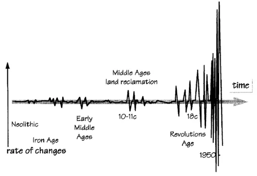
Throughout ages human impressed obvious traces of those interventions on the territory. Since Roman colonization to nowadays lands have been strongly modified in their land use for example from marshland to agricultural land, in their aspects creating roads network reticules and other landmarks like the Roman centuriation that represented the seeds for further settlement development (fig.1).

Figure 1 – Landscape structure defined by the mesh of Roman centuriation

However, while in the past, until the Second World War, changing dynamics of farming were likely to be gradual and discernible, after that time because of the conversion from a sustainable-oriented farming to a market-oriented farming, the development of residential settlements into agricultural space , and the progressive abandonment of low income rural area produced a rapid and abrupt transformation that is still leading to an ecological simplification and cultural erosion of the traditional rural landscape. In Flanders the concept of traditional landscape was introduced in 1985 by Antrop to carry out a study aimed at classifying geographical regions. Traditional landscapes have been defined as the landscapes which evolved during centuries until the fast and large scale modern changes started, with the introduction of technological power, thus corresponding to the Industrial Revolution time period. The modern impacts became really invasive after World War II with the economical boom that followed (see fig. 2). These changes deform the traditional structures, and thus

their functioning, of the existing landscapes. In some places the traditional landscape was entirely substitute with completely new landscape. The modern landscapes are mainly characterised by uniform and rational solutions. Relicts of the traditional landscape structures still exist but in form of isolated patches which are more and more difficult to recognise.

Figure 2 - Graph of magnitude and frequency of landscape evolution in Europe (Antrop 1997).

According to Antrop (1997) the traditional landscapes can be defined as those landscapes having a distinct and recognisable structure which reflects clear relations between the composing elements and having a significance for natural, cultural or aesthetical valuesand literal in their approach. Consequently such definition is referred to these landscapes with a long history, which evolved slowly and where it took centuries to form a characteristic structure reflecting a harmonious integration of abiotic, biotic and cultural elements.

I.1.2 The rural built environment

The rural built environment is the result of human action and represents one of the most important cultural element of the rural landscape. In its traditional forms it is an expression of humble culture, derived from agro-pastoral activity. The traditional artefacts are often made from local materials (wood, stone, earth, etc.) and have function of houses, stables, barns, local processing and storage of products, etc.. Technical solutions are essential, and practical to enable the farming activity and the use of all possible environmental resources. The advance of technology and modernity in building and agriculture have gradually changed the rural system by introducing campaigns works designed with the latest functional criteria,

made using materials and equipment that are often inspired by models construction or industrial production. This has prompted to production development, but has also encouraged a gradual degradation of the landscape and the architectural quality of the overall agricultural areas, and the inclusion of facilities and activities within rural areas and that increase their impact on the environment. Emilia Romagna region, located in the north-eastern pert of Italy is on of the region mostly characterized by a prevailing agricultural production vocation and were transformation dynamic intensively occurred. It has been recognised as including many interesting cases of aggregation and urban sprawl by numerous authors, including Ingersoll (2001, 2002) and Indovina et. al. (2005) and therefore assumed as area of investigation of such phenomena. The traditional farm in Emilia Romagna was organized in residential building and different rural annexes functional to agricultural activity such as stables and haylofts. The whole arranged complex of buildings was named rural court (fig.3).

Figure 3 - Rural court

In these last decades rapid transformation due not only to the introduction of new technologies in the production process but also to new agricultural polices and new economic dimension generated deep modifications in the agricultural sector and in particular in the role that agricultural activity has assumed in the production system. The abrupt conversion happened after second world war shifting from a subsistence agriculture to an industrial agriculture characterized by a high use in pesticide and mechanization and so by a

rearrangement of farm lands to allow such interventions provoked a general simplification of the rural landscape. Elements of rural landscape losing their original functionality related to rural context were quickly modified or substituted with more suitable uses for modern agricultural practices or new land use destinations. Rural built environment as component of rural landscape has been strongly affected by such dynamics. Traditional farm buildings, due to their recognised unique elements, are important within the countryside. They may have visual qualities as part of the landscape, and they may have archaeological or historical value giving an indication of previous farming practices. In many cases buildings have been restored without considering such valuable elements and contrasting the original arrangement of rural landscape. Traditional farm buildings may no longer be required for their original use. Uses other than for agricultural purposes tend to be favoured, such as residential and business uses because they provide more benefits. The intense allocation of production factors related to urban activity in the rural spaces with a high level of antropic activity deeply modified original landscape. As a consequence there is an infiltration of urban patterns within agricultural spaces developing new assets where rural and urban patterns are both existent. Such interactions provoke several negative effects such as sprawl effect of settlement and a gradual conversion of rural spaces into urban. The subtraction of agricultural lands for urban purposes is becoming more and more intense attracting attentions of several academic fields at national and international level. Since landscape is an multidisciplinary topic because of the manifold resources involved, different disciplinary groups are taking in charge of the analysis of dynamics with the common purpose of preserving and protecting the landscape heritage. On this scenario planning policies represent a key tool by means of actuating a sustainable development of landscape. It is well known that the study of landscape changes is an essential stage for the promotion of conscious decision making in land planning. Institutions in charge of planning and programming should be aware of dynamics occurred in the past in order to prevent future scenario. On this purpose the comprehension of reasons responsible for landscape transformation results to be important elements to gain a better knowledge of possible present and future rural landscape dynamics. The study of changes in the landscape is a topic widely discussed in scientific community at national and international level. The analysis of changes occurred on various components of rural landscape with the main purpose of identifying reasons related to such transformation and to forecast future scenarios of evolution, represents an important tool and indeed a prerequisite as part of the landscape planning and programming. In relation to both these objectives techniques are frequently used, for

modelling space, covering different time interval and adopting different methods depending on the specific field of analysis and resources of the landscape investigated. In particular the rural built system represents an important component of the landscape mosaic, whose type of development has a significant impact on the overall rural landscape evolution.

I.2 AIM OF THE STUDY

The specific aim of the presented study is to propose a methodology for the development of a spatial model that allows the identification of driving forces which mostly have influence on building allocation.

It is well known that the study of landscape changes is essential for conscious decision making in land planning, and analytical methodologies aimed to such study are part of a topic broadly developed by the scientific community. The review of the scientific literature carried out pointed out the importance of focusing on criteria for analysing the trends in the rural built environment and on landscape modelling techniques which can be developed for such purposes, but also a general lack of modelling methodology for the study of rural built environment changes.

There are mainly two types of transformation dynamics that have been recognised as affecting the rural built environment: the conversion of rural buildings and the increasing of building numbers. The present study decided to focus on the analysis of the latter dynamic for reason related to the concerning issues brought about by the expansion of built up areas in rural landscapes. Moreover another distinction must be done regarding the dynamic affecting the increasing of building number. Similarly to what occurs in land use change analysis, the investigations on rural building expansion can be carried out following two different approaches: the identification of the rate of expansion of rural buildings or the identification of their spatial allocation. Each of this option generates a very different outcome. In the first case the answer addresses to the question which rates the expansion are likely to progress, i.e. the quantity of expansion, and in the second case where the expansion is likely to take place. The allocation analysis is based on spatial analysis of the complex interaction between rural built system, socio economic condition and biophysical constraint locations of land use change and requires the identification of the natural and cultural landscape attributes which are considered the spatial determinants of change. Conversely, the rate or quantity of change are driven by demand for land-based commodities (Stephenne and Lambin, 2001) and in the

case of land use change models they, are often modelled using economic framework (Fisher and Sun, 2001). This means that driving forces which control the rate of changes operate at higher hierarchical levels hence that they often involve macro-economic transformation and policy changes (Lambin et al., 1999).

Understanding the spatial distribution of data generated from events that occur in space constitutes today a great challenge in many research fields because it results having direct implications in planning activities. In fact the importance of recognising driving forces that operate in the selection of land suitability for building construction represents a much more useful tool than the detection of rates. In the decision making process, actuated for planning purposes, it is fundamental to know driving forces responsible for the allocation of new built up-area in order to contrast irrational expansion of building across landscape and to prevent urban sprawl and landscape fragmentation.

Hence the design of the model involved the identification of predictive variables (related to geomorphologic, socio-economic, structural and infrastructural systems of landscape) capable of representing the driving forces responsible for landscape changes. The response variable was represented by a binomial function indicating presence or absence of buildings in a general location of the study area.

L

ITERATURE REVIEW

II. LITERATURE RIEVIEW

Scientific literature provides a wide range of studies that deal with landscape changes and provides different socio-economic or ecological approaches.

According to Antrop (2000), landscape should be considered as holistic, relativistic and dynamic. Landscape is dynamic in the sense that the nature of the composing elements changes under diverse impulse including human action. In particular, over the last century the evolving of landscape became increasingly affected by human behaviour determining abrupt changes such as in land use, species distributions, land morphologies. For this reasons, efforts from scientific communities are mostly tuned on transformation analysis. In literature there are many application examples such as Turner (1989), Li et al.(1993) and Dunning et al. (1992) that used various landscape indexes to measure landscape structure under different conditions to assess entity of change. They reveal that such studies are not sufficient to explain some research questions, there is also a need for models.

Models of landscape changes have been reviewed by Shugart and West 1980; Louks et al.1981; Weinstein and Shugart 1983; Shugart 1984; Risser et al.1984; Shugart and Seafle 1985 and Baker 1989. A variety of criteria could be used to distinguish models of landscape change. In 1987 Baker proposed an approach for the study of landscape change based on these following two criteria: (1) the level of aggregation, and (2) the use of continuous or discrete mathematics. The level of aggregation criterion refers to the level of detail with which the landscape change process is modelled. Following this approach, Baker classified landscape models into three categories: (1) whole landscape models, (2) distributional landscape models, and (3) spatial landscape models. Whole landscape models focus on the value of a variable or several variables in a particular land area. Distributional landscape models emphasize changes in the distribution of lands cover types. Spatial models, on the other hand, use the location and configuration of landscape elements in projecting change and explicitly produce maps of these changing spatial configurations. Whole landscape models describe the characteristics of a certain landscape; distributional models examine or predict changes of landscape distribution over time; and spatial models determine where the changes might occur. Markov model are probably the most commonly used distributional models. Spatial landscape models take into account the spatial configuration of the landscape phenomena and recently this approach thanks to advancement with GIS technologies found wider application in landscape modelling. Spatial model are classified in mosaic landscape model in which change in mosaic of individual subarea is modelled and element landscape

model in which change in individual landscape elements is modelled. The main difference is that in the first case the change is measured in subarea by which landscape is divided. The phenomena for example the amount of houses are taken within a equal portion in which landscape is subdivided like a mosaic shape. In this way it’s known the amount of change per subarea. The element model landscape focus on the response of individual element to the spatial configuration. Such type of model find application for the study of organism in habitat distribution model and they use grid cell or vector-based mapped organism location. Literature shows some cases in which this approach is applied for modelling individual landscape element since analogies can be existent between these two entities. Especially where biotic interaction strongly control the character of landscape element or create patches, individual organism model may be more appropriated then mosaic model.

Rural landscapes often absolve complex and competitive demands of society. For example, they are used by people to generate income (ex. agriculture, mining, and tourism), to provide a living space, and to provide quality of life (clean water, recreation, and social activities). Rural landscape has created indeed a new ecosystem and a better understanding of the ecology of the landscape and the whole complex of components is needed to provide sustainable future rural landscapes. Nichol G.E. et al. (2005)proposed a classification model braked into model domains and subdomains: socio economic, biophysical (land-use, ecology, soil and water hydrology, hydrogeology, agricultural production, environmental pollution and nutrient flow), and generic and integrative (planning support system, visualization, decision support system, risk assessment, climate change). The subdomain of land use and land cover change models have become increasingly common because of the dramatic expansion of developed area that provokes fragmentation of landscape and urban sprawl. Early models of land-cover and land-use change were essentially non-spatial (e.g., Johnson, 1977). Later models incorporated a set of explanatory variables that might themselves be spatially patterned. The probability of development at some pixel i is a function of a vector x of explanatory variables.

More complicated functions in x can contain information on state of nearby pixels, given the model attribute of cellular automata (Neumann, 1966; Wolfram, 1984; Hogeweg, 1988). The Spatially explicit land use/cover change models can be divided in three categories: simulation, estimation and a hybrid approach that includes estimated parameters with simulation. Many of the simulation models are based on a cellular automata approach. These are a class of mathematical models in which the behaviour of a system is generated by a set of deterministic or probabilistic rules that set the state of a cell based on the states of neighbouring cells.

Individual cell states are updates on the base of neighbour cell states in the previous time period. Such models have been used widely to study process of urban growth (Wu and Webster,1998; Clarke et al.,1997; White et al.,1997; White and Engelen, 1993; Batty et al., 1989). The progress made in technology using GIS technology and remote sensing have made possible the incorporation of the space-time components at different levels of resolution within the model enhancing the modeling space for the study of the territory (Sklar & Constanza 1991). As the landscape is a complex entity and the use of dynamic modeling space was an important support in decision-making in the government of the territory for those involved in planning activities (Behan 1990), other are the benefits of its implementation, in particular the possibility of conducting simulations that can be displayed on the territory of study, to relate the phenomenon being studied with the surrounding factors and their distribution in time and space (Dunnning et al.1995). A wide use of this tools is common among geographer for developing spatially explicit empirical models. Examples from literature include Mertens and Lambin (1997), Andersen (1996), LaGro and DeGloria( 1992). These focus on the aspect that deforestation whose data are acquired by means of remote sensing and represent the dependent variable are related to some explanatory variables also derived from the remotely sensed data.

In the majority of case studies, it is usual to fit a single model to the data describing land use change, then test that model and use it for projection into the future. additionally the focus in many models is the hypothesis testing and similar situation exists in ecology in relation to models of the distribution of plants and animal species, where for example a single model is developed from empirical data and use to predict distribution (Guisan and Zimmermann, 2000).

A wide range of studies is available for the modelling of urban area expansions. Referring to these an interesting approach is developed by W.F.Fagan et al., 2000. The stated hypothesis is that urbanization expansion must be considered as an ecological colonization process in which individual colonists (houses) occupy available space and influence subsequent development. From this perspective, processes of built-up area expansion are similar in many ways to the growth of plant population or the growth of animal species. Reasons that prompt to formulate such theory is mainly because urban growth have captured interested from geographers, environmental planners, and social scientist (e.g., Chapin and Weiss 1968), also developing urban growth models mostly by using neural network linked with GIS platforms, (Weisner and Cowen 1997) and heuristic optimization techniques (Densham 1991; Batty and

Densham 1996) but always lacking of an ecological approach. Hence, it is generally perceived the importance of incorporating also ecological principles into the analysis of human-dominated systems.

Another topic related to agricultural sector where literature review provides wide of contributions is agricultural land-use modelling. Agricultural land-use modelling has a long history, dating back to the agricultural location theory developed in the late 1700s. The last 10 years has seen an increasing attentions from many scientific communities perhaps because of the availability of cheaper and more powerful computer technologies, and the coming of natural resource management issues in many different fields which are often associated to the strong impact that agricultural activity has on natural environment. The need for useful models is increasingly apparent. A wide variety of methods has been developed that seek to have an impact on problem solving. Examples include spatial models of herbivore (Coughenour, 1991), crop distribution models (Carter and Jones, 1993), agricultural location models to explain deforestation patterns (Chomitz and Gray, 1996), explanatory Markov rule-based models of land-use dynamics in a watershed (Stoorvogel, 1995), and a whole array of statistical and simulation models that contain

some spatial components to study land-use and deforestation processes, (reviewed by Lambin, 1994).

Although a wide literature review that faces issues related to rural environment, changes occurred on rural built environment have never been treated as specific objective of study, except for one case reported by R.Aspinall, 2004. This illustrated a case study carried out in Montana, where rural housing change locations are uses as parameter of land use change. The design model is used to develop a series of different models reflecting drivers of change at different periods in the history of the study area.

It can be said that there is a general lack in scientific literature of models for the study of rural built environment changes, that instead represent an important component of rural landscape recently affected by strong transformation dynamics.

M

ATERIALS

&

METHODS

III. MATERIALS AND METHODS III.1STUDY AREA

To test the model developed by following the defined methodology, it is necessary to apply the model to a case study. Hence to select a study area as a target, together with a time range that are representative of dynamics under study where to carry out the calibration process. The significance of the landscape for the phenomena under study motivates the adoption of a study area located in the northern part of Italy within Emilia Romagna Region named New District of Imola (a description of the study area is reported in paragraph III.1). The time range selected for testing the model is the interval between 1975 and 2005 since such period of time is extremely meaningful for transformations occurred on rural built environment.

Figure 4 - New District of Imola.

III.1. 1 NEW DISTRICT OF IMOLA

The study area is located in the eastern part of Bologna Province within the Emilia Romagna region. The extension is approximately 787 Km2 _{with a population of 125.000 habitants and it}

is comprehensive of ten municipalities which are characterised by sharing similar geomorphologic conditions and historical past events.

The landscape is heterogenic: flat lands extending to the northern part gradually turn into hills and relieves moving toward the southern part. For each of these landscape scenarios small or medium municipalities are sprawl across the territory.

Existent municipalities find their origins in pre-existent ancient settlements and they still maintained some residuals of traditional rural activity that were developed in accordance with the type of environment. Along this heterogeneous landscape, different typologies of rural settlements are well represented, as expression of rural architecture adaption to the agricultural activity at different environments. Significant geomorphologic and landscape diversification, make possible to observe structured dynamics for all the main land use systems and have an overall depiction of rural built environment and keep trace of transformation occurred in different types of landscape.

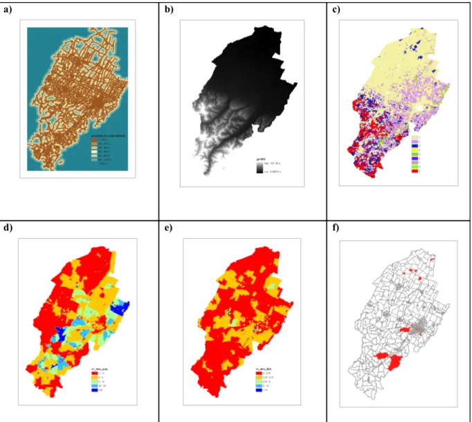
Figure 5 - Study area morphology

The elevation digital model allows to distinguish in the study area three main thresholds at 50, 300, 600 and 900 m above sea level, which respectively individuate three regions: plain area

(46% of the entire area), hill-foot area(38% of the entire area), hilly area (15% of the entire area) and low mountain (1% of the entire area) (fig.5). The most important river that crosses the area is represented by the Santerno whose valley follows a flow direction from the southwest to northwest between Apennines and foot-hill area. The landscape of the southern part of the study area is portrayed by hills that sometimes is characterized by marginal agriculture and uncultivated areas, forests.

According to a research study reported by Tassinari et al (2007), the province of Bologna, between 1976 and 2003, showed an expansion of the inhabitant urban centres and an intensification of the urban fringe starting from Bologna centre and extending along the main roads. Such expansions are particularly stressed along the most important road which is the via Emilia (fig. 7).

Others important sprawls occurred also across flat lands followings the surrounding of Santerno and Reno rivers. Also a fusion between Bologna’s urban territory and the one of the municipalities in the immediate suburbs, with the consequent formation of a compact urban area has been observed, and in particular its ultimate boundary is larger than the municipal boundaries of the main city and embraces farm fields and fringe area. The growth of towns increase along via Emilia until the city of Imola.

In the flat part that still follows the structure defined by the mesh of Roman centuriation it can be easily recognised the via Emilia, which ideally divides the study area into a northern flat and a southern hill part. The study area has been object of a classification resulting from the analysis of elevation joint to agro forestry land use suitability defined by Klingebiel and Montogomery, 1961.

III.1.2. HISTORICAL BACKGROUND

The first significant actions on the territory under study, occurred in the Roman era in particular with centurition whose form impressed the landscape and maintained over time representing a base for various subsequent transformations. Also Marinelli in the XIX century states that, over 100,000 hectares of plains of Italy, apparently among the most fertile, reveal the obvious division of the ancient land. Roads, canals and ditches follows a pre-territorial division, and a network of roads and drains that can not easily be changed (fig.6)

Figure 6 - Landscape structure defined by the mesh of Roman centuriation. The side of the mesh was set to 700 meters.

In Roman ages the capacity of modifying the landscape was very intense, resulting a strong man-made landscape. The ancient road, via Emilia, built in the 187 B.C by Marco Emilio Lepido as a connection between Rimini, on the Adriatic coast, to Piacenza, on the river Po, passing through Bologna, Imola, Faenza has always represented one of the most important route of the Pianura Padana region. This vast country, by far the largest fertile plain in the mountainous peninsula, contained potentially its best agricultural lands, and offered to Romans the opportunity to expand enormously their population and economic resources by means of massive colonisation.

Figure 7 - Via Emilia in red.

During the second century B.C. various seed dwellings grew spontaneously in strategic geographic positions such as in proximity of Lamone and Santerno rivers that became: Forum Corneli (Imola) and Favente (Faenza). During medieval times, after the fall of the Roman Empire, Romagna became part of the Byzantines domain, with the generation of a peculiar settlement systems inherited from Roman named as fundus and massa.

In that period, despite the loss of some centres, cities in Romagna continued to serve as a core for aggregations, increasing settlements. This trend is in contrast to what happened in urban centres of Lombard region, where number of settlements dropped down. An interesting dynamic in this period was the development of large properties (particularly ecclesiastical) with a consequent consolidation of funds.

Towns were built slightly before XI century and they inherited a basic structure that would have been never altered by subsequent interventions. After XI century in territories surrounding Imola the dynamics of population were attracted by the construction of churches and rural settlements scattered around the countryside. Between the middle of XIV century and the beginning of XV Imola was affected by a strong expansion of the urban perimeter

because of a wide immigration that placed the city among the twenty most populous of the peninsula. Until XIV there were not significant events that introduced changes in Romagna landscapes.

Among the XIV-XV century the introduction of the asymmetrical plow, determined a change in the form of fields, no longer square but rectangular lengthened.

During XIV-XV century the landscape is strongly characterized by a form of promiscuous crop called Piantata (arbustum gallicum) (fig.8), formerly known in Etruscan era, with the main function of drainage. These lines defined the shape and size of farms, paths and fields. The transformation of Piantata began during XVIII century with the introduction of new crops such as corn and hemp crops requiring highly exhausting new agricultural practices with great movement and transportation of soil and resettlement of hydraulic structures. Not only lines of Piantata and drains contributed in the shape of rural landscape but also trails that were built for transportation and communication uses.

Figure 8 - Piantata

The construction of a rail that privileged Bologna brought some crisis in the productivity of the Romagna plain. As rebalancing intervention some connections were created in Romagna

such as a steam tramway Bologna - Imola, which integrated the Imola area in the space of Bologna.

After the building of numerous roads made from 1859 onwards, agriculture improved its production by about 1 / 3 of grain and rice. In this system increased the viability of minor roads having a key role in the overcome of farm fragmentation. Consequently countries were continually intersected by these roads forming a reticule representative of the huge land fragmentation level of these lands. The crisis of agricultural production because of the market of Asian and American products dropped the production of wheat which represented the main product of farms.

Beet crops at the beginning of 1900 was already successfully progressing in the rotation as agricultural crop roots and renewing. The advent of beet crop cultivation affects strongly the agricultural landscape. In these lands, between the national union and the first world war, landscape assumed profiles of long chimneys with sugar beet factories almost everywhere along the railway lines and spreading through cultivated fields.

Starting from 1920 the agricultural landscape of the land reclamation changed, following the introduction of wide orchard systems in Romagna, which for many years it was always maintained in extensive and not promiscuous intensive, with consequent relocation of facilities serving such activities as cold stores etc. According to the description of a typical rural landscape in Romagna at the beginning of 1900, reported by Oliva, the intensive form of cultivation determined a rectangular geometric shape of farm fields with a range of length between 500 msq to 8000 msq. This regular shape of fields evidences the remarkable mark of mesh created during roman centuries Such traces can be easily recognized along via Emila, on the border between Bologna and Modena, and between Lugo and Imola.

The second world war ended with the destruction of cities including infrastructure and hydraulic defence systems bringing a period of general crisis and poverty.

Several actions helped to improve the situation in this period of reconstruction. The main event was the opening of the domestic fruit market. This spurred the building of utilities related to fruit and vegetable market in Romagna.

The strong productivity growth not only affected the fruit sector but also brought radical changes at social and demographic levels resulting on abrupt modification of rural landscapes structure. In particular the growing use of mechanization in agriculture caused the abandonment of traditional cultural forms no longer adequate since an obstacle to new technologies, such as the destruction of the green lattice of piantata. Since the 60s, there has been a drastic reduction in agricultural area according to the abandonment of less productive

lands and the increasing use of lands for urbanization and industrialization. Starting from a considerable fragmentation of extended land possession, those generated a rapid spread around small towns addressed preferably for building purposes.

III.2 DEVELOPMENT OF THE MODELING METHODOLOGY

The analysis of driving forces of landscape transformation dynamics represents one of the main research topic in many fields of study with the common main purpose of developing a sustainable planning activity aimed at preserving and protecting landscape resources.

Several ecological indicators have been developed in order to reflect a variety of aspects related to the ecosystem, including biological, chemical and physical, but they are not sufficient in order to understand reasons involved in changing process and to support simulation of future scenario. For such purposes more suitable analysis tools, such as statistical modeling techniques, that allows to understand driving forces and future scenario, needed to be introduced.

According to M.P. Austin (2002), three components are needed for statistical modeling: a model concerning the theory to be used or tested, a data model concerning the collection and measurement of data, and a statistical model concerning the statistical theory and methods used. In the following paragraphs are processed these steps that lead to the definition of the most suitable model for the comprehension of reasons related to built environment allocation within rural and periurban area. The model developed by following the methodology is applied to a case study to test the validity of the methodology. In particular the model has the specific aim of testing the existence of a cause-effective relationship between some possible factors affecting expansion dynamics and the increase of the built environment in term of their allocation. Hence the first step in the development of the model consists in identifying driving forces responsible for rural built environment expansion. This assumption also called hypothesis is formulated stating the existence of a cause effective relationship between selected driving forces and building allocation process.

III.2.1 THEORETIC MODEL

A different combination of factors in various parts of the territory generated favourable or less favourable conditions for the building allocation and the existence of buildings represents the

evidence of such optimum. Conversely, the absence of buildings reflects a combination of agents which is not suitable for building allocation. Presence or absence of buildings can be adopted as indicator of such driving conditions, since they represent the expression of the action of driving factors in the land suitability sorting process. The existence of correlation between site selection and hypothetical driving forces, evaluated by means of modeling techniques, provides an evidence of which driving forces are involved in the allocation dynamic and an insight on their level of influence into the process.

GIS software by means of spatial analysis tools allows to associate the concept of presence and absence with point futures and generate a point process. This is expressed by a set of distributed points in a terrain. In case of presences, points represent locations of real existing buildings, in case of absences they represent locations were buildings are not existent and so they are generated by a stochastic mechanism avoiding the overlapping with the existent built environment. The location of points is the object of study, which has the objective of understanding its generating mechanism.

The methodology proposes to identify driving forces acting upon landscape affecting rural built transformation and then test the actual existence of a causal relationship between them and the building allocations in the expansion process through a model. Therefore the recognized driving forces responsible for changes represent the hypothesis to be tested. The set up of an hypothesis to be tested through a model recalls approaches adopted for the modelling of population distribution where similarly an initial hypothesis is tested by means of empirical models. Empirical models in fact, statistically relate the geographical distribution of species or communities to their present environment.

The model that seeks to be developed is a spatial explicit model because it is by means of the spatial arrangement assumed by new buildings across the landscape that the comprehension of related driving forces is realised. In fact the building site locations is the expression of the action of driving factors in the land suitability sorting process and such condition is synthesized through a spatially explicit modeling approach. Spatial explicit models consider how elements that generate the landscape are changing in space and typically produce maps representing these dynamical patterns. For the specific case study, the outcome map represents, if compared with the actual existent building arrangement, a test for the theoretical assumption formulated.

To test the model developed according to the defined methodology, it is necessary to apply the model in a case study, hence to select a study area as a target, together with a time range that are representative of dynamics under study. The availability of spatial data regarding

building locations together with the significance of the landscape motivates the adoption of a study area located in the northern part of Italy within Emilia Romagna Region named New District of Imola (a description of the study area is reported in paragraph III.1). The time range selected for testing the model is the interval between 1975 and 2005 since such period of time is extremely meaningful for transformations occurred on rural built environment. Two different dataset are applied in modelling building expansion in periurban and rural area, hence two separate calibration processes were carried out. The identification of rural and periurban area refers to the classification adopted for the stratification of the random sampling methodology (see paragraph III.3). In this case study, periurban area is assumed as the output resulting from the spatial difference between urban area existent in 2003 and urban area in 1976 (see fig.9).

The outcome resulting from spatial intersections between sample areas - rural area and sample areas - periurban area, represented the land where spatial data were acquired on which to perform the calibration process.

III.2.2. RESPONSE VARIABLE

The issue at this stage is related to the definition of the best variable able to explicit the building expansion dynamic. Since the objective of the model is the understanding of driving forces having effect on building expansion within rural and periurban area, the dependent variable should be a factor which could explain the variation of buildings over time. In the analysis of building expansion there are two dynamics that seek to be explained: (1) the increasing rate of built up area and (2) locations taken by new buildings. Most models (see Clarke and Herold 2002; Silva and Clarke 1995, White 1993, Verburg et al. 1999), developed with the purpose of analysing the built-up area expansion, have the aim of understanding reasons related to the conversion of different types of land use/land cover and then predict future scenarios. Only few studies were carried out (Aspinall 2003) with the specific intent of focusing on transformations occurred at higher scale in rural built environment. In particular, among different aspects related to built environment transformation in rural area, it seems that there is a general lack of studies dealing with the modeling of rural building expansion. Therefore, it is a specific purpose of this work to provide a modelling methodology for the transformation analysis of building expansion. In particular as explained in the paragraph related to the aim of the study, the interest is focused on the transformation analysis of building allocations.

As previously explained a different combination of factors in various parts of the territory generated favourable or less favourable conditions for the building allocation and the existence of buildings represents the evidence of such optimum. Conversely the absence of buildings expresses a combination of agents which is not suitable for the allocation of buildings. Presence or absence of buildings can be adopted as indicator of such driving conditions and represent the response variable of the model. Sites where building take place are characterized by conditions that acting in a different way within the territory generate perhaps a different evolution of the landscape. It is important hence to set an appropriate variable able to register such existing conditions. Presence or absence of buildings at some site locations represent the expression of these driving factors interaction.

Therefore it is expected that response variable can assumes two values with a discrete distribution along the study area, to register where new edification occurred or not over time. This circumstance can be expressed by a binomial type of variable that assumes the value of 1 for the event corresponding to presence of the building and 0 for the opposite event i.e., absence of buildings.

In fact, for the correct application of the model not only new edifications must be detected and related to their driving factors, but also sites where none building allocation occurred. The expression of variation of building in a quantitative way such as variation of number of buildings or density of building per area, do not represent a suitable approach since would report information solely related to the increasing of built up area not on the distribution that new allocation assumed. It is instead by means of qualitative variable that reasons related to new presence or absence of new building allocation can be understood

GIS software by means of spatial analysis tools allows to associate the concept of presence and absence with point futures generating a point process. In case of presences, points representing buildings are indicated as 1, in case of absences points are generated by a stochastic mechanism avoiding the overlapping with the existent built environment and are indicated as 0. This is a very basic operation that allows to attach environmental information to building spatial locations labelled as points.

The assignment of presence or absence is made on the basis of a diachronic analysis carried out on the same study area. The comparison, between two time steps, allows to locate new buildings. In practice, this is performed at first by overlapping maps of the built environment, represented by polygon features, of the same territory in two different time intervals. Buildings added at the very next time step represent the new building built in favourable sites and therefore indicated as presences. To associate values that driving factors assume in building locations it is necessary to perform a spatial intersection. This operation can not be performed if new buildings, hence those labelled 1, are polygons, because such typology feature doesn’t allows to capture precisely the value of each driving factors existing in correspondence of each building location. The possibility to transform polygon into points overcome this problem.

GIS facilities that handle two-dimensional topological structures do not need a complex of vertices and line segments to define a polygon, but simply a point (a pair of coordinates) called centroid or label. In procedures for reconstruction of the topology, the software performs a research through the entire geographic database to assign to the fields LPOLY (left polygon) and RPOLY (right polygon) of the arc attribute table correct identifiers of individual

centroids. For this reason, points and polygons (or points and centroids) share the same list of attributes, which in the case of points by convention, is called Point Attribute Table and in the case of polygon they are abstract items such as centroids of the polygons, Polygonal Table of Attributes. Polygon Attribute Table of contains in any case an area and perimeter. In the Point Attribute Table, these two fields are of course for all records equal to zero. Hence it is possible to transform each polygon representing a building in its respective label point or centroid (fig.10).

In correspondence of point feature locations the response variable assumes value of presence hence labelled with 1.

Since also factors responsible for none building occurrence have to be tested in the model, random points are generated outside building polygons, preventing any overlapping with existing polygon and labelled with 0 (fig.11).

In this way, the variable assumes a binomial distribution which belongs to a type of theoretical probability distribution family and expresses the probability of occurrence of the specific event: building presence or absence.

Figure 10 - Generation of label points from building polygons.

Absence of buildings have the function of identifying factors that are not favourable for building allocations. This represents an important component for a correct application of the model. The parameterization of this variable was performed generating randomly a certain

number of points equal to the amount of new buildings. Such random points are created within sample areas avoiding any possible overlay with already existing buildings (fig. 11). Their generation required at first the rasterization of sample area and then the use of a specific tool. There are some different tools available for this purpose and in this case was adopted the Hawth’s tool.

Figure 11 - Generation of random points within sample areas.

SAMPLE AREAS

III.2.3 DATA COLLECTION: RANDOM STRATIFIED SAMPLING METHODOLOGY

In order to develop a spatial model, an important requirement is the availability of spatial data related to building locations. Mapping building spatial configuration in different time intervals considered for the analysis is essential in order to estimate variation of the built environment. Obviously such requirement involves a large quantities of spatial data referred to built environment in rural area and periurban area. These spatial information are not easily to be collected especially for time interval located in the past where more likely, maps reporting building location for geographical area, are still in paper format and so not useful to carry out spatial data elaboration in GIS environment. Digital format for such type of spatial information in the most part of Italian region became available after 2000. The digital acquisition of spatial data from paper map is extremely time consuming and so demands the application of a sampling methodology in order to extract representative sample area on which to proceed with the acquisition of building spatial locations.

At this purpose a stratified random sampling methodology, resulting from an additional study carried out in cooperation with the research group of the division of Spatial Engineering of DEIAgra (University of Bologna) for a broader research work, is proposed as a sampling data collection model. The referring methodology (see Tassinari, et. al., 2008 ) represents a fundamental step for the development of the case study. In fact, to test causal relationship between building locations and related acting driving factors it is essential to have spatial information of each new building occurred within a time interval in the study area. The supplying of such parameter, represents a critical phase in the data acquisition process. In particular, since the study focus on transformation occurred in past decades after the second war, spatial information regarding building locations at this time step results as to be the most required. Proceeding backward to seek for information represents a difficult task in data collection process. The specific case of rural built environment analysis relies on data able to provide locations of buildings in the past and in ages not far from the actuality and the conversions of spatial data for buildings distribution which are solely available in paper format into digital vector format is extremely time consuming. On the other hand this step is essential for the comparison of different land arrangements and the evaluation of changes over time. Whereupon the application of a sampling methodology represents a fundamental and compulsory tool for change studies carried out on rural built environment.

The stratified sampling methodology at the end allows to extract representative sample areas of the territory under analysis where to carry out the acquisition and processing of data avoiding to undertake this procedure for the entire study area.

The design of the proposed method for stratified random sampling goes through this following steps:

• Delineation of a suitable sampling framework

• The stratification of the study area according to some variables and criteria for setting population elements

• The extraction of representative sample areas

The stratification methodology was developed on a target study area which is the New District of Imola.

Stratification process involved the identification of variables that mostly affect the development of rural built environment directly and indirectly and on which combination define possible strata. The first stratification variable was the land use, for which 5 classes were defined (this task was carried out in collaboration of GIS department of Emilia Romagna Region).

Land capability connected to elevation were identified as based variable for the stratification because for long time new settlement sites took place and growth where environmental and morphological condition where more favourable to agricultural activities. Hence it seemed logical to aggregated these two variables generating one unique variable named as land suitability for agriculture and forestry production. This is classified in 5 possible categories of suitability to agricultural uses becoming one of the stratification variables (fig.12).

Figure 12- Agro-forestry capability classified in 5 categories:

Highest level of agricultural land-use suitability (a); flat area with vertisoil (b); foot-hill and hill area with medium level of agricultural suitability (c); lower agricultural suitability of class c (d); lowest agricultural

suitability (e).

In area sampling can be chose a sampling frame that subdivide the study area based upon physical boundaries or a lattice built with regular geometrical outline. In the case study proposed, is presented the first option and the area sampling was define according to the most recent Italian population and estate census (Istat, Italian Statistic Board, 2001). Istat provides classification of Emilia Romagna Region by dividing the area into division census polygons of different sizes based upon number of buildings (see fig. 13).

Figure 13 - Istat census polygons

There are four types of census divisions based on the level of buildings aggregation:

• populated centres (highest level of aggregation); • scatter centres (distances among houses ≤30m);

• productive centres (included in the extra urban area outside of dwellings and towns area

where there are at least 200 employed and 10 buildings);

• sprawl houses (none texture of contiguity is observed).

This type of census divisions classification approach is particularly suitable to meet the purpose of defining a sampling frame for the extraction of a representative pilot sample on which carry out studies for rural built environmental dynamics. In fact the extension of census division polygon and hence of sampling frames are sized based on number of buildings, so smaller polygon are in urban area and in its proximity, and larger polygon are in rural area where buildings have more disperse distribution.

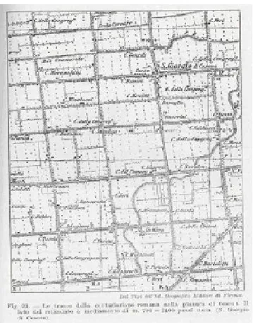
The land-use/land-cover represent another variable introduced for the stratification. The data for analysis of land-use/land-cover patterns were acquired from the most recent thematic maps available i.e., those produced by the GIS Department of Emilia-Romagna Region via photo-interpretation of panchromatic orthoimages acquired by the Quickbird satellite in 2003. Such landuse/ land-cover maps, drawn on a scale of 1:25000, present a vector-type geographical structure with a minimum mapping unit of 1.56 ha. The land-use applied as variable for the stratification process was classified in 5 classes (see fig.14):

1. settlements;

2. crop fields and mixed;

3. orchards, greenhouses, garden;

4. silvo-pastoral area, wetlands, area with no vegetation; 5. water bodies and rivers.

The intent of this classification is to suit local characteristics at the greatest level of detail, a key structure referring to the four levels of the Corine Land Cover (European Environment Agency, 2000).

Figure 14 - Land use classification.

Hence the stratification of the Istat census division is performed based upon the combination of the two stratification variables: land-use and land suitability.

The first stage of stratification process consists in identifying all census division occupied by more then 50% of urban area and then subdivide them based on the second stratification variable the land suitability according to a majority attribution criteria. Periurban area is defined as a specific stratum since this area experiences the most marked changes in land use/land cover change with particular transformation dynamics typically of urban fringe. In this case study periurban area is considered as a particular portion of territory characterized by the presence of typical urban building arrangements such as those assumed by Istat

classification however located in the rural area according to the land use classification and photo-interpretation. Visually this stratum is displayed as the result of the difference between census district polygons classified as populated centre according to Istat classification and census divisions assigned to urban according to the 2003 land- use/land-cover classification. The classification of extra-urban areas is first carried out identifying the predominant portion of land use/ land cover class in term of extent and then assigning the prevalent land suitability class relative to this. In the specific case study, the necessity of having a small number of strata and the existence of few strata generated by some combination variables, validated the hypothesis of aggregate together certain strata characterized by having the same land use/land cover but different land suitability. Twelve strata were obtained in which each strata is named from the combination of the number of the corresponding land-use/land-cover class assigned and the letter of the corresponding land suitability class. The selection of the sample area can be done using the method of permanent random number (see Carfagna, 2007). More specifically, this involved assigning to each population element in a stratum a real number between zero and one following a uniform distribution and then sorting the elements of the stratum in ascending order according to their randomly assigned number. Following this sequence, a number of elements were then selected from each stratum corresponding to the sample fraction assigned to that stratum by the proportionate allocation criterion. This methodology applied to the study area chosen as target for the calibration of the methodology generated 103 sample areas where was possible to acquire spatial data related to each single building location (see fig.15). Spatial building information within sample area in the past were detected according to a methodology (Tassinari and Torreggiani 2006) that apply a process of backward updating. Maps related to past distribution of rural built system back at 1975 and cadastre at 2005 were compared and buildings that did not yet exist at the previous time step were removed and, if necessary, added where any existing one were subsequently demolished. Spatial information regarding building locations in 1975 within sample areas were collected and mapped in digital format. Consequently, the spatial building expansion was determined performing the spatial overlay of the two maps displaying building distribution in 1975 and in 2005 within representative areas. The new edifications resulting by the difference of the two layers represented the presences of the response variable that was transformed into the value of 1 for the purpose of fitting the GLM.

Figure 15 - 103 Sample areas extracted

III.2.4 GENERATION OF DATAFRAME

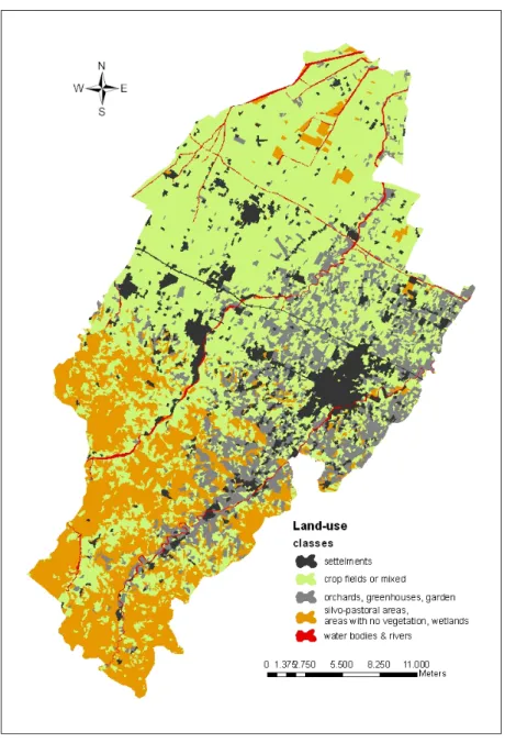
The spatial building allocation of new buildings resulting from the spatial difference between building distribution in 1975 and in 2005 within sample areas therefore recorded as 1 are labelled as points. Absence of buildings, labelled with points as well, are instead generated randomly still within the sample areas and recorded as 0. These two operations are performed for buildings located in urban and periurban area independently. It is clear that since the spatial processing to determine the allocation of new buildings can be carried out only within sample areas, it is necessary to individuate and extract within these areas, portion of rural and portion of periurban area and on these portions determine spatially the building allocation occurred from 1975-2005 (see fig 16). On the same portion, random points representing absences are generated (see fig 17). The number of random points generated must be the same as points representing new buildings detected in the spatial difference process within sample areas.

Figure 16 - Presence (new buildings) and absence (random points) of buildings on the layer resulting from the intersection of rural area and sample areas.

Figure 17 - Presence (new buildings) and absence (random points)

of buildings on the layer resulting from the intersection of rural area and sample areas.

Random points New buildings Periurban area Sample area

The attachment of variable values to points, representing presence/absence of building sites, and the consequently generation of the data frame for the calibration process of rural and periurban model, was carried out by performing an intersection in ArcMap with the Hawth’s tool which performs a point-grid overlay (see fig. 18).

Figure 18 - Hawth’s tool point intersection.

The table of contents generated by the overlay process displays for each record the pixel value that explanatory variables take in correspondence of the dropped points that own the presence or absence feature (see table 1).

Table 1 - Table of contents resulting from the intersection of points, that own presence (P) or absence (A) feature, with raster layer of explanatory variables.

P/A proximity to roads proximity to periurban proximity to urban slope building density pop. density elevation

1 502.49377441400 1215.08227539000 1237.61865234000 11.66663265230 0.78401023150 0.00000000000 543.29693603500 1 484.66482543900 1191.06042480000 1212.20874023000 11.66663265230 0.78401023150 0.00000000000 543.29693603500 1 488.36462402300 1198.85363770000 1223.93835449000 11.75392818450 0.78401023150 0.00000000000 548.17541503900 1 80.00000000000 1606.54907227000 110.67971801800 26.49568748470 0.78401023150 0.00000000000 426.59887695300 1 70.71067810060 1653.98010254000 140.89002990700 28.55367660520 0.78401023150 0.00000000000 416.22967529300 1 36.05551147460 147.05441284200 185.00000000000 11.06765747070 4.99766588211 0.16699999571 160.09582519500 1 10.00000000000 237.53947448700 587.06896972700 25.36139297490 4.99766588211 0.16699999571 180.03361511200 1 793.09521484400 1525.81945801000 1240.25195313000 11.61035633090 0.76076006889 0.00000000000 497.36206054700 … … … … 0 778.97369384800 1470.00854492000 1298.47985840000 9.28243732452 0.76076006889 0.00000000000 487.28359985400 0 31.62277603150 2410.85058594000 199.06028747600 7.62764549255 1.82184815407 0.13600000739 384.61099243200 0 20.00000000000 164.46884155300 801.63891601600 6.53141641617 4.99766588211 0.16699999571 137.52951049800 0 14.14213562010 2372.18261719000 241.29856872600 1.42608094215 1.82184815407 0.13600000739 387.39886474600 0 60.00000000000 130.86251831100 848.76379394500 5.33002614975 4.99766588211 0.16699999571 134.95545959500 0 0.00000000000 2349.06884766000 260.86395263700 9.56576442719 1.82184815407 0.13600000739 384.57385253900 0 0.00000000000 2276.92773438000 377.35925293000 15.94096374510 1.82184815407 0.13600000739 351.51116943400 0 58.30952072140 2178.46264648000 385.81082153300 17.78398132320 1.82184815407 0.13600000739 351.06872558600 0 44.72135925290 2160.02319336000 365.85516357400 19.87686538700 1.82184815407 0.13600000739 342.35061645500 0 31.62277603150 1972.23217773000 235.05319213900 24.77745628360 1.82184815407 0.13600000739 309.96017456100 0 70.71067810060 1653.87426758000 203.03939819300 23.81204986570 1.82184815407 0.13600000739 221.89361572300 [1] [1] [1] [0] [1] [0] [0] [0]