Volume 39, Issue 2
An explorative analysis of Italy banking financial stability
Matteo Foglia
Department of Economics, “G.d''Annunzio” University of Chieti-Pescara
Eliana Angelini
Department of Economics, “G.d''Annunzio” University of Chieti-Pescara
Abstract
This paper provides a quantitative measure for the financial stability of Italy banking sector. First, we construct an indicator that summarizes the information about the health of Italy's banking system, the Bank Condition Index (BCI). The index is constructed with capital adequacy, asset quality, earnings and liquidity (CAEL) indicators. The major advantage of BCI is that can be useful for initial identification of bank soundness and can be helpful to identify the principal areas of weakness. Furthermore, we apply AR model to evaluate the predictive power of the BCI on GDP growth. The results identify that the BCI is an important predictor of real economic activity. Finally, we study the relationship between the BCI and systemic risk measures (DCoVaR, SRISK, DCI), finding that an increase of systemic risk implies a reduction of bank-financial stability.
Citation: Matteo Foglia and Eliana Angelini, (2019) ''An explorative analysis of Italy banking financial stability'', Economics Bulletin, Volume 39, Issue 2, pages 1294-1308
Contact: Matteo Foglia - [email protected], Eliana Angelini - [email protected].
Submitted: January 25, 2019. Published: May 31, 2019.
1
Introduction
The global financial crisis (2007-2009) has highlighted the importance of financial sta-bility to reduce the risk spread, namely systemic risk. In order to evaluate it, is essential to measure the contribution of each financial institution to the overall risk of the system, as well as their links with the real economy. Given the bank-based nature of financing to non-financial corporations and households in the euro area, is necessary to monitor the health of these banks, basic prerequisite for economic and financial stability (Gramlich and Oet 2011). In fact, bank stability is influenced by the prevailing conditions in the financial market and the real economy and its control is crucial to economic expansion (Minsky 1991; Calderon et al. 2004).
Our goal is to offer quantitative metrics of the financial stability for the Italy banking system. The banking sector is the most important segment of the Italy financial system and as such need attention. Therefore, we choose to study this country because 1) it has a very significant number of banks and 2) the Italy distress period caused high levels of non-performing loans. This suggests that the Italy banking system could be more dangerous respect to other Europe banking system. To inspect the fragility of this banking system represents an important challenge.
To this, we build an indicator that summarizes the information about the health of banks, the Bank Condition Index (BCI). The BCI is constructed using a wide range of variables that are commonly used to characterize the condition of the banking sector. As a rough measure of individual banks’ health, we use CAEL1
(Capital adequacy, Asset quality, Earnings, and Liquidity) type ratings. Indeed, this approach is a measure of banks’ soundness (Chiaramonte et al. 2015).
Composite indices are progressively used for assessment of the stability of the finan-cial system2
. For example, the Financial Stress Index (Illing and Liu 2003; Hanschel and Monnin 2005; Oet et al. 2011), the Financial Condition Index (Hatzius et al. 2010; Gumata et al. 2012), the CISS index (Holl´o et al. 2012), the Financial stability index (
ˇ
Cih´ak et al. 2013). However, the episodes of systemic banking crises stimulated various studies that use bank-level data. Our work is closely related to a recent strand of litera-ture which attempts to estimate financial stability indicators by CAMELS (Arena 2008; Mishra et al. 2013; Bode 2016) methodology.
To calculate the index, we apply a simple average analysis that can be seen as repre-senting the fundamental forces influencing the banking system and can be used as a set of weight for the BCI3
. The major advantage of BCI is that can be useful for initial identi-fication of bank soundness and can be helpful to identify the principal areas of weakness. Also, in order to evaluate the overall degree of tightness of conditions in the banking sector, we test the relationship between BCI and the growth rate of real GDP. We expect that the growth of GDP has a positive effect on the banking system (BCI), as well as the contrary. Our findings confirm this link. Finally, we assess the relationship between our stability index and the market-based systemic risk measures, to highlight the peculiarity
1
Policy makers and regulators use financial indicators based on the CAMELS rating for ranking individual banks by their financial soundness and risk level. A large of financial stability literature rely on the fundamental assumptions of CAMELS, which accentuate the importance of this method (Popovska 2014).
2
A comprehensive survey on prediction methods is also given in Demyanyk and Hasan (2010).
3
The weight attributed to each variable in the final index is debated point. We give an equal weight of 25 percent to each 4 categories, but one could argue that some variables are more relevant to stress than others.
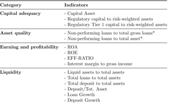
Table I: Banking Soundness Indicators
Category Indicators
Capital adequacy - Capital Asset
- Regulatory capital to risk-weighted assets - Regulatory Tier 1 capital to risk-weighted assets Asset quality - Non-performing loans to total gross loans*
- Non-performing loans to total asset* Earning and profitability - ROA
- ROE
- EFF-RATIO
- Interest margin to gross income
Liquidity - Liquid assets to total assets
- Total loans to total assets - Total deposit to total assets - Deposit/Tot. Asset
- Loan Growth - Deposit Growth
Notes: (*) indicates the variable to which the sign has been changed.
in terms of shock response of the Italian banking system. For this purpose, we estimate the contributions of major Italy banks to systemic risk (at the aggregate level) based on famous three approaches: ∆CoVaR, SRISK and the Dynamic Causation Index (DCI). In this case, we expect an inverse relation, namely an increase of systemic risk implies a decrease of stability and viceversa. Results show that risk-taking plays an important role in the dynamics of financial stability.
This research offers several contributions. First, the construction of this index allows policymakers and banking stakeholders to investigate the sources of risk in the financial system, thus allowing for better monitoring of its degree of stability. The identification of the main areas of weakness should facilitate the understanding of risk accumulation process and therefore greater control over systemic risk. Moreover, unlike other works, the index produced is easy to interpret, allowing to describe the evolution of banking health conditions over time.
Secondly, this research is a pioneer in the study of the effects of systemic risk on composite indicators of a CAMELS nature. In general, an increase in systemic risk implies a less stable and therefore riskier financial system. However, our results show that an overly resilient financial system can induce more risks. Banks are induced to take greater financial risks in quiet and safe times.
2
Composite banking condition index
2.1
Data and Methodology
The index is based on similar methodologies used in the literature on financial stability and financial stress. The aggregate micro-prudential indicators are based on the CAEL, which includes different groups of indicators that reflect the health of banks and represent the dimensions of the banking system (Mishra et al. 2013). Table I lists all variables included in BCI across all of its 4 categories. The indicators are: i) capital adequacy, ii) assets quality, iii) earnings and profitability, and iv) liquidity.
ad-dress expected or unexpected losses. Low level of this ratio indicates a potential banking crisis. According to the Basel Committee, aggregate risk-based ratios are the most indi-cators of capital adequacy. Asset quality measures the credit risk of banks. The rate of non-performing loans to total loans is a proxy of the level of credit risk and captures the amount of loans for which the bank expects that it will have difficulty to collect. Prof-itability indicators measure the efficiency of deposit takers using their capital and total assets (ROE and ROA). Liquidity affects the ability of the banking system to withstand shocks.
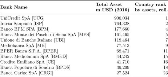
To build the index we use the first 11 top Italian listed bank firms in term of total asset and capitalization, according to Bankscope Country rank. Table II lists all banks included. All data have been taken from Bloomberg.
Table II: Bank sample
Bank Name Total Asset
m USD (2016)
Country rank by assets, roll.
UniCredit SpA [UCG] 906,034 1
Intesa Sanpaolo [ISP] 764,328 2
Banco BPM SPA [BPM] 177,660 4
Banca Monte dei Paschi di Siena SpA [MPS] 161,465 5
Unione di Banche Italiane [UBI] 118,464 7
Mediobanca SpA [MB] 77,513 9
BPER Banca S.P.A. [BPER] 68,471 11
Banca Mediolanum SpA [BMED] 44,242 15
Credito Emiliano SpA [CE] 41,710 16
Banca Popolare di Sondrio [BPDS] 39,209 18
Banca Carige SpA [CRGI] 27,524 23
Source: Bankscope (Status: Active Banks; World Region/Country: Italy (IT); Listed banks)
The calculation of BCI is realized for the period from 2002Q1 to 2017Q2. According to other works (Petrovska and Mihajlovska 2013), the sign is changed (multiplied by “-1”) for some variables (see “*” Table I) that have a negative effect on bank conditions, to ensure that all variables affect the index in the same direction. This adjustment ensures that increase of all individual indicators means an improvement in banking stability and decrease means deterioration. To construct the index, first, we have been transformed the variables into normal standardized variables in order to have the same variance,
Zt =
xt− µ
σ (1)
where Zt is the value of indicator x during period t, µ represents the mean and σ is the
standard deviation. Second, all indicators used within one category is then converted into a single index by average (size weighted):
BCIt= n
X
i=1
wiZt (2)
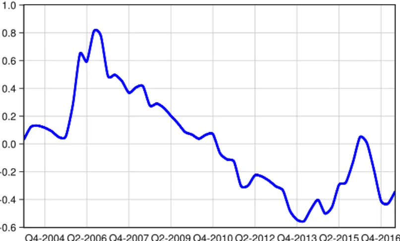
Figure 1: Bank Condition Index -0.6 -0.4 -0.2 0.0 0.2 0.4 0.6 0.8 1.0 Q4-2004 Q2-2006 Q4-2007 Q2-2009 Q4-2010 Q2-2012 Q4-2013 Q2-2015 Q4-2016 BCI
Notes: BCI (zero mean and unit variance standardize) 2-quarter moving average.
2.2
The Bank Condition Index
Figure 1 presents the aggregate BCI computed for Italy since the first quarter of 2002. A higher value represents an improvement in the banking surrounding (more resilient system) while a lower value (close to -1) represents a more vulnerability banking system. The indicator captures the main financial events occurred in recently periods showing the three-turbulence affected Italy. The index decreased significantly during the global financial crisis (2007-2009), again during the sovereign debt crisis (2010-2012) and anew at the end of 2014 (the consequence of the sovereign debt crisis). The pre-crisis period is characterised by a strong increase of credit flow to the private and non-financial sector and then good banking performance, largely thanks to the deregulation of financial markets and the convergence of interest rates at the time of the introduction of the euro.
The health of the banking system tightened in the wake of the financial crisis after the collapse of Lehman Brothers (end 2007). The financial crisis affected the capital adequacy as well as the liquidity of the banking system, pushing them to a minimum level. Since the spring of 2010, the increase in sovereign risks has been associated with a worsening of the financing conditions on E-mid markets and an increase in lending rates to households and non-financial corporation (Neri, 2013).
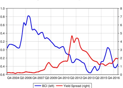
Generally speaking the transmission of shocks from the sovereign spread to bank overdrafts takes place through two channels. Specifically, the direct exposure of banks to the public sector, and the link between sovereign ratings and bank ratings (“diabolical loop”, Shambaugh 2012). This is exactly what happened in Italy, where the sovereign risks have been reflected in the profitability of banks (Figure 2).
Albertazzi et al. (2014) show that an increase of 100 basis points of the spread is associated with an increase of one quarter of the value adjustments on loans and a reduction of 4% of the interest margin and 2% for other revenues. For this reason, during the period between December 2011 and February 2012, the ECB carried out several measures of refinancing operations (LTRO, OMT, VLTRO), for the purpose of reducing the propagation of risks. The massive liquidity inflow resulted in a considerable increase
Figure 2: BCI and Spread -0.6 -0.4 -0.2 0.0 0.2 0.4 0.6 0.8 1.0 0 1 2 3 4 5 6 7 8 Q4-2004 Q2-2006 Q4-2007 Q2-2009 Q4-2010 Q2-2012 Q4-2013 Q2-2015 Q4-2016 BCI (left) Yield Spread (right)
Notes: The blue line (left side) is the BCI; red line (right side) is the Italy-German Bond Yield Spread.
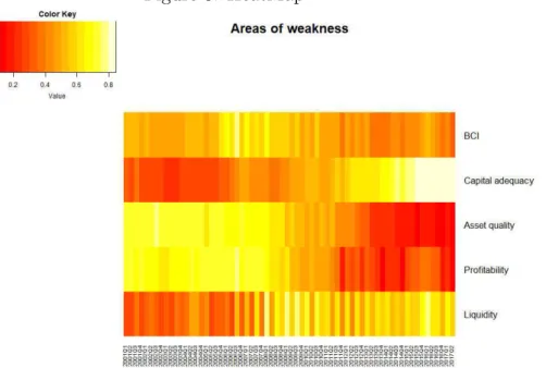
in liquidity and capital adequacy (see Heatmap, Figure 3), restoring the index to higher values. Moreover, in March 2015 the ECB implemented new measure, Expanded Asset Purchase Programme (QE), to facilitate access to the credit market and to refinance the banks (the last peak of the index). However, the difficult credit conditions were reflected in the low ability to generate income, which is an important factor of vulnerability for the Italian banking industry.
The long weakness of the economy has had a heavy impact on the profitability of the Italian banking system (Albertazzi et al. 2016). Figure 3 shows that the current levels (2017q2) of profitable are much lower than the pre-crisis (2004-07) levels, mainly due to the sharp drop in interest margin and the increase in credit adjustments. The reduction in costs and efficiency gains achieved by intermediaries in recent years have allowed the industry as a whole to contain losses but not to produce profits. Also, the severe recession has caused a sharp deterioration in the quality of credit in banks’ balances. Between 2008 and 2014, impaired loans of the entire banking system increased from 131 to 350 billion of euros (Bank of Italy 2015) and their impact on the total of loans rose from 12 to 18 percentage points. The deterioration, mainly concerned corporate loans, was spread among the economic sectors and between the geographical areas of the country, involving banks of all size classes.
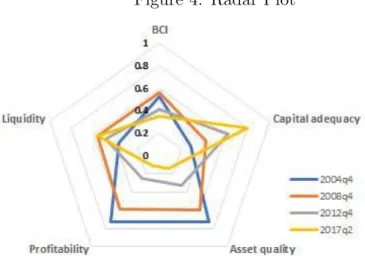
Figure 4 shows the evolution of each four categories that component the BCI. The blue line refers to 2004q4, the red line refers to Global financial crisis periods (2008q4), grey to the sovereign debt crisis (2012q4) and finally, the yellow line refers to the recent period (2017q2). Points drawn near the board indicate high health banking system (resilience), while points near the center indicate a high degree of vulnerability. As shown in the red line, in the fourth quarter of 2008, liquidity and capital adequacy index categories were at very low levels indicating the presence of vulnerability. Over the years since the crisis, as indicated by the blue line, the banks’ capital and liquidity positions have improved, unlike other aggregated indices. A series of actions carried out in the last years have contributed to increasing capital and liquidity, such as the new regulatory capital requirements (Basel 3) and the stress tests of the European Central Bank. The financial
Figure 3: HeatMap
Notes: The Heatmap provides, by assigning a colour, the evolution of each individual components of BCI, showing the areas of weakness. Us-ing exponential transformation [1/(1 + exp(−Zt))] the sub-indexes are
mapped into the (0,1) interval in order to allow for a straightforward comparison of each category over time. Values near to 0 (red) indicate the vulnerabilities in the banking sector, while values near to 1 (yellow) indicate that the banking system is safe.
crisis and sovereign debt crisis have transformed the composition of the balance sheet of the banking system. In particular, at pre-crisis periods the banking system had a high level of quality asset. As a consequence of the crisis, the balance sheet composition is opposite, with a lower level of profitable and high value of non-performing loans.
In conclusion, the BCI has deteriorated over time. During the analysed period, the index plunged to the low level in 2009q2, when the negative effects of the global economic and financial crisis on both the domestic economy were most evident, in 2011q4 when the sovereign debt crisis has burst, and finally in 2014q4 when the negative effect of the sovereign debt crisis (higher level of NPLs) on the domestic financial system was most evi-dent. The drop and increase of the index value were largely affected by: weak performance of profitability, and degradation of asset-quality. The increase of non-performing loans has the major contributed to make the system much more vulnerable. The continued uncertainty about the resolution of the stocks of NPLs and low profitability has reduced the ability of banks to enhance resilience, with several implications for financial stability in Italy. The weakness of the economic cycle and lower operating efficiency of European intermediaries will continue to exert pressure on banks’ profitability, as has been the case in the last decade (Albertazzi et al. 2016). Return to pre-crisis profitability levels is ham-pered by low interest rates that squeeze unit margins. Additional profitability pressures regard the new accounting standard on financial instruments (IFRS 9), which introduces a valuation approach based on expected loss rather than on actual realized losses.
Figure 4: Radar Plot
Notes: Using exponential transformation [1/(1 + exp(−Zt))] the
sub-indexes are mapped into the (0,1) interval in order to allow for a straight-forward comparison of each category over time.
3
The relationship between BCI and real economy
In this section, we study the empirical relationship between BCI and the growth rate of real GDP. Generally speaking, the growth of GDP is expected have a positive effect on banking system (BCI), through credit growth and asset quality, leading changes in profitability and soundness (Monnin and Jokipii, 2010; Creel et al. 2015). Hence, BCI growth is expected to be positively correlated with GDP growth. Figure 5 shows that behavioural of GDP with the BCI.
Figure 5: BCI and GDP
-0.6 -0.4 -0.2 0.0 0.2 0.4 0.6 0.8 1.0 370,000 380,000 390,000 400,000 410,000 420,000 430,000 440,000 450,000 Q4-2004 Q2-2006 Q4-2007 Q2-2009 Q4-2010 Q2-2012 Q4-2013 Q2-2015 Q4-2016 BCI (left) GDP (right)
Notes: The blue line (left side) is the BCI; red line (right side) is the GDP.
In order to provide a valuation of which values of BCI are most likely to be associated with economic growth, we apply the Granger causality test. Table III suggests that is the BCI that implies a GDP.
Table III: Pairwise Granger Causality Tests
Null Hypothesis: F-Statistic p-value
BCI does not Granger Cause GDP 4.96 0.010 GDP does not Granger Cause BCI 1.26 0.290
Also, as in Gumata et al. (2012)4
, we evaluate if BCI has greater ability to explain and predict GDP growth, applying the following equation:
(yt− yt−4) = β0+ p X i=0 βi(yt−i− yt−i−4) + q X i=0 γi∆xt−i+ εt (3)
where yt is the standardized real GDP, xt is the BCI, and the εt is the error term.
The lag (p, q) is chosen using the AIC criterion. Table IV shows the results of the autoregression model (AR).
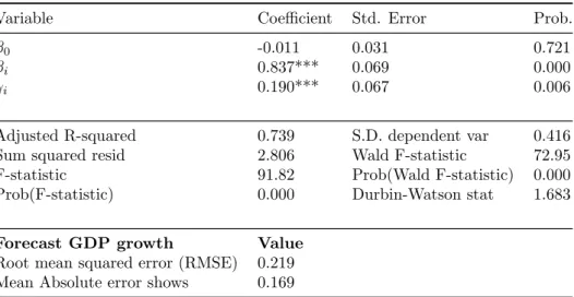
Table IV: AR model results
Variable Coefficient Std. Error Prob.
β0 -0.011 0.031 0.721
βi 0.837*** 0.069 0.000
γi 0.190*** 0.067 0.006
Adjusted R-squared 0.739 S.D. dependent var 0.416
Sum squared resid 2.806 Wald F-statistic 72.95
F-statistic 91.82 Prob(Wald F-statistic) 0.000
Prob(F-statistic) 0.000 Durbin-Watson stat 1.683
Forecast GDP growth Value
Root mean squared error (RMSE) 0.219 Mean Absolute error shows 0.169
(*) denotes statistical significance at 10%, (**) denotes statistical significance at 5%, (***) denotes statistical significance at 1%. We perform diagnostic tests for residuals using the Ljung-Box portmanteau, Lagrange Multiplier tests and Jarque-Bera test. Results indicate the absence of serial correlation and heteroskedasticity, with error normally distributed.
The AR model is stable, indeed the sum of the coefficients is less than 1. The coeffi-cient of the BCI is positive and significant, implying that the higher level of the index is associated with a higher level of GDP, as expected. The results show that the banking conditions indices help in explaining the near term GDP growth. Furthermore, there is no serial autocorrelation as provide by Durbin-Watson test (1.7), LM test (Prob.F = 0.19) rejects the hypothesis of serial correlation and the Breusch-Pagan-Godfrey test (Prob.F = 0.12) indicates the absence of heteroskedasticity, with error normally distributed ac-cording to Jarque-Bera test (3.04).
We perform an in-sample static forecast from 2008q1 to 2017q2 in order to asses the predictive power. The results, which are presented in Table IV, suggest that the BCI provides a higher predictive power of GDP growth. Focusing on the Root mean squared
4
There are many papers that use a similar approach to study the relationship between the business cycle and financial condition index (see Petrovska and Mihajlovska 2013; Darraq-Paris et al. 2014).
error (RMSE) we can see the very low level of error, as well as the Mean Absolute error shows (0.17). This implies that the BCI is an important prediction of future GDP growth, namely the co-movements of banking variables carry-out information on the dynamics of GDP growth.
4
Relationship between BCI and Systemic risk
Now we analyse the relationship between our “balance-sheet fundamental” index and the systemic risk. To this, we compute three different measures proposed in the litera-ture. We estimate the CoVaR (∆CoVaR) as proposed by Acharya et al. (2012), and by Adrian and Brunnermeier (2016) respectively. We apply the SRISK measure, proposed by Brownlees and Engle (2016). Finally, we estimate the Dynamic Causation Index (DCI, Billio et al. 2012) to study the evolution of the interconnection level between banks. A higher level of DCI suggests that the system is highly interconnected, then lower level indicates the contrary.
CoVaR measures the system loss conditional on each institution being in distress, while the SRISK measures each institution’s loss when the financial system is in distress. CoVaR expresses the “value at risk” of the financial system conditioned by a specific event that affects a specific financial firm. “Co” of VaR express the concept of co-movement, trying to capture the spillovers effects between financial institutions (Di Clemente 2018). Instead, the ∆CoVaR, expressing the contribution to the systemic risk of a specific in-stitution, is given by the difference between the CoV aRi of firm i when the firm j is
distressed and the CoV aRi evaluated when the institution j is on a median situation.
Finally, the SRISK measures the expected capital loss of institution conditional upon the occurrence of a crisis affecting the entire financial system. The institution with the highest expected capital loss, will contribute more to the systemic crisis. This implies that this company should be considered more systemically risky.
There are many papers that apply these measures to evaluate the systemic risk. Gen-erally speaking, the studies can be divided into two context approaches: a comparative analysis that examines more than one country (Engle et al. (2014) for financial sector firms in the European Union; Bierth et al. (2015) for international insurances), a single national financial system study. For example, Chang et al. (2017) and Lin et al. (2016) for Taiwan financial industry, Kleinow et al. (2017a; 2017b) for U.S. financial institutions and Latin American, Pellegrini et al. (2017) for the UK market. However, a limited num-ber of papers have been examining the systemic risk measures in Italy banking system. The empirical literature still lacks a specific study on Italy. Borri et al. (2014) is the only work, to our knowledge, that applies CoVaR and ∆CoVaR to the Italian banking context for the period 2000-2011. They find that the size is the main predictor of systemic risk.
4.1
Estimation Procedure
Once we have calculated the aggregate condition of the Italian banking system, sug-gesting that the system is in a less than optimal condition, we want to explore the effect of systemic risk in banking stability. Therefore, we want to study how the systemic risk affects the stability and which are the verse: soundness banking sector implies a low level of systemic risk or high level of systemic risk implies vulnerability. Hence, in the follow-ing section, we try to highlight these relationships by computfollow-ing a Vector Autoregressive model (VAR). Thanks to this method, we can study the dynamics of the relationship
between our stability measure and systemic risk measures for assessing the impact of innovations on these variables. A simple univariate VAR model of p order is written as:
Yt = α + A1Yt−1+ A2Yt−2+ ... + ApYt−p+ εt (4)
where Ytis a vector of time series variables (BCI, log SRISK, log ∆CoV aR, log DCI),
α is the vector of intercepts, Ai(i = 1, 2, ..., p) is the n × n coefficient matrices, while εt
is an n × 1 vector of unobservable i.i.d. zero mean error term.
However, to compute these measures of systemic risk, we need to add more data. In particular, we collect data on equity returns and market capitalization. To estimate time-varying ∆CoVaR we include a set of state variables to capture the information and the market sentiment at each period, following Borri et al. (2014). Our variables are: the VStoxx, representing the option implied volatility for Europe market, ii) the short-term spread, as a difference between 3-month Euribor and 3-month Italy bond yield, iii) the change in the 3-month Italy bond yield, iii) the slope curve, as a difference between the 3-month and 10-years Italy bond yield, and finally, iv) the change in the credit spread between corporate bonds (IBOXX Corporate Index) and the 10-years Italy bond yield. The sample size is 3410 observation for each bank, start from 2 January 2004 to 30 June 2017. All data are taken from Bloomberg.
4.2
Estimation Results
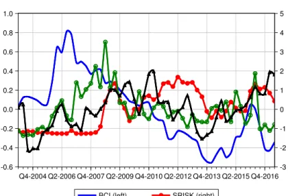
Figure 6 shows the systemic risk measures5
at aggregate level (i.e. size weighted) and BCI. All measure seems to have a similar behavioural, according to different crisis that affected the Italy banking system. The graph displays a clear positive relationship between these indexes, i.e. each measure evaluates each bank’s systemic risk contribution in a very similar way. However, these patterns are not equally strong over time.
Concentrating on ∆CoVaR, the 2008 year shows a high level of risk due to the Lehman Brothers’ bankrupt and then to the financial crisis turbulence that affects the all financial market. After, the plot shows two other peaks: the first at the beginning of the debt crisis (2010), while the second at the beginning of 2016 during the NPLs problem (crisis effects). The SRISK shows a different pattern. Low level (close to zero) on the pre-crisis period, high and persist after. The evolution follows clearly the phases of the sovereign debt crisis. The double-deep-recession (W) has had a strong impact on the balance sheets of Italian banks. The crisis has had two different phases. In the first, the Italian banking system was able to withstand the 2008 recession, caused by the collapse of subprime mortgages. In fact, Italian banks were hardly exposed. The second phase began in the second half of 2011 with the Italian sovereign debt crisis. With the new recession, the ability of borrowers to repay their debt has declined, resulting in a further increase in the rate of new impaired loans and a further increase in their size. Like the other measures show, the last peak refers to the “NPLs-issue”.
5
Figure 6: BCI and Systemic risk measures -0.6 -0.4 -0.2 0.0 0.2 0.4 0.6 0.8 1.0 -3 -2 -1 0 1 2 3 4 5 Q4-2004 Q2-2006 Q4-2007 Q2-2009 Q4-2010 Q2-2012 Q4-2013 Q2-2015 Q4-2016 BCI (left) SRISK (right)
DCoVaR (right) DCI (right)
Notes: BCI (left-side) and systemic risk measures (zero mean and unit variance standardize) on right-side.
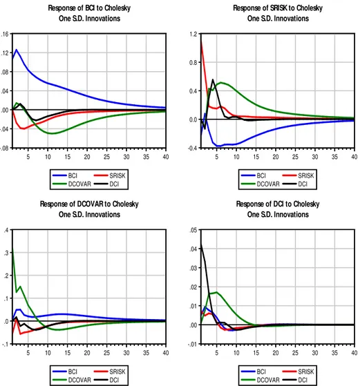
Figure 7 exhibits the impulse response (IRs) between the systemic risk measures (SRISK, ∆CoVaR and DCI) and the BCI. We focus on the relationships between our sta-bility measure and risk measures without investigating the relationships between them6
. The IRs are estimated for a horizon of 10 years (40 quarters).
A positive shock of the SRISK causes an immediate response of the contracting BCI (top-left panel); conversely, a shock of the BCI implies a reduction of the SRISK after 2 periods (top-right panel). As far as ∆CoVaR is concerned, it can be noted that an increase in systemic risk translates into a negative response of the stability of the financial system for a long time as well as an increase in interconnection (DCI) has a negative impact on the BCI but for short period. However, a positive shock of the BCI could cause an increase of the ∆CoVaR (down-left panel), as well as of the DCI (down-right panel). This controversial result could highlight a very important relationship. If it is true that an increase in systemic risk implies a less stable and therefore riskier financial system, the opposite is not true. A financial system that is too resilient can induce greater risks (i.e. the so-called risk-taking channel) for two reasons: (i) banks are induced to take greater financial risks in quiet and “safe” times; (ii) banks believe of the bailout (“too big to fail” effect). Moreover, the Italian banks, in response to the crisis, have been forced to reduce the leverage driven by the need to increase their capital ratios. Although the deleveraging process is positive for the solvency of individual banks, it may accentuate instability in financial markets. The mass sale of assets brings down the price. This implies that a possible decrease in leverage could increase the possibility of joint failure of several institutions (Papanikolaou and Wolff 2014).
6
The lag is chosen using the classic criteria information such as the Akaike Information Criteria (AIC), the Schwarz Bayesian Criteria (BIC), and the Hannan-Quinn Criteria (HQC). According to these, the appropriate numbers of lags is 2.
Figure 7: Impulse Response -.08 -.04 .00 .04 .08 .12 .16 5 10 15 20 25 30 35 40 BCI SRISK DCOVAR DCI
Response of BCI to Cholesky One S.D. Innovations -0.4 0.0 0.4 0.8 1.2 5 10 15 20 25 30 35 40 BCI SRISK DCOVAR DCI
Response of SRISK to Cholesky One S.D. Innovations -.1 .0 .1 .2 .3 .4 5 10 15 20 25 30 35 40 BCI SRISK DCOVAR DCI
Response of DCOVAR to Cholesky One S.D. Innovations -.01 .00 .01 .02 .03 .04 .05 5 10 15 20 25 30 35 40 BCI SRISK DCOVAR DCI
Response of DCI to Cholesky One S.D. Innovations
5
Concluding Remarks
This paper analyses the Italian banking sector under a “financial stability” perspective. Our goal is to make quantitative metrics of financial stability. To this purpose, first, we build an indicator that summarizes the information about bank’ health. Second, we evaluate the resilience of the financial system at systemic risk shocks.
The Bank Condition Index is based on four parameters under the CAEL criterion. The indicator shows the movement of banking health, capturing the main financial events occurred in the past 16 years. The index decreased significantly during the global financial crisis (2007-2009), again during the sovereign debt crisis (2010-2012) and anew at the end of 2014 (the consequence of the sovereign debt crisis). The vulnerability evidenced in this period has reflects the increase of non-performing loans as well as a decrease in banks’ profit. In the last years, anyway, we observe a significant improvement of capital adequacy and liquidity of the banks, which has come as a consequence of the new regulatory capital requirements (Basel 3) and the stress tests of the European Central Bank. Stability in the banking sector is a necessary condition for maintaining financial stability. As a consequence, the deterioration of the banking soundness indicator may have a negative influence on the real sector. For this purpose, we have analysed the relationship between the index and the growth of GDP. Our results show a good predictive power of BCI to GDP growth.
Moreover, we study how a systemic risk shock can affect financial stability, i.e. we compute 3 different kinds of systemic risk measures and we apply a VAR model. The findings confirm our expectation suggesting that an increase in systemic risk cause a decrease in bank-financial stability.
An improvement path would be to analyse the impact of each aggregate indicator on the real economy, to obtain the optimal level of each indicator (optimal composition). It is possible that the optimum level found is distorted by the composition of the indicator itself.
References
Acharya, V., Engle, R., and Richardson, M. (2012) “Capital shortfall: A new approach to ranking and regulating systemic risks” The American Economic Review 102, 59-64. Adrian, T., and Brunnermeier, M. K. (2016) “CoVaR” The American Economic Review
106, 1705-1741.
Albertazzi, U., Ropele, T., Sene, G., Signoretti, F. M. (2014) “The impact of the sovereign debt crisis on the activity of Italian banks” Journal of Banking & Finance 46, 387-402. Albertazzi, U., Notarpietro, A., and Siviero, S. (2016). “An inquiry into the determinants of the profitability of Italian banks” Bank of Italy, Economic Research and International Relations Area working paper number 364
Arena, M. (2008) “Bank failures and bank fundamentals: A comparative analysis of Latin America and East Asia during the nineties using bank-level data” Journal of Banking & Finance 32, 299-310.
Bank of Italy (2015) “Financial Stability Report” n. 2, November
Bierth, C., Irresberger, F., and Weiß, G. N. (2015) “Systemic risk of insurers around the globe” Journal of Banking & Finance 55, 232-245.
Billio, M., Getmansky, M., Lo, A. W., and Pelizzon, L. (2012) “Econometric measures of connectedness and systemic risk in the finance and insurance sectors” Journal of financial economics 104, 535-559.
Bode, A. (2016) “Banking soundness index approach at the level of individual banks” Bank of Albania, Economic Review H2.
Borri, N., Caccavaio, M., Giorgio, G. D., and Sorrentino, A. M. (2014) “Systemic risk in the Italian banking industry” Economic Notes 43, 21-38.
Brownlees, C., and Engle, R. F. (2016) “SRISK: A conditional capital shortfall measure of systemic risk” The Review of Financial Studies 30, 48-79.
Calderon, C., Duncan, R., and Schmidt-Hebbel, K. (2004) “The role of credibility in the cyclical properties of macroeconomic policies: Evidence for emerging markets” Review of World Economics 140, 613-633
Chiaramonte, L., Poli, F., and Oriani, M. E. (2015) “Are cooperative banks a lever for promoting bank stability? Evidence from the recent financial crisis in OECD countries” European Financial Management 21, 491-523.
ˇ
Cih´ak , M., Demirguc-Kunt, A., Feyen, E., Levine, R. (2013) “Financial development in 205 economies 1960 to 2010” NBER working paper number 18946
Chang, C. W., Li, X., Lin, E. M., and Yu, M. T. (2017) “Systemic risk, interconnectedness, and non-core activities in Taiwan insurance industry” International Review of Economics & Finance 55, 273-284
Claessens, S., Kose, M. A.,Terrones, M. E. (2010) “Financial cycles: what? how? When?”, NBER International Seminar on Macroeconomics, University of Chicago Press 303-343. Creel, J., Hubert, P., Labondance, F. (2015) “Financial stability and economic
perfor-mance” Economic Modelling 48, 25-40.
Di Clemente, A. (2018) “Estimating the Marginal Contribution to Systemic Risk by A CoVaR-model Based on Copula Functions and Extreme Value Theory” Economic Notes 47, 69-112.
Demyanyk, Y. and I. Hasan (2010) “Financial crises and bank failures: A review of pre-diction methods” Omega 38, 315-324.
Darracq Paries, M., Maurin, L., and Moccero, D. (2014). “Financial conditions index and credit supply shocks for the euro area” ECB working paper number 1644
Engle, R., Jondeau, E., and Rockinger, M. (2014) “Systemic risk in Europe” Review of Finance 19, 145-190.
Gramlich, D., and Oet, M. V. (2011) “The structural fragility of financial systems: Analysis and modeling implications for early warning systems” The Journal of Risk Finance 12, 270-290.
Gumata, N., Ndou, E., and Klein, N. (2012). “A Financial Conditions Index for South Africa” IMF working paper number 12/196
Hanschel, E. and Monnin, P. (2005) “Measuring and forecasting stress in the banking sector: evidence from Switzerland” BIS Papers chapters 22, 431-49.
Hatzius, J., Hooper, P., Mishkin, F. S., Schoenholtz, K. L., and Watson, M. W. (2010) “Financial conditions indexes: A fresh look after the financial crisis” NBER working paper number w16150
Holl´o, D., Kremer, M., Duca, M. L. (2012). “Ciss-a composite indicator of systemic stress in the financial system” ECB working paper number 1426
Illing, M. and Liu, Y. (2003). “An index of financial stress for Canada” Bank of Canada. Kleinow, J., Moreira, F., Strobl, S., and V¨ah¨amaa, S. (2017a) “Measuring systemic risk:
A comparison of alternative market-based approaches” Finance Research Letters 21, 40-46.
Kleinow, J., Horsch, A., and Garcia-Molina, M. (2017b). “Factors driving systemic risk of banks in Latin America” Journal of Economics and Finance 41, 211-234.
Lin, E. M., Sun, E. W., and Yu, M. T. (2016) “Systemic risk, financial markets, and performance of financial institutions” Annals of Operations Research 262, 579-603. Minsky, H. (1991) The Financial Instability Hypothesis: A Clarification, in: The Risk of
Economic Crisis by M. Feldstein, ed., University of Chicago Press: Chicago, 158-70 Mishra, R. N., Majumdar, S., Bhandia, D. (2013) “Banking stability- a precursor to
finan-cial stability” Reserve Bank of India working paper number 01/2013
Monnin, P., Jokipii T. (2010). “The impact of banking sector stability on the real economy” SNB working paper number 5
Neri, S. (2013). “The impact of the sovereign debt crisis on bank lending rates in the euro area”, Questioni di Economia e Finanza, Bank of Italy, Economic Research and International Relations Area working paper number 170
Oet, M. V., Eiben, R., Bianco, T. , Gramlich, D., Ong S.J. (2011). “The Financial Stress Index:Identification of Systemic Risk Conditions” Federal Reserve Bank of Cleveland working paper, 11-30, November.
Papanikolaou, N. I., and Wolff, C. C. (2014) “The role of on-and off-balance-sheet leverage of banks in the late 2000s crisis” Journal of Financial Stability 14, 3-22.
Pellegrini, C. B., Meoli, M., and Urga, G. (2017) “Money market funds, shadow banking and systemic risk in United Kingdom” Finance Research Letters 21, 163-171.
Petrovska, M., and Mihajlovska, E. M. (2013). “Measures of financial stability in Macedo-nia” Journal of central banking Theory and practice 2, 85-110.
Popovska, J. (2014) “Modeling financial stability: the case of the banking sector in Mace-donia” Journal of Applied Economics and Business 2, 68-91.
Shambaugh J. (2012) “The Euro’s Three Crises” Brookings Papers on Economic Activity 2012, 157-230.