Seismic analysis of offshore wind turbines on bottom fixed support structuree: coupled and uncoupled analyis

SCUOLA DI DOTTORATO

UNIVERSITÀ DEGLI STUDI MEDITERRANEA DI REGGIO CALABRIA

DIPARTIMENTO DI INGEGNERIA CIVILE, DELL’ENERGIA, DELL’AMBIENTE E DEI MATERIALI

(DICEAM)

DOTTORATO DI RICERCA IN

INGEGNERIA MARITTIMA, DEI MATERIALI E DELLE STRUTTURE

S.S.D.ICAR/08 XXVII CICLO

S

EISMIC ANALYSIS OF OFFSHORE WIND TURBINES ON

BOTTOM FIXED SUPPORT STRUCTURES

:

COUPLED AND

UNCOUPLED ANALYSIS

PHD STUDENT:

Natale Alati

SUPERVISORS:

Ing. Giuseppe Failla

Prof. Felice Arena

HEAD OF THE DOCTORAL SCHOOL

Prof. Felice Arena

NATALEALATI

S

EISMIC ANALYSIS OF OFFSHORE WIND TURBINES ON

BOTTOM FIXED SUPPORT STRUCTURES

:

COUPLED AND

Il Collegio dei docenti del Dottorato di Ricerca in Ingegneria Marittima, dei Materiali e delle Strutture è composto da:

Felice Arena (coordinatore) Giuseppe Barbaro Guido Benassai Paolo Boccotti Vittoria Bonazinga Michele Buonsanti Salvatore Caddemi Enzo D’Amore Giuseppe Failla Vincenzo Fiamma Pasquale Filianoti Enrico Foti Paolo Fuschi Sofia Giuffrè Carlos Guedes Soares Giovanni Leonardi Antonina Pirrotta Aurora Angela Pisano Alessandra Romolo Adolfo Santini Francesco Scopelliti Pol D. Spanos Alba Sofi

Abstract

Offshore wind energy is one of the most import renewable energy resources worldwide. In the last year, the growth of energy demand and the great potential of wind resources in the sea have encouraged the realization of offshore wind turbines (OWTs).

The present thesis investigates the seismic response of a horizontal axis wind turbine on two bottom-fixed support structures for transitional water depths (30-60 m), a tripod and a jacket, both resting on pile foundations. Fully-coupled, non-linear time-domain simulations on full system models are carried out with the software BLADED© under combined wind-wave-earthquake loadings, for different load cases, considering fixed and flexible foundation models. A comparison with some typical design load cases given by international guidelines is implemented.

Although fully-coupled non-linear time domain simulations provide the “exact” numerical solutions, they involve some significant disadvantages: (i) a dedicated software package is needed, capable of accounting for inherent interactions between aerodynamic, hydrodynamic and seismic responses; (ii) computational costs are significant, almost prohibitive when several analyses have to be implemented for different environmental states and system parameters, as in the early stages of design.

For these reasons, in this thesis, the results of uncoupled analysis, obtained as linear superposition of separate wind, wave and earthquake responses with an additional damping referred to as aerodynamic damping, will be compared with fully-coupled non-linear time domain simulations. Important conclusions will be drawn on the reliability of uncoupled analyses for seismic assessment of OWTs.

Contents

Introduction _______________________________________________ 1

1.

Offshore wind turbines ___________________________________ 5

1.1. Introduction ... 5

1.2. Aerodynamics ... 9

1.3. Hydrodynamics ... 20

1.4. Structural model ... 22

2.

Seismic analysis of wind turbines: general aspects ____________ 27

2.2. Seismic assessment of HAWTs ... 28

2.3. International standards and Certification guidelines ... 31

2.3.1. IEC 61400-3 Standards………..31

2.3.2. GL 2012 Guidelines………...33

2.3.3. DNV-OS-J101 Standards………...34

3.1. Introduction ... 37

3.2. Support structures ... 40

3.3. Load cases ... 44

3.4. Response to a single earthquake record... 48

3.4.1. Response for fixed foundation model………49

3.4.1. Response for flexible foundation model………52

3.5. Response to an earthquake set ... 52

3.5.1. Stress resultant and tower top acceleration demands for fixed foundation model………53

3.5.2. Stress resultant and tower top acceleration demands for flexible foundation model………58

3.6. Comparison with the IEC 61400-3 load cases ... 60

3.7. Conclusion ... 63

4.

Uncoupled analysis of offshore wind turbines ________________ 67

4.2. Structural models and environmental loads ... 73

4.4. Numerical results ... 77 4.5. Conclusion ... 105

References ______________________________________________ 107

APPENDIX A ___________________________________________ 117

APPENDIX B ___________________________________________ 119

APPENDIX C ____________________________________________ 123

APPENDIX D ____________________________________________ 127

Publications _____________________________________________ 137

Figures

Figure 0.1: Components of offshore wind turbines ... 2

Figure 1.1: Global cumulative installed wind capacity until 2014 (Source WWEA). ... 6

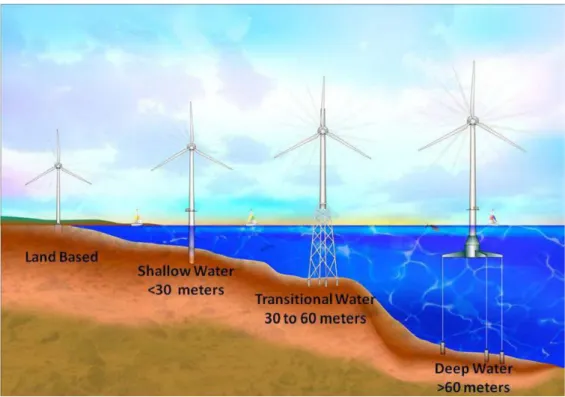
Figure 1.2: Natural progression of substructure design for different water depth... 8

Figure 1.3: Actual disk model of wind turbine. ... 10

Figure 1.4: Power and thrust coefficient CP and CT as a function of axial induction factor for an ideal horizontal axis wind turbine. ... 13

Figure 1.5: Stream tube model of flow behind rotating wind turbine blade... 14

Figure 1.6: Stream tube model of flow behind rotating wind turbine blade... 15

Figure 1.7: Blade element model. ... 17

Figure 1.8: Blade geometry for analysis of horizontal axis wind turbine. ... 17

Figure 1.9: Slender vertical members with hydrodynamic loads. ... 21

Figure 2.1: Simplified and full-system models of fixed offshore wind turbines. ... 29

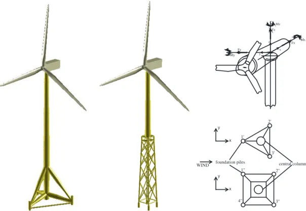
Figure 3.1: Tripod and jacket support structures, pile foundations and positive stress resultants. ... 41

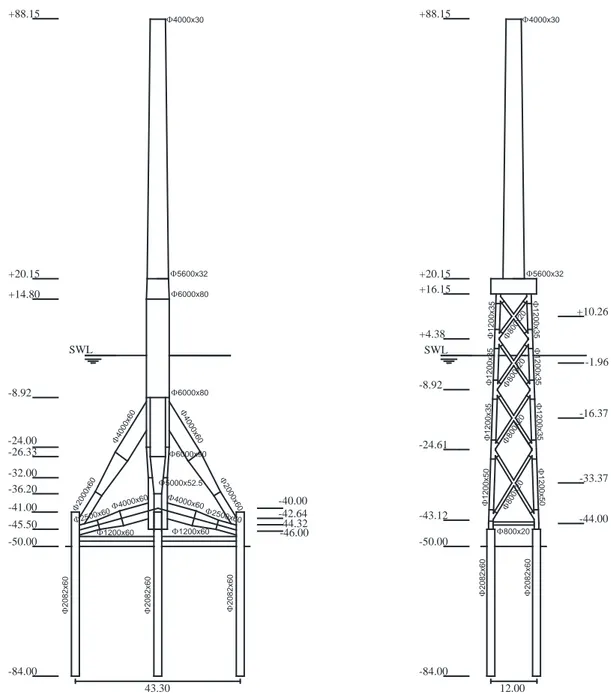
Figure 3.2: Geometry of Tripod and Jacket (dimensions of structural members in mm; heights and depths in m). ... 42

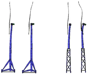
Figure 3.3: First and second FA support structure modes of Tripod and Jacket. ... 44

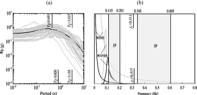
Figure 3.4: (a) 5% damped SRSS acceleration response spectrum for the earthquake set (black line: mean value); (b) wind and wave power spectral densities (black line: load cases LC1/LC2; grey line: load case LC3). ... 48

Figure 3.5: Tripod: tower top deflection and maxima acceleration profiles in x and y direction for fixed and flexible FMs. ... 50

Figure 3.6: Jacket: tower top deflection and maxima acceleration profiles in x and y direction for fixed and flexible FMs. ... 51

Figure 3.7: Tripod: stress resultant and tower top acceleration demands under the earthquake set for fixed and flexible FMs. ... 56

Figure 3.8: Jacket: stress resultant and tower top acceleration demands under the earthquake set for fixed and flexible FMs. ... 57

Figure 3.9: Tripod and Jacket pile maxima lateral deflections in x and y directions. ... 59

Figure 4.1: Sign convention for stress resultant at the tower base. ... 75

Figure 4.3 a)-b): Tripod: Errors (4.5)-(4.6) for various potential aerodynamic damping values, under Cape Mendocino earthquake. ... 82 Figure 4.4 a)-b): Tripod: Errors (4.5)-(4.6) for various potential aerodynamic damping values, under Imperial Valley earthquake. ... 84 Figure 4.5 a)-b): Tripod: Errors (4.5)-(4.6) for various potential aerodynamic damping values, under Northridge earthquake. ... 86 Figure 4.6: Tripod: Errors (4.5) for 4% aerodynamic damping, under Cape Mendocino earthquake. ... 87 Figure 4.7: Tripod: Errors (4.5) for 4% aerodynamic damping, under Imperial Valley earthquake. ... 88 Figure 4.8: Tripod: Errors (4.5) for 4% aerodynamic damping, under Northridge earthquake. ... 89 Figure 4.9: Tripod: mean demands along the tower Hs = 5m – Tp = 9.5s. ... 90 Figure 4.10: Tripod: mean demands along the tower for Hs = 6m – Tp = 11s. ... 91 Figure 4.11 a)-b): Jacket: Errors (4.5)-(4.6) for various potential aerodynamic damping values, under Cape Mendocino earthquake. ... 95 Figure 4.12 a)-b): Jacket: Errors (4.5)-(4.6) for various potential aerodynamic damping values, under Imperial Valley earthquake. ... 97 Figure 4.13 a)-b): Jacket: Errors (4.5)-(4.6) for various potential aerodynamic damping values, under Northridge earthquake. ... 99 Figure 4.14: Jacket: Errors (4.5) for 4% aerodynamic damping, under Cape Mendocino earthquake. ... 100 Figure 4.15: Jacket: Errors (4.5) for 4% aerodynamic damping, under Imperial Valley earthquake. ... 101 Figure 4.16: Jacket: Errors (4.5) for 4% aerodynamic damping, under Northridge earthquake. ... 102 Figure 4.17: Jacket: mean demands along the tower Hs = 5m – Tp = 9.5s. ... 103 Figure 4.18: Jacket: mean demands along the tower Hs = 6m – Tp = 11s. ... 104

Introduction

The demand for energy will continue to increase in the coming years and offshore wind energy shows great potential to become a key player in renewable energy future. The wind flow offshore is more stable and the average wind velocity is higher than onshore, in particular in the North Sea where the first installation of offshore wind turbines began in 1990s. In 2002 and 2003, the first large, utility-scale offshore farms were commissioned. The Horns Rev and Nysted wind farms, both in Denmark, were the first farms built with capacities exceeding 100 MW. As of the end of 2008, there was over 1000 MW of installed wind capacity, most of it in Europe.

Offshore wind energy has several promising attributes. These include:  greater area available for siting large projects;

 proximity to cities and other load centers;

 general higher wind speeds compared with onshore locations;  lower intrinsic turbulence intensities;

 lower wind shear.

There are some differences than onshore wind turbines, as;

 higher project costs due to a necessity for specialized installation and service vessels and equipment and more expensive support structures;

 more difficult working conditions;

 more difficult and expensive installaion procedures;

 decreased availability due to limited accessibility for maintenance;  necessity for special corrosion prevention measures.

According to the IEC 2009, the offshore wind turbine is defined as “a wind turbine with a support structure which is subject to the hydrodynamic loading”. This type of turbine consists of the following components (see Figure 0.1):

 Rotor-nacelle assembly (RNA): is the part of a wind turbine that capture the kinetic energy of the wind and converts its to electrical power. It includes:

- rotor: part of a wind turbine consisting of the blades and hub;

- nacelle assembly: part of wind turbine consisting of all components above the tower that are not part of the rotor. This includes the drive train, bed plate, yaw system, and the nacelle enclosure.

2 Introduction

 Support structure: this consists of the tower, substructure and foundation:

- tower: part of the support structure which connects the substructure to the rotor-nacelle assembly;

- substructure: part of the support structure which extends upwards from the seabed and connects the foundation to the tower;

- foundation: part of the support structure which transfers the loads acting on the structure into the seabed.

Figure 0.1: Components of offshore wind turbines

This dissertation is focused on the seismic response of offshore wind turbines on two different fixed support structures for transitional water depths.

Chapter 1 contains the general aspects that influence the design of offshore wind turbines, illustrates the basis for the estimation of aerodynamic and hydrodynamic loads and the structural model adopted for the simulation of the full system.

Introduction 3

Chapter 2 provides an introduction about the seismic demand of horizontal axis wind turbines and analyses the aspects of international standard and certification guidelines for the load combinations with seismic excitations.

Chapter 3 shows the results of fully-coupled non-linear time domain simulations of offshore wind turbines on two bottom fixed support structures ( tripod and jacket) for different foundation models: fixed and flexible.

Chapter 4 presents the result of uncoupled analysis for the support structures tripod and jacket with fixed foundation model.

1. Offshore wind turbines

The design of offshore wind turbines is one of the most fascinating challenges in renewable energy. Meeting the objective of increasing power production with reduced installation and maintenance costs requires a multi-disciplinary approach, bringing together the expertise in different fields of engineering. The purpose of this chapter is to offer a broad perspective on some crucial aspects of offshore wind turbines design, discussing the basis of aerodynamic and hydrodynamic loads and presenting the approaches adapted to performing integrated design load calculations for offshore wind turbines.

1.1. Introduction

In the last decades offshore wind energy has attracted a growing interest from scientists and engineers worldwide. After the first offshore wind farm, built in 1991 in relatively shallow waters (2-5 m) off the coast of Denmark at Vindeby, many others have been constructed, especially in the North and Baltic Seas, and new ones are being developed in Europe, United States, China and other countries [1]. Offshore wind energy still represents a small quote part of the total wind energy in the world, about 7 GW out of 393 GW at the half of 2015, but has an enormous potential (see Figure 1.1). The European Wind Energy Association (EWEA), for instance, estimates that offshore wind energy production in Europe will increase from the 6.5 GW at the end of 2013 to 150 GW in 2030, meeting approximately 14% of Europe's electricity demand [2-3]. Offshore sites offer indeed some considerable advantages over onshore sites, as:

 in the sea, the wind blows more stronger and constant respect land wind; as consequence the turbines are more efficient since they can produce more electricity and they can maintain higher levels of electricity generation for longer periods;

6 Chapter 1

 with the offshore wind farms the noise and the visual imapct are significantly reduced, allowing for the designers of the wind turbines to produce larger wind turbines with longer blades that can effectively produce more electricity;

 vast expanses of uninterrupted open sea are available and the installations will not occupy land, interfering with other land uses.

However, due to several issues as more difficult and specialised installation procedures, more expensive support structures, more difficult environmental and working conditions, offshore wind energy may still be more expensive not only than onshore wind energy, but also than conventional power resources. Therefore, closing this gap has become a key step a future sustainable exploitation of offshore wind energy potential.

Figure 1.1: Global cumulative installed wind capacity until 2014 (Source WWEA).

Wind energy converters have a very long history, that in Europe traces back to the Middle Ages (for more information on the historical development, see Manwell [4]). Nowadays an offshore wind turbine is a complex ensemble of different components and subsystems: rotor, nacelle with powertrain, control and safety systems [5], and a support structure generally composed of a tower mounted on either a bottom-fixed substructure or a floating device moored to the seabed. Three-bladed, upwind rotors with horizontal axis are the conventional design solution in the industry, although alternative options (two blades, downwind rotor position or vertical axis) are under study. In the twenty-three years since the Vindeby offshore wind farm was built off the coast of Denmark, turbine size has

Offshore wind turbines 7

increased from 450 kW to 3-5 MW and even larger turbines, with rated power up to 10 MW, are being tested to be released in a near future [1].

Most of the existing offshore wind farms are in shallow waters, generally less than 20 m deep. At these sites wind turbines are mounted on monopiles driven into the seabed or resting on concrete gravity bases [6]. As the water depth increases, however, monopile solutions may require too large diameters to counteract the overturning moment and, for this reason, are not generally considered as economically feasible in waters deeper than 30 m. In transitional water depths, i.e. between 30 m and 60 m, wind turbines mounted on space multi-footing substructures such as tripods and jackets are presently considered as a best option [7]. Tripods and jackets have been used at the Alpha Ventus wind farm (Germany) in approximately 30 m of water, and jackets at the Beatrice wind farm (UK) in nearly 45 m of water, for 5-MW turbines. For waters deeper than 60 m, however, current research is investigating wind turbines on floating devices as the most economically sustainable option [8-11]. Configurations under study are generally classified based on the primary physical principles adopted to achieve static stability: the spar-buoy (or ballast stabilised floater), whose stability is provided by a ballast lowering the centre of gravity below the centre of buoyancy; the tension leg platform (TLP) (or mooring stabilised floater), where stability is achieved through mooring lines kept under tension by excess buoyancy in the platform; the barge (or buoyancy stabilised floater), where stability is achieved through the waterplane area. The spar-buoy and barge are generally moored by catenary lines, but the spar-buoy may be moored also by taut lines. Hybrid concepts using features from the three classes, such as semisubmersible floaters, are also a possibility [9]. The technical feasibility of multi-megawatt floating wind turbines has been already demonstrated by three prototypes, Hywind in the North Sea (2.3-MW turbine on a spar-buoy), WindFloat in the Atlantic (2-MW turbine on a semisubmersible floater) and Fukushima-FORWARD Phase 1 in Japan (2-MW turbine on a semisubmersible floater) [3, 12-13]. This natural progression is illustrated in Figure 1.2.

Several other prototypes are under development and, at this stage, the current effort in industry and research is primarily focused on designing economic floating systems which can compete with bottom-fixed offshore turbines in terms of cost of energy. This has become a crucial goal in the perspective of moving wind turbines further offshore, with the purpose of minimising visual impact and harnessing the large resources available; it has been estimated, for instance, that only the wind resource potential at 5 to 50 nautical miles

8 Chapter 1

off the U.S. coast could provide the total electrical generating capacity currently installed in the U.S. (more than 900 GW) [14]. Several other prototypes are under development and, at this stage, the current effort in industry and research is primarily focused on designing economic floating systems which can compete with bottom-fixed offshore turbines in terms of cost of energy.

Figure 1.2: Natural progression of substructure design for different water depth.

In the last years, a number of international Standards and Guidelines have been released for design and assessment of offshore wind turbines [15-17]. In the meanwhile, numerical modelling has progressed toward more sophisticated descriptions of structural components, mechanical and electrical subsystems of modern offshore wind turbines, along with an appropriate treatment of the incident wind and wave fields. Existing numerical models rely on modal representation, multi-body, finite element (FE) concepts, sometimes combined in mixed approaches, and involve system motion equations to be solved by fully-coupled non-linear time domain integration, to account for inherent interactions between aerodynamic and hydrodynamic responses. In fact, while aerodynamic loads on the rotor are to be derived from aeroelastic models, considering the complex interaction between air flow and rotor blades, the influence of control systems and support structure dynamics, the latter affects the calculation of the hydrodynamic loads. Hence, although in some cases and

Offshore wind turbines 9

especially in the early stages of design, simplified analyses are implemented with responses to wind and wave loads computed separately and next superposed [18-19], only fully-integrated time-domain simulations are currently recommended as the basis of final, detailed wind turbine design calculations, due to the role played by system non-linearities inherent to rotor aerodynamics, hydrodynamics, and control systems [20-22].

For either existing solutions in shallow-transitional waters or future projects in deeper waters, the objective of an efficient and cost-effective design poses engineering challenges and numerical modelling complexities, which can be solved only by an integrated approach combining the expertise in diverse fields such as, among others, aerodynamics, hydrodynamics, structural and foundation engineering; also, vibration control and health monitoring play an important role, in view of ensuring a reliable and continuous power production for sustainable investments [23-24].

1.2. Aerodynamics

Aerodynamic is the base of any theoretical and experimental study on wind turbines. Since the early days of the wind industry, the Blade Element Momentum (BEM) theory has been awarded particular favour as a robust and computationally inexpensive tool to model the rotor aerodynamics and calculate aerodynamic loads. This method was developed from helicopter aerodynamics and due to its convenience and reliability has remained the most widely-used method for calculating the aerodynamic forces on wind turbines. BEM theory couples the momentum flow theory and the blade element theory.

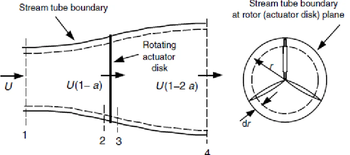
The momentum flow theory was introduced by Betz in 1926; the turbine is represented by a uniform “actuator disk” which creates a discontinuity of pressure in the stream tube of air flowing through it. The assumption of this model are:

 homogeneous, incompressible, steady state fluid;  no frictional drag;

 an infinite number of blades;

 uniform thrust over the disc or rotor area;  a non-rotating wake;

 the static pressure far upstream and far downstream of the rotor is equal to the undisturbed ambient static pressure.

10 Chapter 1

Figure 1.3: Actual disk model of wind turbine.

The analysis assumes a control volume, in which the control volume boundaries are the surface of a stream tube and two cross-sections of the stream tube (see Figure 1.3). Applying the conservation of linear momentum to the control volume enclosing the whole system, one can find the net force on the contents of the control volume. That force is equal and opposite to the thrust, T, which is the force of the wind on the wind turbine. From the conservation of linear momentum for a one-dimensional, incompressible, time-invariant flow, the thrust is equal and opposite to the rate of change of momentum of the air stream:

(

)

(

)

1 1 4 4

T =U ρAU −U ρAU (1.1)

where ρ is the air density, A is the cross-sectional area, U is the air velocity, and the subscripts indicate values at numbered cross-sections in Figure 1.3.

For steady state flow, the thrust can be expressed as follow:

(

)

m is the mass flow rate.

The thrust is positive so the velocity behind the rotor, U4, is less than the free stream velocity U1. Since no work is done on either side of the rotor, the Bernoulli function can be used upstream and downstream of the disc:

Offshore wind turbines 11 2 2 1 1 2 2 1 1 2 2 p + ρU = p + ρU (1.3) 2 2 3 3 4 4 1 1 2 2 p + ρU = p + ρU (1.4)

The pressure far upstream and far downstream of the stream tube are equal (p1=p4) and the velocity across the disc remains the same (U2=U3).

The thrust can also be expressed as the net forces on each side of the actuator disc:

(

)

2 2 3

T = A p − p (1.5)

If one solves for (p2 - p3) using equations (1.3) and (1.4) and substitutes that in equations (1.5), one obtains:

(

)

Equating the thrust value from equations (1.2) and (1.6) and recognizing that the mass flow rate is also ρA2U2, one obtains:

1 4

2

2

U U

U = + (1.7)

Thus, the wind velocity at the rotor plane, using the simple model, is the average of the upstream and downstream wind speeds.

If one defines the axial induction factor a, as the fractional decrease in the wind velocity between the free stream and the rotor plane, then

1 2 1 U U a U − = _(1.8)

(

)

12 Chapter 1

and

(

)

4 1 1 2

U =U − a (1.10)

The quantity U1a is often referred to as the induced velocity at the rotor, in which case the velocity of the wind at the rotor is a combination of the free stream velocity and the induced

wind velocity. As the axial induction factor increases from 0, the wind speed behind the rotor slows more and more. If a = 1/2, the wind has slowed to zero velocity behind the rotor and the simple theory is no longer applicable.

The power P, extracted by the wind, is equal to the thrust times the velocity at the disc:

(

)

(

)(

)

2 1 4 2 2 2 1 4 1 4

1 1

2 2

P= ρA U −U U = ρA U U +U U −U (1.11)

Substituting for U2 and U4 from equations (1.9) and (1.10) gives:

(

)

where the control volume area at the rotor, A2, is replaced by A, the rotor area, and the free stream velocity U1 is replaced by U.

The performance of the wind rotor is usually characterized by its power coefficient, Cp: 2 3 4 (1 ) 1 2 P P C a a U A ρ = = − _(1.13)

that represents the fraction of the power in the wind that is extracted by the rotor.

The maximum CP is determined by taking the derivate of the power coefficient (equation (1.13)) with respect to a and setting it equal to zero, yielding a = 1/3. Thus:

,max 16 / 27 0.5926

P

Offshore wind turbines 13

when a=1/3. For this case, the flow through the disc corresponds to a stream tube with an upstream cross-sectional area of 2/3 the disc area that expands to twice the disc area downstream. This result indicates that, if an ideal rotor were designed and operated such that the wind speed at the rotor were 2/3 of the free stream wind speed, then it would be operating at the point of maximum power production. Furthermore, given the basic laws of physics, this is the maximum power possible.

From equations (1.6), (1.9) and (1.10), the axial thrust on the disc is:

(

)

Similarly to the power, the thrust on a wind turbine can be characterized by a non-dimensional thrust coefficient:

2 4 (1 ) 1 2 T T C a a U A ρ = = − _(1.16)

CT has a maximum of 1.0 when a = 0.5 and the downstream velocity is zero. At maximum power output (a =1/3), CT has a value of 8/9. A graph of the power and thrust coefficients for an ideal Betz turbine and the non-dimensionalized downstream wind speed are illustrated in Figure 1.4.

Figure 1.4: Power and thrust coefficient CP and CT as a function of axial induction factor for an ideal horizontal axis wind turbine.

14 Chapter 1

The Betz limit, CP,max = 16/27, is the maximum theoretically possible rotor power coefficient. In practice, three effects lead to a decrease in the maximum achievable power coefficient:

 rotation of the wake behind the rotor;

 finite number of blades and associated tip losses;  non-zero aerodynamic drag.

The first correction take into account the rotation that the rotor imparts to the flow; in the case of a rotating wind turbine rotor, the flow behind the rotor rotates in the opposite direction to the rotor, in reaction to the torque exerted by the flow on the rotor. An annular stream tube model of this flow, illustrating the rotation of the wake, is shown in Figure 1.5.

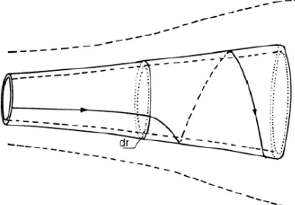
Figure 1.5: Stream tube model of flow behind rotating wind turbine blade.

The generation of rotational kinetic energy in the wake results in less energy extraction by the rotor than would be expected without wake rotation. In general, the extra kinetic energy in the wind turbine wake will be higher if the generated torque is higher. Thus, as will be shown here, slow-running wind turbines (with a low rotational speed and a high torque) experience more wake rotation losses than high-speed wind machines with low torque. Figure 1.6 gives a schematic of the parameters involved in this analysis. Subscripts denote values at the cross-sections identified by numbers. If it is assumed that the angular velocity imparted to the flowstream, ω, is small compared to the angular velocity, Ω, of the wind turbine rotor, then it can also be assumed that the pressure in the far wake is equal to the pressure in the free stream. The analysis that follows is based on the use of an annular stream tube with a radius r and a thickness dr, resulting in a cross-sectional area equal to 2πrdr (see Figure 1.6). The pressure, wake rotation, and induction factors are all assumed to be functions of radius.

Offshore wind turbines 15

If one uses a control volume that moves with the angular velocity of the blades, the energy equation can be applied in the sections before and after the blades to derive an expression for the pressure difference across the blades (see Glauert, 1935 for the derivation). Note that across the flow disc, the angular velocity of the air relative to the blade increases from Ω to Ω+ω, while the axial component of the velocity remains constant.

Figure 1.6: Stream tube model of flow behind rotating wind turbine blade.

The resulting thrust force on an annular element, dT, is:

(

)

An angular induction factor, a’, is defined as:

'

2

a =ω Ω (1.18)

The expression for the thrust becomes:

(

)

' ' 1 2 2

4 1 2

2

dT = a +a ρΩ r πrdr (1.19)

Following the previous linear moment analysis, the thrust force on an annular cross-section is:

16 Chapter 1

(

)

4 1 2

2

dT = a −a ρU πrdr (1.20)

Equating the two equations for the thrust force, it is possible to define a local speed ratio λr:

(

)

(

)

The local speed ratio is defined as the ratio of the speed at some intermediate radius to the wind speed.

Next, one can derive an expression for the torque on the rotor by applying the conservation of angular momentum. For this situation, the torque exerted on the rotor, Q, must equal the change in angular momentum of the wake. On an incremental annular area element gives:

( )( ) (

)( )( )

(

)

The blade element theory is used to calculate the aerodynamic forces on the blade as functions of lift and drag coefficients and angle of attack. As shown in Figure 1.7, the blade is assumed to be divided into N sections with the following assumptions:

 there is no aerodynamic interaction between the elements (no radial flow);

 the forces on the blades are determined solely by the lift and drag characteristics of the airfoil shapes of the blades.

The lift and drag forces are perpendicular and parallel to a relative wind velocity that is the vector sum of the wind velocity at the rotor, U(1-a), and the velocity due to the rotation of the blade. This rotational component is the vector sum of the blade section velocity, Ωr, and the induced angular velocity at the blades from conservation of angular momentum, ωr/2, or

(

)

(

)

/ 2 1

r ω r r a

Offshore wind turbines 17

Figure 1.7: Blade element model.

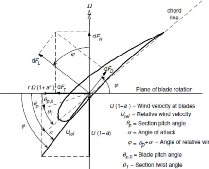
The relationships of the various forces, angles, and velocities at the blade, looking down from the blade tip, are shown in Figure 1.8.

Here, θp is the section pitch angle, which is the angle between the chord line and the plane of rotation; θp,0 is the blade pitch angle at the tip; θT is the blade twist angle; a is the angle of attack (the angle between the chord line and the relative wind); ϕ is the angle of relative wind; dFL is the incremental lift force; dFD is the incremental drag force; dFN is the incremental force normal to the plane of rotation (this contributes to thrust); and dFT is the incremental force tangential to the circle swept by the rotor. This is the force creating useful torque. Finally, Urel is the relative wind velocity.

18 Chapter 1

From Figure 1.8, it is possible to define the following relationships:

(

)

(

)

(

)

Combing the Blade Element and Momentum theory, it is possible to define the axial and angular induction factors as:

(

)

(

)

(

)

where σ’ is the local solidity, defined by:

'

/ 2

Bc r

σ = π (1.32)

Now the equations of BEM theory have been introduced and the method provides the aerodynamic loads by the following iterative procedure [25]:

Offshore wind turbines 19  Compute the angle of relative wind ϕ using equation (1.24)

 Compute the local angle of attack α with equation α = ϕ - θp;  Read CL(a) and CD(a) from airfoil table;

 Calculate a and a′ from equations (1.30) and (1.31);

 If a and a′ change with respect to the initial value of the step more than a certain

tolerance, restart with these values or else finish.

 Compute the local loads on the segment of the blades and integrate to compute the global aerodynamic loads.

The BEM theory relies, however, on some oversimplifying approximations, such as assuming a steady, axial and 2D air flow, and a disk-like modelling of the rotor [26-27]. Most of these limitations have been addressed by incorporating in the original BEM theory appropriate sub-models [27], for instance dynamic stall and dynamic inflow models to correct the steady-state assumption, models of yaw and tilt flows to correct the axial flow assumption, correction to 2D airfoil data to account for 3D effects (e.g. see [25] and references therein), and models of tip loss to compensate for rotor disk modelling [27]. With these important modifications, the BEM model is still the most used for rotor aerodynamics in commercial aeroelastic codes.

Considering, however, that reducing uncertainties and approximations in the calculation of aerodynamic loads is essential for an efficient design, a better understanding of rotor aerodynamics has been sought by alternative methods. Also, more sophisticated descriptions have become of particular interest in view of modelling the aerodynamics of floating wind turbines, where flow conditions may be more complex than in bottom-fixed wind turbines and can hardly be captured by BEM theory, due to significant low-frequency platform motion (significant pitching motion is encountered at the incident-wave frequency) or severe yaw conditions [28].

Among alternatives to BEM theory, computational fluid dynamics (CFD) methods are certainly the most accurate ones [29]. CFD methods typically solve the Navier-Stokes equations governing the turbulent air flow, assumed to be either compressible or incompressible depending on the ratio between local wind speed and sound speed [25], in conjunction with appropriate turbulence models [29]. Turbulence models are necessary to deal with the wide range of time and length scales involved in a full solution of the Navier-Stokes equation (while in the atmospheric boundary layer the turbulence scales may vary from the order of 1 km to the order of 1 mm, inside the blade boundary layers scales may

20 Chapter 1

be even smaller [29]). Turbulence modelling is involved in the Large Eddy Simulation (LES) method, where effects of unresolved small scales are included based on the behaviour of larger scales, in the Reynolds-averaged Navier-Stokes (RANS) method and a combination of the two, commonly referred to as Detached Eddy Simulation (DES) method [25,29]. Also, the solution of the Navier-Stokes equations is generally coupled with appropriate models of the wind turbine, such as an “exact” direct modelling of the blades through a body-fitted grid, or the actuator disk (AD), the actuator line (AL) and the actuator surface (AS) models [29]. The first approach may be computationally expensive especially for modelling the boundary layer on the blades, including possible transition, separation and stall, and requires the generation of a high-quality moving mesh, commonly done with different overlapping grids communicating with each other [29]. Mainly to overcome these disadvantages, the AD, AL and AS models have been developed, where the aerodynamic loads are represented in the computational grid by body forces, computed using the wind velocity field obtained from the Navier-Stokes equations and based on tabulated airfoil data in the same way as in the BEM theory [25]. In the AD model the body forces are distributed on the entire rotor disc, whereas in the AL/AS models the loads are distributed around lines/planar surfaces along the actual blade positions. Alternative methods to CFD methods solving the Navier-Stokes equations are the so called free vortex wake methods, where the motion of fluid particles carrying vorticity is tracked in time and space [25,30]. The advantage over CFD methods is that only part of the space needs to be accounted for, namely the positions of the vorticity elements [26].

1.3. Hydrodynamics

The estimation of aerodynamic loads is influenced by the support structure adopted. For bottom-fixed support structures, Morison’s equation is generally used, assuming that wave diffraction and radiation effects are negligible. This assumption is acceptable for slender bodies, i.e. with a small diameter with respect to wavelength of incident waves, and small motion of the support structure. The Morison’s equation calculates the hydrodynamic loads per unit length:

(

)

(

)

(

) (

)

Offshore wind turbines 21

The first term of the equation 1.33 is the inertia contribution, which depends on the water density ρ, the inertia coefficient Cm , the cylinder diameter D and the water acceleration 𝑢𝑤̇ , while last term in equation 1.33 is the drag force, which depends on the structure diameter

D, the drag coefficient Cd and the water velocity uw. Figure 1.9 shows the representation of a slender vertical members under hydrodynamic loads.

The wave particle kinematics can be obtained by linear wave theory according to Airy. The following equations describe the wave particle velocity and acceleration, with the z-axis pointing upwards from the free water surface (-d ≤ z ≤ 0) and position x horizontally in the wave direction:

(

)

(

)

(

)

(

)

(

)

(

) (

)

ζ is the wave amplitude, kwave is the wave number, f is the wave frequency, d is the water depth and t is the time.

22 Chapter 1

The resulting horizontal force F on the cylinder can be found by integration of Morison’s equation for values of z from –d to 0.

For floating supports alternative methods are adopted to compute hydrodynamic loads, as for instance methods based on first-order hydrodynamics theory [28], where radiation and diffraction effects are modelled by introducing, in the motion equations of the floating support, frequency-dependent hydrodynamic added-mass and damping terms (radiation), and wave excitation terms depending on frequencies and direction of the incident waves (diffraction), computed in the frequency domain using potential flow theory for regular or irregular sea states [31]. Second-order hydrodynamic theory has been applied in some cases, as second-order loads may excite slow-drift motion in soft-moored platforms, typically those with catenary moorings, or ringing effects in TLPs [32]. Hydrodynamic loads on floating supports can be computed also by CFD methods solving the Navier-Stokes equations [33-34].

1.4. Structural model

The most accurate simulation of offshore wind turbines (OWT) with complex sub structures is achieved if the complete set of equations of motion of the entire offshore model is solved in one numerical solver. The traditional use of standard, commercial finite element analysis software packages for solving problems of structural dynamics is challenging in the case of wind turbines. This is because of the presence of rigid body motion of one structural component, i.e. the rotor, with respect to another, i.e. the tower or another support structure type. In principle, the standard finite element method only considers structures in which the deflection occurs about an initial reference position, and for this reason the finite element models that have been developed for wind turbine in the past have been tailored to deal with this problem. The multi-body method and the finite element method are the approaches more reliable for the dynamic analysis of wind turbines. The multi-body method can be formulated using different ways. A motion can be represented by superimposing a rigid body motion and a relative flexible motion in multibody systems. If additionally the relative flexible motion is given in a body fixed frame (non-inertial frame), this is the classical flexible multibody formulation. In the classical formulation, there exist the rigid body variables for each flexible body as unknown variables. The classical formulation can be characterized by the superimposed motion with

Offshore wind turbines 23

the rigid body variables and a relative displacement vector given in a non-inertial body fixed frame. The classical formulation comes from rigid multi-body mechanics by adding flexibility to the bodies. GH Bladed software code [35] uses a multi-body approach combined with a modal representation of the flexible components like the blades and the tower. This approach has the major advantage of giving an accurate and reliable representation of the dynamics of a wind turbine with relatively few degrees of freedom, making it a fast and efficient means of computation. In the last version of multibody code, the structure can now be modelled with any number of separate bodies, each with individual modal properties, which are coupled together using the equations of motion. Each mode is defined in terms of the following parameters:

 modal frequency;

 modal damping coefficient;

 mode shape represented by a vector of displacements.

The mode shapes and frequencies of the blade and tower (the main flexible components in a standard wind turbine model) are calculated based on the position of the neutral axis, mass distribution along the body and bending stiffness along the body, as well as other parameters specific to the body in question. The modal damping for each mode is a user input to the model.

The use of multibody dynamics enables a completely self-consistent, rigorous formulation of the structural dynamics of a wind turbine. The blade modes are modelled individually with fully coupled flapwise, edgewise and torsional degrees of freedom, and are valid for any pitch angle. Advanced definition options are available for the blade geometry and structure, and additional degrees of freedom in the drive train and

gearbox can be easily modelled.

The Finite Element Method (FEM) is a numerical technique to solve the equations of motion by minimizing an integral error on the domain. The idea of this method is to minimize a functional which it has the spatial model and time as a domain. When this method is applied to a solid structure the Energy becomes the functional that the FEM minimizes. That means the method searches for the displacements on the nodes of the body mesh which equals the work done by the internal displacements on the body and the work done by the applied forces, the displacements must fulfilled the boundary conditions contrails. The FEM is used for detailed analysis and for each body is required a mesh. Create the mesh of a body is not straight forward process although exist automatic meshers.

24 Chapter 1

The automatic meshers usually are designed to create tetrahedral mesh on the bodies and they do not have the capability to create quad meshes. A quad mesh gives higher accuracy on the FEM analysis, the disadvantage is

the user has to do the mesh manually and this process is time consuming. A parametric mesh is created when the user has to simulate different modifications of a mechanism or optimize a mechanism which is an iterative process. A parametric mesh decreases the time to create the mesh because the model is meshing automatically. The first stages of a mechanism design do not require a detailed analysis but many simulations of different mechanism configuration, that is the reason why this method is commonly used only on the final and detailed analysis of the mechanism.

Many methods are developed based on the FEM with the objective to find an efficient way to use the FEM method in early stages of the design. The intuitive approach is to use only the degrees of freedom of some nodes instead of all the degrees of freedom on the mesh. That concept is the same as model the mechanical part with a coarse mesh, the problem is the method has large errors for coarse meshes.

This error decreases when the right nodes on the mesh are selected to represent the mechanism. The selection of the nodes are based on which dynamic behavior the model represents for the specific prescribed boundaries conditions. Three important methods were developed to reduce the size of the model. The modal reduction techniques, the static condensation and the dynamic substructuring.

The modal reduction technique changes the problem to a frequency domain and decoupled the system of ordinary differential equations. The result is a system of equation in which every equation is orthogonal to the others. The system is solved by adding the contribution of the solution for each equation separately. The idea of this reduction technique is to use only the equations which are important to describe the system and neglect the small contributions to the solution of the other equations.

The equations are usually selected based on two criteria, the high value for the projection of the spectral content of the excitation on the eigenmode of the decoupled

equation or the excitation frequency is closer to the eigenfrequency of the decoupled equation (Natural frequency of the model). The idea is to solve only the important decoupled equations for the dynamic of the system doing the solution procedure faster. The static condensation reduces the model by using an approximate displacement for some nodes. The different variants of this method differs only in how the method approximate the

Offshore wind turbines 25

displacement in some nodes. The most common approach of this method is the Guyan’s static condensation. The Guyan’s static condensation method uses the static solution of the problem and computes the displacement for the nodes. When is known the static displacement for the nodes the user selects on which nodes he want to impose this displacement and then the system is solved for the left degree of freedom. This algorithm is convenient because the error on the solution is only because the system do not consider the dynamical part of the solution of some nodes, from the static point of view the system is solved exactly.

The dynamic substructuring is a method to split structures into smaller ones. The idea is to express the behavior of the body based only on a few degrees of freedom. The most common method is the Craig Bampton which uses the static solution for the boundary nodes plus the internal vibration modes for the structure as a basis for the displacements. This method is exact for static response of the interface nodes.

2. Seismic analysis of wind turbines: general aspects

This chapter will provide a preliminary introduction to the relevant issues involved in the seismic assessment of horizontal axis wind turbines (HAWTs). Hence, detailed prescriptions of existing International Standards (ISs) and Certification Guidelines (CGs) will be reported.

2.1. Introduction

With the continuous increase of wind power production, the search for optimal design is facing new and challenging tasks. The design of HAWTs has been traditionally driven by high wind speed conditions. However, following the introduction of new technologies such as variable pitch and active control in larger, lighter and cost-effective HAWTs, in some cases the design-driving considerations have been changed, with fatigue and turbulence being considered in addition to high wind speed conditions. For these lighter HAWTs, especially when installed in seismically active areas, a question has soon arisen as to whether seismic loads shall be considered among design loads. On the other hand, the need to investigate the potential importance of seismic loads has been corroborated by the damage occurred to land-based HAWTs, following the 1986 North Palm Springs Earthquake, USA, and the 2011 Kashima City Earthquake, Japan. Post-earthquake surveys in the wind farms nearest the epicenter of North Palm Springs Earthquake documented that 48 out of 65 HAWTs were damaged, generally due to buckling in the walls of the supporting tower (photographs are available in the report by Swan and Hadjian [36]). Earthquake-induced failure may occur also at the foundation level, as for the case of the footing of a HAWT in the Kashima wind farm (photographs are available in the paper by Umar and Ishihara [37]). In this context, the seismic assessment of HAWTs has drawn an

28 Chapter 2

increasing attention in the last years and, as a result, seismic loading has been progressively included in ISs and CGs [15-17, 38-41].

The key points in the seismic assessment of HAWTs can be briefly summarized as:  Definition of the structural model

 Use of a specific analysis method  Selection of the load combinations

However, because a certain flexibility is allowed, especially in the definition of the structural model and the selection of an appropriate analysis method, it is important that engineers be aware of the potential options available, and how they may affect the reliability of the results.

2.2. Seismic assessment of HAWTs

This section explains the key points for the seismic assessment of HAWTs.

The first considerations aim to explain the structural models. A fundamental assumption of existing ISs and CGs, with regard to the structural model, is material linearity. This assumption is essentially justified by the fact that the primary intent is to ensure power production for the design life of the HAWT, usually 20 years, and that nonlinear deformation (damage) to the turbine would interrupt reliable operation. Material linearity means low operational stresses, and this provide some safety margins against failure [42]. Therefore material linearity will be, in general, a pre-requisite of ISs and CGs also when assessing the response to seismic excitations.

Starting from the assumption of material linearity, in general two types of structural modeling are feasible (see Figure 2.1):

 simplified models, which model the tower and consider the rotor-nacelle assembly (RNA) as a lumped mass at the tower top;

 full system models, which describe the whole turbine, including the nacelle and rotor with a certain level of detail.

Seismic analysis of wind turbines: general aspects 29

Figure 2.1: Simplified and full-system models of fixed offshore wind turbines.

Simplified models are appealing since the complexities involved in modeling the rotor are avoided. Full system models include the rotor blades and, in general, turbine components such as power transmission inside the nacelle, pitch and speed control devices, with a different degree of accuracy depending on the specific modeling adopted, for instance a finite-element (FE) or a rigid multi-body modeling.

Simplified or full system models can be used depending on the selected structural analysis method. In particular:

 fully-coupled time-domain simulations involve only full system models, as they require modeling the rotor aerodynamics, with the earthquake ground motion simultaneously acting at the tower base.

 decoupled analysis may be implemented using either a full system model, or a simplified model. If a simplified model is adopted, seismic loads are built considering the mass of RNA lumped at the tower top, while the other environmental loads are obtained by a dedicated software package, with no earthquake ground motion at the tower base, since the analysis is decoupled.

30 Chapter 2

A fully-coupled time-domain simulation is the most desirable approach. The reason is that allows the actual wind loads on the blades to be evaluated correctly, taking into account that the oscillations of the tower top, induced by the earthquake ground motion, affect the rotor aerodynamics (in particular, the relative wind speed at the blades, depending on which lift and drag forces are calculated). However, for the implementation of fully-coupled time-domain simulations dedicated software packages are required, capable of solving the nonlinear motion equations of the structural system under simultaneous wind+wave loads and seismic excitations.

When performing a decoupled analysis, instead, the responses to wind, wave and seismic loading are built separately.

Decoupled analyses may be performed in time and frequency domain. Especially frequency-domain formulations have been awarded a considerable attention, because in this case the separate response to earthquake loading can be built by coded response spectra, a concept most engineers are familiar with.

The selection of appropriate load combinations for seismic assessment is a relevant issue addressed by ISs and CGs. In general, they are recommended based on the observations that follow.

At sites with a significant seismic hazard, there is a reasonable likelihood that an earthquake occurs while the HAWT is in an operational state, i.e. while the rotor is spinning; in this case, the HAWT is subjected to simultaneous earthquake loads and operational loads. It shall be considered, also, the possibility that the earthquake triggers a shutdown and that, as a result, the HAWT is subjected to simultaneous earthquake loads and emergency stop loads. Another possible scenario is that the earthquake strikes when the turbine is parked, i.e. not operating due to wind speeds exceeding the cut-off wind speed of the turbine; specifically, blades may be locked against motion (fixed pitch turbines) or feathered such that no sufficient torque is generated for the rotor to spin (active pitch turbines). In recognition of these observations, the load combinations generally suggested by ISs and CGs for the seismic assessment of HAWTs are:

 Earthquake loads and operational loads  Earthquake loads and emergency stop loads

 Earthquake loads with environmental loads in a parked state

Both earthquake loads and wind loads are stochastic processes. The wind process is generally treated as a stationary process. Samples can be generated from well-established

Seismic analysis of wind turbines: general aspects 31

power spectral densities (PSDs) in the literature (e.g., Von Karman PSD or Kaimal PSD, see [43]), with parameters to be set depending on site conditions. Wind acts on the blades of the rotor and along the tower. Obviously, wind loading on the blades varies significantly depending on whether the rotor is spinning or not; to generate wind loading on a spinning rotor concepts of classical aerodynamics are used, for instance those of Blade Element Momentum (BEM) theory and subsequent modifications [43]. The earthquake process is inherently non-stationary. Spectrum-compatible samples may be synthetized from site-dependent response spectra, or site-specific historical records may be used, according to the prescriptions of the adopted ISs and CGs.

2.3. International standards and Certification guidelines

Guidance for seismic loading on HAWTs can be found in the following ISs and CGs:  IEC 61400-3. Wind turbine generator systems. Part 3: Design requirements for

offshore wind turbines [15] (IEC 2007). Released by International Electrotechnical Commission (IEC);

 GL 2012: Guidelines for the certification of offshore wind turbines [16] (GL 2012). Released by Germanischer Lloyd (GL);

 DNV – OS – J101: Design of Offshore Wind Turbine Structures [17] (DNV 2013). Released by Det Norske Veritas (DNV).

2.3.1. IEC 61400-3 Standards

IEC 61400-3 Standards aim to specify essential design requirements to ensure structural integrity of wind turbines (IEC 2007). They have the status of national standards in all European countries whose national electrotechnical committees are CENELEC members (CENELEC = European Committee for Electrotechnical Standardization).

IEC 61400-3 no gives any requirements for seismic analysis of the offshore wind turbines; for consideration of earthquake conditions and effects see IEC 61400-1 [40]. In particular, recommends that in seismically active areas the integrity of the HAWT is demonstrated for the specific site conditions (Section 11.6), while no seismic assessment is required for sites already excluded by the local building code, due to weak seismic actions. The seismic loading shall be combined with other significant, frequently occurring

32 Chapter 2

operational loads. In particular, IEC 61400-1 prescribes that the seismic loading shall be superposed with operational loads, to be selected as the higher of:

a) loads during normal power production, by averaging over the lifetime;

b) loads during emergency shutdown, for a wind speed selected so that the loads prior to the shutdown are equal to those obtained with a).

No explicit reference is made, however, to the load case of an earthquake loading striking in a parked state.

The safety factor for all load components to be combined with seismic loading shall be set equal to 1,0. The ground acceleration shall be evaluated for a 475-year recurrence period, based on ground acceleration and response spectrum requirements as defined in local building codes. If a local building code is not available or does not provide ground acceleration and response spectrum, an appropriate evaluation of these parameters shall be carried out.

Regarding the method of analysis, fully-coupled or decoupled analysis are possible (11.6). In time-domain analyses, sufficient simulations shall be undertaken to ensure that the operational load is statistically representative. It is prescribed that the number of tower vibration modes used in either of the above methods shall be selected in accordance with a recognized building code. In the absence of a locally applicable building code, consecutive modes with a total modal mass of 85 % of the total mass shall be used.

IEC 61400-1 gives no particular indications on the structural model for seismic analysis. In agreement with GL 2010, however, it is implicit that the structure shall be modeled as a MDOF system, since the use of consecutive modes with a total modal mass equal to at least 85% of the total mass is recommended. In general, the response should be linearly elastic, while a ductile response with energy dissipation is allowed only for specific structures, in particular for lattice structures with bolted joints.

Annex C of IEC 61400-1 presents a simplified, conservative method for the calculation of seismic loads. This procedure is meant to be used when the most significant seismic loads can reasonably be predicted on the tower, and shall not be used if it is likely that the earthquake ground motion may cause significant loading on the rotor blades or the structural components of the foundation. The principal simplifications in Annex C are ignoring the vibration modes higher than the first tower bending mode, and the assumption that the whole structure is subjected to the same acceleration. Upon evaluating or estimating the site and soil conditions required by the local building code, or adopting

Seismic analysis of wind turbines: general aspects 33

conservative assumptions whereas detailed site data are not available, the simplified method can be applied as follows:

 The acceleration at the first tower bending natural frequency is set using a normalized design response spectrum and a seismic hazard-zoning factor. For this, a 1% damping ratio is assumed.

 Earthquake-induced shear and bending moments at the tower base are calculated by applying, at the tower top, a force equal to the total mass of the RNA + ½ the mass of the tower, times the design acceleration response.

 The corresponding base shear and bending moments are added to the characteristic loads calculated for an emergency stop at rated wind speed, i.e. the speed at which the limit of the generator output is reached.

 The results are compared with those obtained against the design loads or the design resistance for the HAWT. If the tower can sustain the resulting combined loading, no further investigation is needed. Otherwise, a thorough investigation shall be carried out on a MDOF structural model.

With regard to such a simplified method, described in Annex C, it shall be pointed out that ignoring the second mode is a significant non-conservative simplification (e.g., see [44] on the role of the second mode in the seismic response of HAWTs). This is somehow compensated for by incorporating ½ of the tower mass with the tower head mass, and prescribing superposition with the characteristic loads calculated for an emergency stop at rated wind speed, which represent quite conservative aerodynamic loads.

2.3.2. GL 2012 Guidelines

GL 2012 Guidelines aim to set a number of requirements for the certification of wind turbines (GL 2012). For this reason, they are quite prescriptive and provide detailed information on some particular aspects of seismic risk.

GL 2012 prescribes that seismic loading shall be taken into account in seismically-active areas (Section 4.2.4.7). Earthquake loading is included in a group of design load cases (Table 4.4.2) classified as load cases accounting for “extended” design situations, including special applications and site conditions. These design load cases are not mandatory for certification purposes, but may be chosen for the verification of the HAWT to complement the applicability in specific design situations. The response to seismic loading is to be

34 Chapter 2

assessed both in the operational state and the parked state (Table 4.3.2), under normal wind loading. For the operational state it is also suggested to consider the activation of the emergency shutdown triggered by the earthquake. The safety factor for all the loads to be combined with seismic loading is equal to 1.0. (Section 4.4.9.2.3). A return period of 475 years is prescribed as the design level earthquake. To model the seismic loading, recommendations of the local building code should be applied or, in the absence of locally applicable regulations, those of either Eurocode 8 [45] or American Petroleum Institute [46].

Regarding the method of analysis, GL 2012 specifies that fully-coupled or decoupled analyses are possible, with at least 3 modes in both cases. Time domain simulations shall be carried out considering at least 6 simulations per load case. No guidance is provided on the damping ratio to be adopted when using the design response spectrum in a decoupled analysis. Again, because of the lack of guidance on this matter, it shall be kept in mind that the 5% damping ratio is appropriate only in the operational state, and that lower damping ratios shall be considered in the parked state.

GL 2012 gives no particular prescriptions on the structural model to be adopted. However, because at least 3 modes have to be included in the vibration response, the use of a multi-degree-of-freedom (MDOF) structural model is implicitly suggested. In general, a linear elastic behavior shall be assumed. A ductile response can be considered only whereas the support structure has a sufficient static redundancy, such as for instance a lattice tower. However, if ductile behavior is assumed, the structure shall be mandatorily inspected after occurrence of an earthquake.

2.3.3. DNV-OS-J101 Standards

DNV-OS-J101 Standards are meant to provide a basic introduction to the most relevant subjects in wind turbine engineering. Consistently with this general purpose, quite general suggestions are given to deal with seismic loading.

It is prescribed that earthquake effects should be considered for HAWTs located in areas that are considered seismically active based on previous records of earthquake activity (Section 4. E 700). For those areas known to be seismically active but with no sufficient information available for a detailed characterization of seismicity, an evaluation of the regional and local geology is recommended, to determine the location of the HAWT

Seismic analysis of wind turbines: general aspects 35

relative to the alignment of faults, the epicentral and focal distances, the source mechanism for energy release, and the source-to-site attenuation characteristics. In this case, the evaluation should aim to estimate both the design earthquake and the maximum expectable earthquake, taking into account also the potential influence of local soil conditions on the ground motion.

No specific recommendations are given on the earthquake-wind and wave load combinations to be considered. However, since it is prescribed that in seismically active areas the HAWT should be designed so as to withstand earthquake loads, it is implicit that the three, typical load combinations described earlier (i.e. earthquake loads and operational environmental loads; earthquake loads and emergency stop loads; earthquake loads occurring in a parked state) shall be referred to.

As for what concerns the method of analysis, DNV-OS-J101 provides explicit suggestions only for the response spectrum method, as used in a decoupled analysis. In particular, the use of a single-degree-of-freedom (SDOF) system with a lumped mass on top of a vertical rod is suggested, with the rod length equal to the tower height, and the lumped mass including the mass of the rotor-nacelle assembly (RNA) and ¼ of the mass of the tower. It is prescribed that the fundamental period of the SDOF system is used in conjunction with a design acceleration response spectrum to determine the loads set up by the ground motion, by analogy with the simplified procedures used in building codes. Analyses shall be performed for horizontal and vertical earthquake-induced accelerations. However, no explicit recommendations are given on the criterion to translate the resulting spectral response acceleration into design seismic loads, as well as on the damping ratio to be used. Since, in the absence of specific guidance on this matter, a most intuitive choice of engineers could be using the typical procedures of the International Building Code (ICC 2012), it has to be remarked that the 5% damping ratio, embedded in the standard design response spectrum, is appropriate only for seismic loading acting during an operational state, but overestimates considerably the actual damping in a parked state. This aspect should be well kept in mind, when referring to DNV-OS-J101 for seismic assessment of HAWTs.

Regarding the structural model, attention is drawn to the need of including the actual stiffness of the structural component of the foundation and an appropriate model of the supporting or surrounding soil, the latter through a proper soil-structure interaction (SSI) modeling (Section 10 A 500). Although, for this purpose, nonlinear and