Influence of celerity and force changes in pressure pipes-phisycal and numerical modelling of transiet flow phenomena

PH.D.PROGRAM

MEDITERRANEA UNIVERSITY OF REGGIO CALABRIA DEPARTMENT OF CIVIL ENGINEERING, OF ENERGY, OF ENVIRONMENT AND OF MATERIALS (DICEAM) PH.D. IN CIVIL ENGINEERING, ENVIRONMENT AND SECURITY

XXXI CYCLE

Title

Influence of Celerity and Force Changes In Pressure

Pipes – Physical And Numerical Modelling of

Transient Flow Phenomena

PH.D.STUDENT:

Pierfabrizio Puntorieri

TUTOR:

Prof. Giuseppe Barbaro

COORDINATOR:

Prof. Felice Arena

Acknowledgments

Heartfelt thanks - not just a routine thank-you – to: Prof. Giuseppe Barbaro, Dr. phd Agnieszka Malesińska, Prof. Didia Covas, Dr. phd Nuno Martins, Prof. Felice Arena, my co-workers from the University, Ylenia Albanese, Family and my co-workers from S.I.R. Cal. Srl for their support.

Chapter 1 ... 8

INTRODUCTION ... 8

INTRODUCTION AND AIMS ... 8

THE ESSENCE OF THE WATER HAMMER PHENOMENON ... 9

OBJECTIVE EXPERIMENTAL CAMPAIGN ... 12

Chapter 2 ... 14

EXPERIMENTAL STUDY OF THE TRANSIENT FLOW WITH CAVITATION IN A COPPER PIPE SYSTEM .... 14

EXPERIMENTAL FACILITY ... 15

ROTAMETER CALIBRATION ... 17

... 18

TRANSIENT DATA COLLECTION ... 20

Chapter 3 ... 31

DISPLACEMENTS OF THE PIPE SYSTEM CAUSED BY A TRANSIENT PHENOMENON USING THE DYNAMIC FORCES MEASURED IN THE LABORATORY ... 31

INTRODUCTION ... 32

EXPERIMENTAL FACILITY IN LABORATORY ... 33

CASE STUDY ... 38

CALCULATION OF THE DEFLECTION OF THE CANTILEVER BEAM – STATIC FORCE APPLIED AT THE END OF THE CANTILEVER ... 41

USE OF THE EQUATION OF THE OSCILLATORY MOTION FOR MAXIMUM DEFLECTION DETERMINATION OF THE CANTILEVER BEAM ... 42

MATLAB PACKAGE IMPLEMENTATION ... 47

Chapter 4 ... 50

EQUIVALENT CELERITY IN WATER HAMMER FOR SERIALLY CONNECTED PIPELINES ... 50

LINEAR ANALYSIS METHODS ... 52

MATERIALS AND METHODS ... 57

RESULTS AND DISCUSSION... 61

NUMERICAL VERIFICATION ... 75

MAXIMUM PRESSURE INCREASE ESTIMATION IN WATER HAMMER ... 81

Chapter 5 ... 87

CONCLUSION ... 87

CONCLUSIONS OF THE FIRST EXPERIMENT ... 88

CONCLUSIONS OF THE SECOND EXPERIMENT ... 89

CONCLUSIONS OF THE THIRD EXPERIMENT ... 91

GENERAL CONCLUSIONS ... 93

BIBLIOGRAPHY ... 96

INDEX OF FIGURES ... 99

LIST OF TABLES ... 102

Chapter 1

INTRODUCTION

INTRODUCTION AND AIMS

Transient flow is the transition from one steady state to another steady state in a fluid flow system. Transient flow occurs in all fluids, confined and unconfined by Batterton (2006). A transition is caused by a disturbance to the flow. In a confined system, such as a water pipeline, an abrupt change to the flow that causes large pressure fluctuations is called water hammer. The name comes from the hammering sound that sometimes occurs during the phenomenon, Psrmiakian (1963). The water hammer is a phenomenon generated when there is a change in the flow regime in a pressurized pipe, causing the acceleration and deceleration of particles in the flow inside the pipe system.

The water hammer has always been an area of study that has captivated the minds of researchers due to its complex and challenging phenomena.

It has been known to cause serious ruptures and losses in pipe systems. For these reasons, there are extensive studies in the literature related to water hammer, for example, in Shamloo H. (2015), (Libraga 2011) and Bruce (1995.).

THE ESSENCE OF THE WATER HAMMER PHENOMENON

The earliest study of the water-hammer made by Euler (1759) when he attempted a solution of the phenomena of flow of blood through the arteries. Lagrange in 1966 obtained solutions for the movement of incompressible fluids and compressible fluids in his work Lagrange (1788), After Cauchy became interested on the differential on a sound analytical basis, described in Cauchy (1890). During the summer and the winter Joukowski and Frizell in two different places they worked to study the pressures generated by the phenomenon of the water-hammer, certainly the most valuable studies for the understanding of this phenomenon with the contribution of Allevi (1902), described by Wood (1970).

Up to the present day with great researchers such as: Wood, Libraga, Betterton, Covas, Brunone.

The disturbance that spreads in the form of a pressure wave occurs in transient fluid flow conditions, described by Wylie (1993). The water hammer phenomenon happens when there are strong pressure oscillations in a pipe that is operating under pressure described by Libraga (2011). This is due to rapid changes in fluid flow rate forced in a short period of time. Physically, flows occurring in the form of hydraulic shock are caused by inertia of the mass of the fluid moving in the pipeline, where the flow rate changes suddenly. Rapid changes in the velocity and volume stream of flowing fluid leads to a local change in the proportion of kinetic and potential energy to the total energy of the section, which is expressed in a pressure increase or decrease in the stream. A rapid reduction of kinetic energy is observed in conditions of very rapid flow rate deceleration, which causes a sudden increase in potential energy, which in turn is manifested by a high-pressure increase. The course of water hammer phenomenon is significantly affected by fluid susceptibility to the compressibility and elasticity of the pipeline walls, i.e. their sensitivity to elastic strains due to hydrodynamic pressure changes in the pipeline. In extreme cases, this sudden pressure increase may cause an excessive amount of critical tensile stress in the pipeline walls, Meniconi S. (2012).

Water hammer is associated with an increase in pressure referred to as “positive impact”, which is accompanied by a sudden pressure drop called “negative impact”. The pressure gains for positive and negative water hammer phenomenon are calculated according to the formula of Joukowky-Allievi:

𝛥𝛥𝛥𝛥 = ±𝜌𝜌𝜌𝜌𝛥𝛥𝜌𝜌

where:

Δp = maximum pipe pressure increase in water hammer phenomenon

[F/L2],

ρ = fluid density [M/L3],

c = the speed of propagation of the pressure wave, which is called

celerity [L/T],

Δv = change in velocity [L/T].

Dimensions: F=Force, L=Length, M=Mass, T=Time.

For both positive and negative water hammer, two cases are possible: - when tz < T, where tz = time of total valve opening, T = total

time of wave propagation from the valve and back, then a straight surge will be observed in the pipe;

- when tz > T, then a non-straight surge will be noted in the pipe.

Equation 1 is commonly known as the Joukowsky equation, but it is sometimes called either the Joukowsky–Frizell or the Allievi equation. Its first explicit statement in the context of water hammer is usually attributed to Joukowsky (1898).

Frizell (1898) and Allievi (1902), unaware of the achievements by Joukowsky and Frizell, also found Equation 1, but they did not provide any experimental validation. Anderson (2000) noted that Rankine (1870) had already derived Equation 1 in a more general context than water hammer.

Kries (1883) derived Equation 1 mentioning, without any particular reference, its existence in the theory of shock waves, but at the same time stating that it had not been validated by experiments, something that he would subsequently do.

There is a parallel between the contemporaries, Joukowsky (1847– 1921) and Kries (1853–1928). Both are famous because of their work in other fields: Joukowsky in aerodynamics and Kries in physiology. Both of their investigations on water hammer are impressive because of their clarity and maturity in terms of their theoretical and experimental aspects.

The transient event of water hammer was difficult to capture in their day. Joukowsky measured fast waves in long steel pipes, and Kries measured slow waves in short rubber hoses; so their test systems had relatively large times L/c, where L/length of the tube Tijsseling (2007 ).

Contemporary analysis of water hammer phenomenon is most often based on the results obtained from the numerical solution of mathematical models. Most of these methods have their origin in differential equations of motion and continuity. In order to model the

water hammer phenomenon in conduits it is required to solve a set of momentum and continuity equations. The motion and continuity equations form a set of non-linear, hyperbolic, partial differential equations which cannot be solved by hand. A numerical method with an initial condition and two boundary conditions are needed. For a water distribution system, there are many more parameters needed for solving the water hammer problem. In a water distribution system, every branch of the system requires an additional boundary condition. External boundary conditions take on the form of a driving head, or a flow leaving the system. Internal boundary conditions arise in the form of nodal continuity, energy loss between points, head across valves, pumps, and more. The complexity of the problem requires the use of modelling software Batterton (2006).

Differential equations of motion and continuity are adopted in a simplified form, i.e. average flow parameters are “constant” and their derivatives are equal to zero, and the friction is reduced to a linear function. This results in a special solution of equations whose results are algebraic equations with respect to the parameters of pipelines and boundary conditions. Taking into account the impact of the enclosure on the solution, i.e. a valve, pump, or change in pipe diameter, it is possible to achieve a solution, i.e. a description of the phenomenon for a typical fluid transport system, without the necessity to refer to differential equations. It should be noted that by applying an equation reduced to a linear form to describe the phenomenon, the superposition principle can be used even for complex water supply or heating systems.

In the simplified equations of motion and continuity, pressure changes p are presented in the form of pressure head changes H = p/γ, and the equations have the following form (Wylie 1993).

𝜕𝜕𝐻𝐻 𝜕𝜕𝜕𝜕 + 1 𝑔𝑔𝑔𝑔 𝜕𝜕𝑔𝑔 𝜕𝜕𝜕𝜕 + 𝜆𝜆𝑔𝑔𝑛𝑛 2𝑔𝑔𝑔𝑔𝐴𝐴𝑛𝑛= 0 Equation 2 𝜕𝜕𝑔𝑔 𝜕𝜕𝜕𝜕 + 𝑔𝑔𝐴𝐴 𝜌𝜌2 𝜕𝜕𝐻𝐻 𝜕𝜕𝜕𝜕 = 0 Equation 3

where H = piezometric head [m] of the liquid column, Q = volumetric flow rate [m3_/s], λ = multiplication factor of the friction element [-], n

= power exponent [-], D = pipeline inner diameter [m], A = pipeline cross-sectional area [m2_{], c = celerity [m/s], and g = acceleration due to}

OBJECTIVE EXPERIMENTAL CAMPAIGN

The objective of the present work is to deepen the phenomena of unsteady flow and provide models for the study of the variables that come into play in the phenomenon of water hammer.

In the first phase of the research a deepening of the water hammer phenomenon was carried out, subsequently the fundamental parameters of this phenomenon were analysed (displacements, forces, celerity). With this work, already illustrated and examined by various researchers during international conferences, we want to provide a simple but functional method of calculating the displacements and celerities during the water hammer phenomenon.

Specifically, it is very interesting to validate the model for the calculation of the equivalent celerity. There are several software models that model the phenomenon of water hammer but, all these software consider, in situations of conduct with different characteristics, a single celerity.

Chapter four shows how important it is, from the physical point of view, to homogenize celerity for pipes with different characteristics (diameter, material ...).

For these reasons this work is innovative and of useful application in the field of research, design, and verification of networks subject to the water hammer phenomenon.

All the numerical models were compared with physical modelling carried out in research laboratories, as shown below.

The present work is the result of three years of experimentation in two different laboratories.

1) The first experimentation was carried out at the Laboratory of Hydraulics and Environment at the Department of Civil Engineering, Architecture and Georesources, in the Instituto Superior Técnico, Lisbon, Portugal.

2) The second and third experiments were carried out at the Warsaw University of Technology, Warsaw, Poland.

The experiment conducted in Lisbon had the objective of understanding, through experimentation, the transient flow phenomena using measurements carried out in the laboratory pipe-rig, and confirming that the classic water hammer theory is not always valid in the presence of cavitation Puntorieri (2017).

The first experiment conducted at the Warsaw University had as its objective the study of water hammer phenomena on a physical model in combinations of two and three pipelines connected in series. The combined pipelines were made of steel and polypropylene. Pipelines made of one material type were connected in series in different configurations of diameter ratios and lengths of connecting sections. The obtained results were used to verify the value of the equivalent celerity calculated from equations derived using linear analysis of natural vibrations of the system. For verification of the equations, an algorithm in MATLAB has been developed that allows one to easily calculate the equivalent celerity, ce, for N pipelines connected in series with varying diameter, length and material composition, described by Malesinska A. (2018).

The second experiment conducted at the Warsaw University had as its objective to measure dynamic forces and associated displacements recorded on the model caused by transient flow conditions. For measured forces, the displacements of the pipe were also calculated by using the oscillation motion equations. Force measurements and displacement analysis were carried out in laboratory using the model of a simple fire protection system equipped with three nozzles. The measurement results and calculations were used to calibrate a mathematical model created using MATLAB software, by Malesinska A. (2018).

Chapter 2

EXPERIMENTAL STUDY

OF THE TRANSIENT

FLOW WITH

CAVITATION IN A

COPPER PIPE SYSTEM

This thesis presents the results of measurements carried out in the laboratory pipe-rig, confirming that the classic water hammer theory is not always valid in the presence of cavitation.

Three initial discharges are analysed with different closure positions, in steady state conditions. To improve the results of the numerical modelling, the valve manoeuvres need to be adjusted to fit the experimental data.

This research analyses the behaviour of the system, in steady state flow, for different positions of the valve closure and compares collected data for different transient events. The aim of the research is to show the steady and dynamic behaviour of the system due to the valve closure, described by Puntorieri (2017).

This work was presented at the WIT Transactions on Engineering Sciences conference in Tallin (2017) and published in the International Journal of Civil Engineering and Technology (2017).

EXPERIMENTAL FACILITY

This section presents a description of the experimental system and of the experimental programs carried out in a pipe-rig, assembled in the Laboratory of Hydraulics and Environment at the Department of Civil Engineering, Architecture and Georesources, in the Instituto Superior Técnico, Lisbon, Portugal, Puntorieri (2017).

The pipe system comprises a 15.22 m of copper pipe with an internal diameter of 20 mm and a wall thickness of 1 mm. Figure 1 presents the schematic of the pipe rig. The system operates at an approximately constant piezometric head, maintained by a pump with a nominal flow rate of Q=55 l/min at the upstream end, followed by a 60 L hydropneumatic vessel Figure 2. At the downstream end, a valve setup is positioned: first a pneumatic actuated spherical valve, the one that generates the water hammer, followed by a manually controlled spherical valve to control the flow rate, which is measured by a rotameter positioned after the valves setup. After the rotameter, the flow goes through a plastic pipe to a free surface storage tank that continuously supplies the system pump. Two pressure transducers are installed in the system: at the upstream of the pneumatic valve (PT1), and at the pipe mid-section (PT2). The pressure transducers (WIKA S-10) have a nominal pressure of 25 bars and a span of 0.5%.

Figure 2 Schematic of the copper pipe system Copper-pipe facility: (a) Pump: (b) air vessel; (c) copper

The data acquisition signal converts all signals into numerical data using the digital oscilloscope (PicoScope™). The oscilloscope is then connected to a computer to storage.

Figure 3 Scheme of the data acquisition system

ROTAMETER CALIBRATION

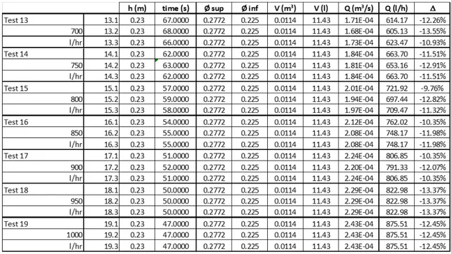
A rotameter is a device that measures the flow rate of a liquid in a closed tube. Before running the water hammer tests, the rotameter was tested and a calibration curve was obtained. For this purpose, the flow rate was measured in the flowmeter for different discharges and compared with the flow manually measured by the volumetric method. The volumetric method consists of measuring the time required for filling a container of known volume (11,43 litres).

Table 1 Summary of the rotameter calibration tests

h (m) time (s) Ø sup Ø inf V (m³) V (l) Q (m³/s) Q (l/h) ∆ Test 1 1.1 0.23 350.0000 0.2772 0.225 0.0114 11.43 3.27E-05 117.57 17.57% 100 1.2 0.23 365.0000 0.2772 0.225 0.0114 11.43 3.13E-05 112.74 12.74% l/hr 1.3 0.23 359.0000 0.2772 0.225 0.0114 11.43 3.18E-05 114.62 14.62% Test 2 2.1 0.23 268.0000 0.2772 0.225 0.0114 11.43 4.27E-05 153.54 2.36% 150 2.2 0.23 263.0000 0.2772 0.225 0.0114 11.43 4.35E-05 156.46 4.31% l/hr 2.3 0.23 265.0000 0.2772 0.225 0.0114 11.43 4.31E-05 155.28 3.52% Test 3 3.1 0.23 212.0000 0.2772 0.225 0.0114 11.43 5.39E-05 194.10 -2.95% 200 3.2 0.23 215.0000 0.2772 0.225 0.0114 11.43 5.32E-05 191.39 -4.30% l/hr 3.3 0.23 214.0000 0.2772 0.225 0.0114 11.43 5.34E-05 192.29 -3.86% Test 4 4.1 0.23 174.0000 0.2772 0.225 0.0114 11.43 6.57E-05 236.49 -5.40% 250 4.2 0.23 174.0000 0.2772 0.225 0.0114 11.43 6.57E-05 236.49 -5.40% l/hr 4.3 0.23 176.0000 0.2772 0.225 0.0114 11.43 6.49E-05 233.80 -6.48% Test 5 5.1 0.23 148.0000 0.2772 0.225 0.0114 11.43 7.72E-05 278.03 -7.32% 300 5.2 0.23 147.0000 0.2772 0.225 0.0114 11.43 7.78E-05 279.93 -6.69% l/hr 5.3 0.23 144.0000 0.2772 0.225 0.0114 11.43 7.94E-05 285.76 -4.75% Test 6 6.1 0.23 131.0000 0.2772 0.225 0.0114 11.43 8.73E-05 314.12 -10.25% 350 6.2 0.23 131.0000 0.2772 0.225 0.0114 11.43 8.73E-05 314.12 -10.25% l/hr 6.3 0.23 130.0000 0.2772 0.225 0.0114 11.43 8.79E-05 316.53 -9.56% Test 7 7.1 0.23 116.0000 0.2772 0.225 0.0114 11.43 9.85E-05 354.73 -11.32% 400 7.2 0.23 116.0000 0.2772 0.225 0.0114 11.43 9.85E-05 354.73 -11.32% l/hr 7.3 0.23 116.0000 0.2772 0.225 0.0114 11.43 9.85E-05 354.73 -11.32% Test 8 8.1 0.23 101.0000 0.2772 0.225 0.0114 11.43 1.13E-04 407.42 -9.46% 450 8.2 0.23 102.0000 0.2772 0.225 0.0114 11.43 1.12E-04 403.42 -10.35% l/hr 8.3 0.23 101.0000 0.2772 0.225 0.0114 11.43 1.13E-04 407.42 -9.46% Test 9 9.1 0.23 92.0000 0.2772 0.225 0.0114 11.43 1.24E-04 447.27 -10.55% 500 9.2 0.23 91.0000 0.2772 0.225 0.0114 11.43 1.26E-04 452.19 -9.56% l/hr 9.3 0.23 91.0000 0.2772 0.225 0.0114 11.43 1.26E-04 452.19 -9.56% Test 10 10.1 0.23 83.0000 0.2772 0.225 0.0114 11.43 1.38E-04 495.77 -9.86% 550 10.2 0.23 84.0000 0.2772 0.225 0.0114 11.43 1.36E-04 489.87 -10.93% l/hr 10.3 0.23 84.0000 0.2772 0.225 0.0114 11.43 1.36E-04 489.87 -10.93% Test 11 11.1 0.23 78.0000 0.2772 0.225 0.0114 11.43 1.47E-04 527.55 -12.07% 600 11.2 0.23 79.0000 0.2772 0.225 0.0114 11.43 1.45E-04 520.88 -13.19% l/hr 11.3 0.23 79.0000 0.2772 0.225 0.0114 11.43 1.45E-04 520.88 -13.19% Test 12 12.1 0.23 71.0000 0.2772 0.225 0.0114 11.43 1.61E-04 579.57 -10.84% 650 12.2 0.23 72.0000 0.2772 0.225 0.0114 11.43 1.59E-04 571.52 -12.07% l/hr 12.3 0.23 72.0000 0.2772 0.225 0.0114 11.43 1.59E-04 571.52 -12.07%

Rotameter measurements are plotted with volumetric measurements in Table 1 for a flow rate range from 100-1000 l/h. The correlation coefficient (R2) was calculated and the regression curve was obtained Figure 3.

Figure 4 Calibration curves obtained by the relationship between the flow rate measured in the rotameter

and the flow rate by volumetric measuring.

y = 0.8533x + 20.66 R² = 0.9993 0.0 100.0 200.0 300.0 400.0 500.0 600.0 700.0 800.0 900.0 1000.0 0 200 400 600 800 1000 1200 Fl ow ra te o bt ai ne d by v ol ume tri c me as uri ng (l /h )

Flow rate measured in the rotamenter (l/h)

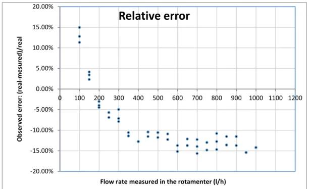
The relative error is positive for flow rates lower than 400 l/h and negative for higher flow rates. This error varies between 15% and -15%, tending to be constant for flow rates higher than 500 l/h Figure 4 and Figure 5.

Figure 5 Chart representing the relative error between the flow rate measured in the rotameter and the flow

rate by volumetric measurement.

TRANSIENT DATA COLLECTION

The instrumentation used for the measurement of the piezometric head time variation was composed of: two pressure transducers, an oscilloscope (Picoscope 3424) and a laptop computer. Seventeen tests have been carried out for different initial discharges and, for each discharge, the tests were repeated 20 times for obtaining the time-average. The water hammer was generated by instantaneous closure of the downstream end valve. Table 2 presents data obtained from the transient tests, namely the discharges and the corresponding maximum, minimum and amplitude of variation of the piezometric head, ΔHexp (which is the difference between the maximum piezometric head and the steady state one). Two values of celerity, the theoretical and the experimental, are also presented. The relative error between observed and theoretical Joukowsky overpressure, ΔHJ, are also presented.

-20.00% -15.00% -10.00% -5.00% 0.00% 5.00% 10.00% 15.00% 20.00% 0 100 200 300 400 500 600 700 800 900 1000 1100 1200 Ob se rv ed e rro r: ( re al -me su re d) /re al

Flow rate measured in the rotamenter (l/h)

Table 2 Table list of tests

Q Hsteady state

Hmax Hmin ΔHexp Celerity theor. Celerity exp. Joukowsky overpressure, ΔHJ Relative Error [L/h] [m] [m] [m] [m] [m/s] [m/s] [m] [%] 115 47.03 61.31 32.11 14.28 1270 1242.45 12.89 9.7% 155 46.95 65.70 27.28 18.74 1270 1255.26 17.55 6.3% 192.6 46.02 68.66 21.92 22.64 1270 1255.26 21.81 3.6% 235.6 46.74 74.67 17.58 27.93 1270 1255.26 26.68 4.5% 281.2 46.56 80.26 11.44 33.70 1270 1255.26 31.85 5.5% 314.9 46.44 84.90 6.72 38.46 1270 1255.26 35.67 7.3% 354.7 46.27 89.62 1.19 43.35 1270 1255.26 40.18 7.3% 406.1 46.01 94.61 -4.05 48.60 1270 1255.26 45.99 5.4% 450.6 45.94 99.24 -7.62 53.30 1270 1255.26 51.03 4.3% 491.8 45.57 102.60 -9.27 57.03 1270 1255.26 55.70 2.3% 523.1 45.70 135.44 -9.97 89.74 1270 1255.26 59.24 34.0% 574.2 46.17 152.52 -10.07 106.35 1270 1255.26 65.03 38.9% 614.3 46.29 174.60 -10.21 128.31 1270 1255.26 69.57 45.8% 614.3 46.47 174.68 -10.26 128.21 1270 1255.26 26.68 79.2% 709.6 47.00 172.51 -10.21 125.51 1270 1255.26 80.37 36.0% 752.8 47.48 167.84 -10.29 120.35 1270 1035.05 70.30 41.6% 801.7 47.65 160.17 -10.19 112.52 1270 1014.67 73.39 34.8%

The celerity was measured experimentally as: 𝒄𝒄𝒆𝒆𝒆𝒆𝒆𝒆=𝟒𝟒𝟒𝟒_𝑻𝑻

Equation 4

The celerity was measured experimentally as: ∆𝑯𝑯𝑱𝑱𝑱𝑱𝑱𝑱𝑱𝑱𝑱𝑱𝑱𝑱𝑱𝑱𝑱𝑱𝑱𝑱=𝒄𝒄𝒆𝒆𝒆𝒆𝒆𝒆_𝒈𝒈∆𝒗𝒗

Equation 5

where T= the wave period, L = the pipe length, g = the gravitational acceleration, ∆v = the mean velocity variation. In conclusion, the relative error was found using the following equation Eq. (3):

𝑹𝑹𝑹𝑹 =�𝑯𝑯𝒎𝒎𝒎𝒎𝒆𝒆− 𝑯𝑯_𝑯𝑯𝑱𝑱𝒔𝒔𝒆𝒆𝒎𝒎𝒔𝒔𝑱𝑱� − ∆𝑯𝑯𝑱𝑱𝑱𝑱𝑱𝑱𝑱𝑱𝑱𝑱𝑱𝑱𝑱𝑱𝑱𝑱𝑱𝑱

𝒎𝒎𝒎𝒎𝒆𝒆− 𝑯𝑯𝑱𝑱𝒔𝒔𝒆𝒆𝒎𝒎𝒔𝒔𝑱𝑱

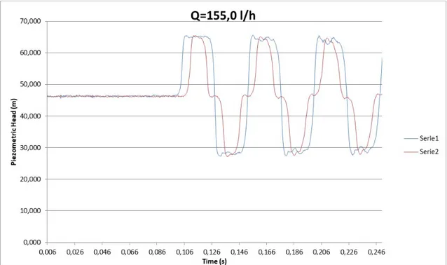
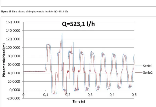
The following are graphs: Time history of the piezometric head from a range of 115 l/h up to a range of 801.7 l/h.

In particular, two cases are chosen to illustrate the phenomenon of the water hammer with and without cavitation: tests with discharges of 192.6 L/h and of 709.6 L/h (from Figure 6 to Figure 22). These tests were chosen to represent two different situations: a transient test without cavitation and a test with cavitation. In the first case, see Figure 6, it can be seen that at time t=0.2 s, the maximum values of the two pressure signals collected at two different locations (PT1 and PT2) are almost overlapped while in the second test, see Figure 16, two additional pressure peaks appear in the transient phase (Christopher E. 1998). As mentioned previously, this is due to the phenomenon of cavitation. For this setup, cavitation occurs for initial steady-state discharges higher than 523.1 L/h; after this value the R.E. increases. This confirms that the classic water hammer theory is not always valid in the presence of cavitation, given from Soares (2015) and Gale (2008).

Figure 7 Time history of the piezometric head for Q0=155.0 l/h

Figure 9 Time history of the piezometric head for Q0=235.6 l/h

Figure 11 Time history of the piezometric head for Q0=314.9 l/h

Figure 13 Time history of the piezometric head for Q0=406.1 l/h

Figure 15 Time history of the piezometric head for Q0=491.8 l/h

Figure 17 Time history of the piezometric head for Q0=574.2 l/h

Figure 19 Time history of the piezometric head for Q0=641.3 l/h

Figure 21 Time history of the piezometric head for Q0=752.8 l/h

Chapter 3

DISPLACEMENTS OF

THE PIPE SYSTEM

CAUSED BY A

TRANSIENT

PHENOMENON USING

THE DYNAMIC FORCES

MEASURED IN THE

LABORATORY

A severe form of water hammer is called surge, which is a slow-motion mass oscillation of water caused by internal pressure fluctuations in a system, described by Shamloo H (2015). This can be pictured as a slower “wave” of pressure arising within the system. If not controlled, it can yield the following results: damage to pipes, fittings, and valves, which in turn causes leaks and life shortening of the system Given by Malesinszka A. (2015).

This work was published in the journal Measurement and Control (United Kingdom) (2018).

INTRODUCTION

This thesis shows the use of equations describing the movement of suspended mass focused on the beam to calculate the displacement of the pipelines under the action of dynamic forces. This approach will allow the calculation, as far as possible, of the actual displacement of the pipeline in the direction of flow change. This is very important information for designers calculating and selecting parameters of fixed points Ghidaoui M. (2005).

One of the factors that affect the reliability of an installation is its proper fastening to the structure of the building or other supporting components. This is especially important for installations which are exposed to dynamic loads. An example of an installation with the necessary high reliability exposure to dynamic loads is a fire protection system. The selection of fastening elements for such an installation depends on the force that the fastener can carry. Unfortunately, it is usually assumed that the force is applied statically. Therefore, it is important to implement numerical models for the calculation of the displacements for the dynamic system, and to compare them with physical models.

The measurements made, (in order to calculate the parameters of the pipe-water system), are necessary to calculate displacements based on the equation using the natural frequency for the entire system (i.e. the walls of the pipe and water filling the pipe). Such approach allows the impact on displacement to take in account not only the coefficient of elasticity of the pipe walls, but also the bulk modulus of the water filling the pipe. Considering the mutual influence of both coefficients of elasticity (by calculating the natural frequency of oscillations) will allow a more accurate description of the phenomenon. The described problem does not finish solving the whole task. Currently, further research is planned to confirm the validity of the assumptions made, as well as to conduct measurements for pipes of various materials, with different wall thicknesses and the proportions of wall thickness and inside diameter, as well as for liquids with different densities, descibed by Edwards JE (2015). Such an examination will allow for the development of a computational scheme, which in a simple way will allow, for example, engineers to calculate real ranges of displacements of pipe systems caused by transient phenomena. This knowledge, in turn, will allow adequate protection of pipe systems against damage, thanks to the appropriate pipe support selection.

EXPERIMENTAL FACILITY IN LABORATORY

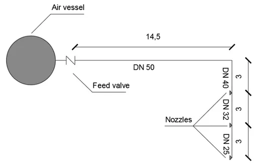
This thesis presents and improves in detail the study which was presented in a simple form by Malesinszka (2015). The draft of the test stand concerned the simple scheme of a fire protection system, consisting only of the distribution pipe and one straight pipe (made up of three different diameters), armed with three nozzles. A simple geometric scheme allowed for an initial analysis and identification of phenomena accompanying the hydraulic shock wave propagation. The pipe system was designed in accordance with applicable standards. A scheme of the designed installation is presented in Figure 23 and Table 3.

Figure 23 Scheme of the laboratory test stand.

A system of steel of various outer diameters D0 and wall thickness e

Table 3 Properties of steel pipes used in the experiment.

No

Nominal

diameter

DN [mm]

Outer

diameter

D

[mm]

Wall

thickness

e [mm]

Individual

celerity c

[m/s]

Pipe

length

L [m]

1

50

60.3

3.65

1280

14.5

2

40

48.3

3.25

1280

3.0

3

32

42.3

3.25

1280

3.0

4

25

33.7

3.25

1280

3.0

The installation system that was accepted for the study was not filled with water. It was a model of an air system device used to protect the space of construction objects from the risk of frost or water evaporation. The installation system was equipped with three upright nozzles. The nozzles were placed one on each section of constant diameter DN40,

DN32 and DN25. The test stand for the water hammer analysis was

constructed to perform the experiments, using the measuring system and recording of fast-changing pressure values.

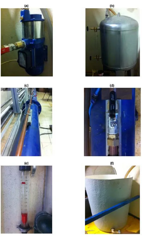
The model was supplied with water via a pressure increasing station Figure 24 and Figure 25. The water in the tank was refilled from a water supply system. Permanent steady flow conditions established in the model of the system were made possible by the use of a water-air tank which had a capacity of 300 dm3_{. The model was connected to the}

compressor, allowing an increase in the initial pressure in the system to the value of 5.5 bar, see Figure 25.

Figure 24 Upright

nozzle installed in the pipe

Figure 25 Pressure increasing station with the compressor.

The measurement and analysis of the results was for a simple water hammer only, i.e. with pressure wave transition time T always higher than the valve opening time tz. The experiment was performed at an

average temperature of 281 K (Puntorieri. P. 2017).

The values of the forces impacting the components of the system were evaluated as follows:

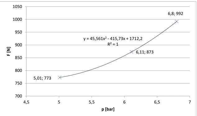
1. In the first step, the forces were measured by a means of dynamometers (for a detailed description of the measurements and the results obtained, see Malesinszka A. (2015). Figure 26 shows only the relationship between the measured forces and the pressure in the cross-section in which the forces were measured.

Figure 26 Relationship between the measured forces and the pressure in the cross-section in which the

forces were measured

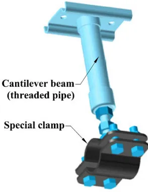
2. Then, in the same section after removing the dynamometers, a fixed support was installed, constructed from a special clamp hung on an 80 cm threaded, see Figure 27. On this threaded pipe, after special preparation, a strain gauge was attached, which then allowed the stress measurements to take place, see Figure 28. This fixed support is working as a cantilever beam with a point mass suspended at its end. The threaded pipe is considered as a cantilever beam, and the steel pipe with water as a suspended mass. 5,01; 773 6,8; 992 6,11; 873 y = 45,561x2_{- 415,73x + 1712,2} R² = 1 700 750 800 850 900 950 1000 1050 4,5 5 5,5 6 6,5 7 F [ N] p [bar]

Figure 27 Scheme of a fixed support on which the model was suspended.

In addition, measurement involved the concurrent measuring of a pressures and flow rate, and also the opening time of the feed valve. This measurement guaranteed a comparison of the water hammer phenomenon for the same (or very similar) boundary conditions. The valve opening time was closely linked to the valve opening angle. The measurement of voltage obtained from the potentiometer, mechanically coupled with the valve hand wheel, was used to register the changes during the opening angle of the feed valve. This procedure ensured a voltage proportional to the angle of rotation of the valve hand wheel. The turbine flow meter type TUV-1210, which could record the counted flow units, was used for flow measurement.

All the recorded values were recorded using a computer that was equipped with software that controlled the measurement process and all further processing. The basic software was developed in the “C” language, using “Turbo C” program for compilation and subroutine statements. Two versions of the software were designed: a version used to record the measurements, and a version used to analyze the measurement results and the recorded value outputs.

CASE STUDY

The analysis included three work variants of the examined installation in the laboratory. Variant 1 – one nozzle opened, variant 2 – two nozzles opened, and variant 3 – three nozzles opened.

Strain gauges installed on the cantilever beam of the fixed support allowed the calculation of the mass that was suspended on the beam, and then using the equation of oscillatory motion, the beam displacement was calculated for the suspended installation.

Before any measurements were taken, the strain gauges attached to the cantilever beam of the fixed support was calibrated, and the basic strength characteristic of the applied cantilever, which was necessary for calculation of the mass suspended on the beam, was determined. Two wire strain gauges with the following parameters were attached to the beam:

– nominal resistance Rnom = 600 Ω,

– transformation constant K = 2.62, – active length l = 10 mm

Both strain gauges were combined in a “bridge” system. The half-bridge system was used due to the measured parameter. In this system, one strain gauge was under compression and the other under tension. The strain gauges were attached to the previously prepared surface (the surface was leveled and cleaned). The place of attaching the strain gauges is shown in Figure 28. The strain gauges were attached as close as possible to the place where the beam was fastened, so as to minimize

the effect of changing the length of the bent beam on the accuracy of strain gauge measurements. On the diagonal of the bridge to obtain the change in voltage ΔU, which depended on the resistance change ΔR/R:

∆𝑈𝑈 𝑈𝑈 = 1 2 ∆𝑅𝑅 𝑅𝑅 Equation 7 where:

U = voltage of bridge powering [V],

∆𝑅𝑅 = 𝑅𝑅𝑛𝑛𝑛𝑛𝑛𝑛𝐾𝐾𝐾𝐾

Equation 8

Ε = relative elongation of strain gauges in the range of elastic strains, ε

= 0.001, thus: ∆𝑈𝑈 𝑈𝑈 = 1 2 ∗ 2.62 ∗ 0.001 = 0.0013 Equation 9

With the bridge powered by a voltage U of 5V, a strain gauges bridge input signal imbalance is obtained, and is equal to:

∆𝑈𝑈 = 5 ∗ 0.0013 = 0.0065 V = 6.5 mV

Equation 10

By strengthening the direct current, having for example an amplification of L = 1000, it is possible to obtain an input signal of 6.5 V with 1 kN of force applied to the end of the cantilever beam in question.

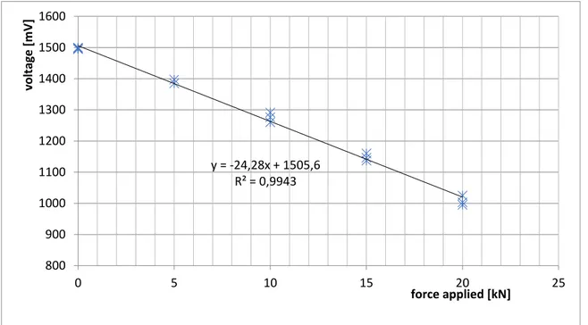
Strain gauges calibrating was carried out by applying a force of known value [kN], and then reading the values of voltage [mV] corresponding to these known force values and their corresponding voltage changes. Since the relationship presented is linear, a best fit of the variability function was determined by the least squares method Figure 29.

Figure 29 Strain gauges calibrating, readout of voltage value for known applied force value.

To calculate the strength parameters of the cantilever threaded pipe beam of the fixed support, it is necessary to know the basic geometrical and material parameters of the beam:

– inner diameter d = 33 mm,

– outer diameter D = 39 mm (below the thread), – beam length L = 80 cm,

– elastic modulus for steel E = 2.09*105 _MPa.

Beam strength parameters were then calculated based on the above data values:

– moment of inertia for beam cross-section: 𝐽𝐽 =₃₂𝜋𝜋 (𝑔𝑔4_{− 𝑑𝑑}4_{) = 11.069 𝜌𝜌𝑚𝑚}4 Equation 11 – cross-section modulus: 𝑊𝑊 =_{16 �}𝜋𝜋 𝑔𝑔4_𝑔𝑔− 𝑑𝑑4� = 5.677 𝜌𝜌𝑚𝑚3 Equation 12 y = -24,28x + 1505,6 R² = 0,9943 800 900 1000 1100 1200 1300 1400 1500 1600 0 5 10 15 20 25 vo lta ge [m V] force applied [kN]

– beam cross-section:

𝐴𝐴 =𝜋𝜋₄(𝑔𝑔2_{− 𝑑𝑑}2_{) = 3.39 𝜌𝜌𝑚𝑚}2

Equation 13

– with a beam length of L = 80 cm, 271 cm3 _{of beam material}

net volume is obtained.

CALCULATION OF THE DEFLECTION OF THE CANTILEVER BEAM – STATIC FORCE APPLIED AT THE END OF THE CANTILEVER

The displacement of the end of the beam as a result of the static action of the concentrated force, F, according to the material mechanics theory can be calculated from the relationship:

𝑓𝑓 = 𝐹𝐹𝐿𝐿_{3𝐸𝐸𝐽𝐽}3

Equation 14

where:

f = displacement of the end of the cantilever beam (deflection) [m], F =

concentrated force [N], L = beam length [m], E = modulus of elasticity of the beam [Pa], J = modulus of inertia of the beam [m4_].

For the scheme presented in Figure 28, in the first stage of the test, the components of the force caused by the water hammer pressure wave were measured using dynamometers, given by Malesinszka A. (2015). The measured force components were used at this point to calculate the displacement of the beam end after the static force was applied at the end of the beam, i.e. the threaded pipe of the fixed support.

The cantilever beam was 80 cm long. For that particular beam length and the calculated strength parameters in Table 4, the deflection of the cantilever beam based on the calculated resultant forces was determined.

Table 4 Calculated deflections for the acting resultant forces

Variant

Force F [N]

Deflection f [cm]

I

773

0.57

II

992

0.73

III

873

0.64

USE OF THE EQUATION OF THE OSCILLATORY MOTION FOR MAXIMUM DEFLECTION

DETERMINATION OF THE CANTILEVER BEAM

In the first step, the frequency of the natural oscillations of the pipe system not filled with water was measured in the laboratory. Oscillation inductions were forced by hitting with a soft pad. The oscillations constitute periodical motion in which all the points of the oscillating system, after a fixed time interval, would return to the initial value in a reproducible manner. This time interval is called the period of oscillation, and it is denoted by the letter T. The reciprocal of the period

1/T= f is called the frequency of oscillations. The frequency of natural

oscillations of beam + mass f [Hz] system was measured, which gives: – angle velocity

𝜔𝜔 = 2𝜋𝜋𝑓𝑓 [𝑟𝑟𝑟𝑟𝑑𝑑/𝑠𝑠]

Equation 15

– angle velocity of beam with susceptibility k, and mass concentrated at the end of the beam

𝜔𝜔 = �_𝑚𝑚𝑘𝑘

Equation 16

thus

𝑚𝑚 =_𝜔𝜔𝑘𝑘₂

in order to obtain the characteristic of oscillations, two records of suppressed oscillations, “dr1” and “dr2”, were made.

Figure 30 Course of forced oscillation for an empty pipe, “dr1”

To register “dr1” Figure 30, 9 cycles took 1430 - 350 = 1080 recorded points (x, y = counted non scaled impulses). Each registered point lasts 2 ms, thus 9 cycles lasted 2.16 seconds which corresponds to:

– oscillations period T = 2.16/9 = 0.24 [s], – oscillations frequency f = 4.17 [Hz], – angle velocity ω0 = 26.17 [rad/s].

On the basis of the course of the forced oscillation for the empty pipe,

"dr2", similarly to the first case "dr1", 10 cycles were taken from the

recorded characteristic, which took 1430 - 255 = 1175 registered points (x, y = counted non scaled impulses) 2.35 seconds, corresponding to:

– oscillation period T = 2.35/10 = 0.235 [s], – oscillation frequency f = 4.25 [Hz], – angle velocity ω0 = 26.72 [rad/s].

Mean value of angle velocity for the dry system is ω0avg = 26.45 [rad/s].

Finally, it is possible to calculate the mass suspended on the cantilever beam assuming that the suspension is at its end point. Hence, the constant of beam susceptibility was calculated from k = 3EJ/L3 _[N/m],

where L = beam length. According to the Equation 10we know that 𝑚𝑚 = 𝑘𝑘/𝜔𝜔^2 , where k = 135 [kN/m] and ω = 26.45 [rad/s] are the values calculated for the examined system. Thus, we obtain mass value m = 193 [kg].

In the same manner, using the measured characteristics, the following was established for the wet pipes:

– oscillation period T = 0.28 [s]; – oscillation frequency f = 3.57 [Hz];

– angle velocity ω = 22.4 [rad/s], calculated from Equation 8; – mass m = 269 [kg], calculated from Equation 10.

As the value of the concentrated mass suspended at the end of the cantilever beam is known, it was possible to analyze the oscillations forced by a sudden application of force – a response of the system to the pressure wave propagation. Forcing the oscillating system motion is a certain process, and as known, its nature can be of an aperiodic process character, in particular the transition one.

Then the mathematical model of the system with suppressing takes the following form:

𝑚𝑚𝜕𝜕̈ + 𝜌𝜌𝜕𝜕̇ + 𝑘𝑘𝜕𝜕 = 𝐹𝐹(𝜕𝜕)

Equation 18

where force F(t) may be aperiodic, and also a discontinuous function. To determine the motion of the oscillating system affected by the action of aperiodic extortions, the response of the system on two elementary forces can be analyzed, i.e. the unit impulse and the unit step. The impulse is a measure of the impact of short-term forces, e.g. the closing and quick opening of the feeding valve. The step is a response to the force of the constant value suddenly applied to the physical system, e.g. a heat shock caused by a sudden temperature change.

In the case of the water hammer phenomenon, we are dealing with an applied instantaneous force. A measure of the impact of short-term forces is impulse S, i.e.

𝑆𝑆 = � 𝐹𝐹(𝜕𝜕)𝑑𝑑𝜕𝜕𝑡𝑡2 𝑡𝑡1

When the time Δt of force F(t) operation is very short, as it is in the case of pressure wave propagation, it is an instantaneous force. The solution of the equation of suppressed oscillatory motion induced by instantaneous force, taking into account the subcritical suppression, is the following function:

𝜕𝜕(𝜕𝜕) =_{𝑚𝑚𝜔𝜔}𝑠𝑠 𝐷𝐷𝑒𝑒 −𝑏𝑏𝑡𝑡_{𝑠𝑠𝑠𝑠𝑠𝑠𝜔𝜔} 𝐷𝐷𝜕𝜕 Equation 20 where:

x = displacement of the end of the cantilever beam in time S = impulse caused by instantaneous force action, S = F0Δt, m = mass, in this case calculated based on measured characteristics

of mass value for a wet installation, m = 269 [kg],

ωD =frequency of suppressed free oscillations (natural frequency),

𝜔𝜔𝐷𝐷= �𝜔𝜔02− 𝑏𝑏2

Equation 21

ω0 = natural oscillations frequency,

b = normalized suppression coefficient, b = c/2m,

c = viscous suppression coefficient, related to the suppressive properties

of viscoelastic material,

𝜌𝜌 =𝑔𝑔𝑘𝑘_𝜔𝜔

Equation 22

𝜔𝜔 = 𝜔𝜔0

Equation 23

g = number characterizing the suppression properties of the beam,

𝑔𝑔 = 𝐼𝐼𝑚𝑚𝐸𝐸∗_{/𝑅𝑅𝑒𝑒𝐸𝐸}∗

Equation 24

ImE = imaginary part of complex elastic modulus, ReE = real part of complex elastic modulus,

E = complex elastic modulus, i.e. variable over time, k = number characterizing elastic properties of the beam,

𝑘𝑘 = 𝐴𝐴𝑅𝑅𝑒𝑒𝐸𝐸∗_/𝑙𝑙

On the basis of the experiments conducted, and by calculating certain values characteristic of the analyzed system, it is possible to derive an equation of suppressed oscillatory motion caused by the activity of the instantaneous force – pressure wave propagation.

In order to derive an equation of suppressed oscillatory motion, the relationship for TD may be used, which is defined as the time interval

between two successive peaks in the same direction. The TD value is

constant in time and can be calculated from the following relationship:

𝑇𝑇𝐷𝐷= 2𝜋𝜋 �𝜔𝜔02− 𝑏𝑏2

Equation 26

Explanations are similar to those in Equation 14

Having the measured characteristics for the experiment, it is now possible to determine the value of TD = 0.29 s. After converting the

above relationship, it is possible to calculate the standardized suppression coefficient b = 5.69 [rad/s], and ωD = 21.66 rad/s.

For the assumed unit impulse inducing system oscillation, the equation of the change of displacement versus time takes the form (h and x are the same parameters describing displacement of the end of the cantilever beam): ℎ(𝜕𝜕) = _{𝑛𝑛𝜔𝜔}1 𝐷𝐷𝑒𝑒 −𝑏𝑏𝑡𝑡_{𝑠𝑠𝑠𝑠𝑠𝑠𝜔𝜔} 𝐷𝐷𝜕𝜕 Equation 27 m = 269 kg, b=5.69 rad/s, ωD = 21.66 rad/s, TD = 0.29 s ℎ(𝜕𝜕) = 1.716 ∗ 10−4_𝑒𝑒−5.69𝑡𝑡_{𝑠𝑠𝑠𝑠𝑠𝑠21.66𝜕𝜕} Equation 28

In the case of a water hammer, it was assumed that the concentrated force F was acting in infinite time. So, it is assumed that the impulse S is equal to the force F.

According to the equation of the oscillatory motion, the maximum displacement xmax is as follows:

𝜕𝜕𝑛𝑛𝑚𝑚𝑚𝑚=_{𝑚𝑚𝜔𝜔}𝑆𝑆 𝐷𝐷𝑒𝑒 −𝑏𝑏𝑏𝑏 2𝜔𝜔𝐷𝐷 𝑓𝑓𝑓𝑓𝑟𝑟 𝜕𝜕 = 𝜋𝜋 2𝜔𝜔𝐷𝐷= 0.07 𝑠𝑠 Equation 29

Assuming S = F, xmax was calculated for the force values listed in Table

5.

Table 5 Calculated deflections for the acting resultant forces

F1 (N) X1 (cm) F2 (N) X2 (cm) F3 (N) X3 (cm)

773 8.78 992 11.26 873 9.91

Knowing the function describing end of the cantilever beam displacement, the pipe of the installation displacement is known as well.

MATLAB PACKAGE IMPLEMENTATION

To calculate the change in displacement of the end of the supporting beam for unit impulse versus time, the MATLAB package was used. For this purpose, the following oscillation function was created: function [x, t] = oscillation (S, m, omega0, Td, figure), which requires the following input parameters:

S = value of unit impulse [N],

m = mass concentrated at the end of beam [kg], omega0 = angular velocity [rad/s],

Td = contractual period [s],

figure = parameter specifying whether or not to create a figure.

The function returns two output values:

x = the value of maximum displacement [cm],

t = time, after which the value of maximum displacement occurred.

To solve the problem, all of the values needed for equation 26 must be calculated. Based on the ɷ0 and Td parameters, the value of the

normalized suppression coefficient (b) is determined. Then, by using this value, the value of ɷD is calculated. After calculating all the

necessary values, the symbolic variable t is created, and equation 26 is built using the provided and calculated values.

The built equation is solved to find the global minimum using the GlobalSearch class and the corresponding settings for the optimization problem of one variable, from Barton N. (2013).

Finally, the graph of the function is plotted, and the maximum value found (the minimum value determined by the above optimization problem) is marked on the graph, and the two output parameters are returned from the function.

The function block diagram is shown in Figure 31. Example of a function call:

For the following input parameters: S = 992 N, m = 269 kg, ω0 = 22.4

rad/s, Td = 0.29 s output parameters were obtained: x = 11.661 cm, t =

0.060653 s and the graph of the function was as Figure 32.

Chapter 4

EQUIVALENT

CELERITY IN WATER

HAMMER FOR

SERIALLY CONNECTED

PIPELINES

This thesis presents the results of research on a physical model that confirms the dissimilarity of celerity values for pipes of different diameters and considers the relationship of diameter size changes with the length of the combined sections. In the case of piping systems, instead of computing the celerity c, the equivalent celerity ce must be

determined. For this purpose, an equation for natural vibration analysis has been proposed as a simple and fast method for computing the equivalent celerity of piping systems.

The analytically computed values were compared with values obtained from actually measured characteristics.

In this way, the satisfactory compliance of the compared values, and thus the validity of applying derived equations for a simple estimation of the equivalent celerity in piping systems, can be confirmed. This allows the computation of the maximum pressure increase in the system.

Using natural vibration analysis to calculate the equivalent celerity, it is possible to estimate the basic parameters of water hammer in a fast and easy way, and among other things, the expected maximum pressure increase without having to use complex computer programs to simulate water hammer.

This in turn can translate into a fast verification of the assumed parameters and pipe configuration in the rebuilt or modernized network for estimating the water hammer phenomenon as a function of connected pipes of different diameters, different lengths and different material compositions.

To facilitate the use of the equations, an algorithm implemented in MATLAB has been presented that allows the specification of the value of the celerity ce for any number of connected pipes.

This work was presented at the WIT Transactions on Engineering Sciences conference in Prague (2018) and is being published in the ASCE journal.

LINEAR ANALYSIS METHODS

To simulate the water hammer phenomenon, linear analysis methods can be used, provided that the pulsing in the relevant system is a periodic motion. This is confirmed by harmonic analysis of the phenomenon, using the classical oscillation equations, and limiting it to the case of damped natural vibrations. Vibrations are periodic movements in which all points of the vibrating system repeatedly return to the initial state after a fixed time interval. The simplest vibrating motion is the harmonic motion. Any periodic vibration can be formed by the superposition of the basic harmonic vibrations of the same period and, in a limited case, from an infinite number of higher harmonic vibrations of appropriately selected amplitudes and phases. Vibrations triggered by the action of a single pulse are natural vibrations. An example of this type of vibration is the water hammer formed under the influence of a single pulse, such as, for example, the sudden closure of a valve.

In an attempt to predict certain parameters of the water hammer phenomenon, one can use a theory based on the natural vibrations of the system utilizing the equations of fluid mechanics.

Often, when using equations governing the variable flow of liquid in the pipeline system, the solution reduces to a function of time. Thus, the analysis is limited only to a temporary state or the method of triggering this state. According to harmonic analysis of the water hammer phenomenon, a variable flow may sometimes be referred to as periodically pulsing or showing its own vibration. With such a description of the phenomenon, the solution of the equations allows the frequency to be determined (i.e. one can search for solutions directly specifying a steady pulsation cycle). In this case, achieving a uniform rate of the pulsation cycle is important.

Frequency-dependent factors, such as friction or wave celerity, have a major impact on the dynamic behaviour of liquids in pulsating conditions as a result of extraordinary energy dissipation or due to fluctuations of wave celerity.

Borrowing methods from the theory of linear vibrations requires reducing the equations describing the course of the phenomenon to a linear form Pipes (1958). To this end, the differential equation of motion and continuity is adopted in simplified form, i.e. it is assumed that the average flow parameters are "constant". Thus, their derivatives are both zero, and the friction is reduced to a linear form. This way, a particular solution of equations is obtained - a solution resulting in algebraic equations related to the pipeline parameters and boundary conditions.

Simplified equations of motion and continuity take the following form, Wylie (1993): 𝜕𝜕𝐻𝐻 𝜕𝜕𝜕𝜕 + 1 𝑔𝑔𝑔𝑔 𝜕𝜕𝑔𝑔 𝜕𝜕𝜕𝜕 + 𝜆𝜆𝑔𝑔𝑛𝑛 2𝑔𝑔𝑔𝑔𝐴𝐴𝑛𝑛= 0 Equation 30 𝜕𝜕𝑔𝑔 𝜕𝜕𝜕𝜕 + 𝑔𝑔𝐴𝐴 𝜌𝜌2 𝜕𝜕𝐻𝐻 𝜕𝜕𝜕𝜕 = 0 Equation 31

The use of these equations in the linear vibration analysis after the introduction of the hyperbolic functions allows the derivation of equations describing the amount of pressure and flow as a function of position in the pipeline:

𝐻𝐻(𝜕𝜕) = 𝐻𝐻𝑈𝑈𝜌𝜌𝑓𝑓𝑠𝑠ℎ𝛾𝛾𝜕𝜕 − 𝑍𝑍𝐶𝐶𝑔𝑔𝑈𝑈𝑠𝑠𝑠𝑠𝑠𝑠ℎ𝛾𝛾𝜕𝜕

Equation 32

𝑔𝑔(𝜕𝜕) = −𝐻𝐻_𝑍𝑍𝑈𝑈

𝐶𝐶𝑠𝑠𝑠𝑠𝑠𝑠ℎ𝛾𝛾𝜕𝜕 + 𝑔𝑔𝑈𝑈𝜌𝜌𝑓𝑓𝑠𝑠ℎ𝛾𝛾𝜕𝜕

Equation 33

Equation 29 and Equation 30 are equations of pressure and flow transfer. Using the above equations allows the computation (after appropriate substitutions and transformations) of the equivalent celerity thanks to the linking of pipe properties (Ai, ci, Li) with the natural

frequency of the system. As will be shown, the use of the method of natural vibration provides a simple solution to this problem. Further discussion will focus on the serial connection of two and three pipes made of different materials and for different ratios of diameters and lengths of connected sections.

For the correct solution of the issue, a correct definition of the boundary conditions of system operation is important.

Figure 33 shows an example of a serial connection of two pipes. According to the presented scheme, the boundary conditions are as follows:

HD1 = HU2 and QD1 = QU2

Figure 33 Scheme of a serial connection of two pipes.

For any point of the pipe, an equation for the transfer of pressure and flow can be written as given in Equation 29 and Equation 30.

Using the boundary conditions and the fact that the pipes are serially connected, the following equation can be obtained:

−𝑍𝑍_𝑍𝑍𝑐𝑐1

𝑐𝑐2𝜕𝜕𝑟𝑟𝑠𝑠ℎ𝛾𝛾1𝐿𝐿1𝜕𝜕𝑟𝑟𝑠𝑠ℎ𝛾𝛾2𝐿𝐿2= 1

Equation 35

To obtain only the dependencies between geometric parameters of the connected pipes and the vibration frequency of the entire system from the equation above, adequate substitutions for ZC and γ must be made.

For this purpose, it should be noted that if the vibration pulsation has a regular amplitude at each point x of the hydraulic system, the size of the real part of s must be zero. The propagation constant thus takes the following form:

𝛾𝛾 = �𝐶𝐶𝜔𝜔(−𝜔𝜔𝐿𝐿𝑏𝑏+ 𝑠𝑠𝑅𝑅)

Equation 36

The proper impedance is:

𝑍𝑍𝐶𝐶= −_{𝐶𝐶𝜔𝜔}𝑠𝑠𝛾𝛾

For a system without friction:

𝛾𝛾 = �−𝐶𝐶𝜔𝜔2_{𝐿𝐿𝑏𝑏 = 𝜔𝜔𝑠𝑠�𝐶𝐶𝐿𝐿𝑏𝑏}

Equation 38

Substituting C and Lb with dependencies, C = gA/c2and Lb = ζ/(gA)

(Brown 1969 ), ( (Zielke 1972), the following is obtained:

𝛾𝛾 =𝜔𝜔𝑠𝑠_𝜌𝜌

Equation 39

𝑍𝑍𝑐𝑐=_{𝑔𝑔𝐴𝐴}𝜌𝜌

Equation 40

Substituting the dependencies Equation 36 and Equation 37 into Equation 32, it follows: 𝜕𝜕𝑟𝑟𝑠𝑠ℎ𝜔𝜔𝐿𝐿_𝜌𝜌 1 1 𝑠𝑠 ∙ 𝜕𝜕𝑟𝑟𝑠𝑠ℎ 𝜔𝜔𝐿𝐿2 𝜌𝜌2 𝑠𝑠 = − 𝜌𝜌2𝐴𝐴1 𝜌𝜌1𝐴𝐴2 Equation 41

Using the generalized Euler’s formula:

tanh 𝑧𝑧𝑠𝑠 = _{cosh 𝑧𝑧𝑠𝑠}sinh 𝑧𝑧𝑠𝑠

Equation 42

where:

sinh 𝑧𝑧𝑠𝑠 = 𝑠𝑠 sin 𝑧𝑧 , cosh 𝑧𝑧𝑠𝑠 = cos 𝑧𝑧

Equation 43

The relation Equation 38 can be written as follows:

𝑠𝑠 �𝜕𝜕𝑟𝑟𝑠𝑠 𝜔𝜔𝐿𝐿_𝜌𝜌1 1 � 𝑠𝑠 �𝜕𝜕𝑟𝑟𝑠𝑠 𝜔𝜔𝐿𝐿2 𝜌𝜌2 � = − 𝜌𝜌2𝐴𝐴1 𝜌𝜌1𝐴𝐴2 Equation 44 𝜕𝜕𝑟𝑟𝑠𝑠 𝜔𝜔𝐿𝐿_𝜌𝜌 1 1 𝜕𝜕𝑟𝑟𝑠𝑠 𝜔𝜔𝐿𝐿2 𝜌𝜌2 = 𝜌𝜌2𝐴𝐴1 𝜌𝜌1𝐴𝐴2 Equation 45

Solving the equation above with regard to ω, the equivalent celerity of the pressure wave ce for the entire pipeline can be determined. Because

2𝑇𝑇 = 4𝐿𝐿_𝜌𝜌 𝑒𝑒 = 2𝜋𝜋 𝜔𝜔 Equation 46 hence: 𝜌𝜌𝑒𝑒=2_{𝜋𝜋 𝐿𝐿𝜔𝜔} Equation 47

where L = L1 + L2, is the length of the entire pipeline.

It should be noted that using the dependency Equation 42 substantially simplifies and speeds up the computation of the equivalent celerity of pressure oscillation changes upon reaching the natural vibrations of the system. Equation 42 is only true for a system consisting of two pipes. The analysis of natural vibration oscillations for three pipes connected in series requires the introduction of a new dependency in accordance with the scheme described above. Using Equation 29 and Equation 30 for computation purposes requires the knowledge of pressure distribution in sequential cross-sections of the analysed pipe system, which would be quite problematic to obtain.

For the system consisting of 3 pipes, as shown in Figure 34, one must correctly determine the boundary conditions and then, proceeding similarly as for the system consisting of 2 pipes, derive a new dependency.

Finally, for the system consisting of three pipes, the following equation is obtained: 𝜌𝜌1𝐴𝐴2 𝜌𝜌2𝐴𝐴1tan 𝜔𝜔𝐿𝐿1 𝜌𝜌1 tan 𝜔𝜔𝐿𝐿2 𝜌𝜌2 + 𝜌𝜌1𝐴𝐴3 𝜌𝜌3𝐴𝐴1tan 𝜔𝜔𝐿𝐿1 𝜌𝜌1 tan 𝜔𝜔𝐿𝐿3 𝜌𝜌3 + 𝜌𝜌2𝐴𝐴3 𝜌𝜌3𝐴𝐴2tan 𝜔𝜔𝐿𝐿2 𝜌𝜌2 tan 𝜔𝜔𝐿𝐿3 𝜌𝜌3 = 1 Equation 48

Similarly, as was the case with two pipes, the solution of the equation with respect to ω allows for the computation of the equivalent celerity ce.

MATERIALS AND METHODS

To validate the use of the natural vibration method to determine the equivalent celerity in water hammer research, a series of tests on the measuring station as shown in Figure 35 has been conducted.

Figure 35 Measuring station for the research of water hammer 1 – reducing valve; 2 – hydrophore tank;

3, 4, 5 – tested pipes with variable geometric parameters (diameter, length of tested section); 6 – measuring vessel; 7, 8, 9, 10 – pressure sensors; 11 – shut-off valve with closing time meter, 12 – amplifier; 13 – PC with analog card; 14 – regulated pipe clamped to the ground.

For testing purposes, pipes of geometric parameters as listed in Table 6 have been used.

Table 6 Properties of pipes used for testing.

No. Symbol of pipe used for testing

D0 e C

[mm] [mm] [m/s]

Polyethylene MDPE pipes

1 P1 50 (1.97 in.) 4.6 (0.18 in.) 390 (1,279.5 fps) 2 P2 40 (1.57 in.) 3.7 (0.14 in.) 390 (1,279.5 fps) 3 P3 32 (1.26 in.) 3.0 (0.12 in.) 390 (1,279.5 fps) 4 P4 25 (0.98 in.) 2.3 (0.09 in.) 390 (1,279.5 fps) Steel pipes 5 S1 48 (1.89 in.) 3.0 (0.12 in.) 1,280 (4,199.5 fps) 6 S2 42 (1.65 in.) 3.5 (0.14 in.) 1,280 (4,199.5 fps) 7 S3 33.5 (1.32 in.) 3.5 (0.14 in.) 1,280 (4,199.5 fps) 8 S4 27 (1.06 in.) 3.0 (0.12 in.) 1,280 (4,199.5 fps)

The closing time of the ball valve with adjustable spindle angle was determined by an electronic meter with an accuracy of 10-3 _s.

Depending on the type of measured pipe, the closing time of the ball valve varied: for steel pipes, tz = 0.016 - 0.023 s; for polyethylene pipes, tz = 0.025 - 0.035 s (depending on the initial opening degree of the ball

valve).

Measurements and analysis of the results apply only to a simple water hammer, i.e. one in which the time of the pressure wave T is always greater than the bar closing time tz <T. In addition, the bar closing time

tz is always shorter than the returning time tr of the first reflected

pressure wave to the outlet side tz < tr.

The experiment was performed at a constant temperature of 8°C± 2% (46.4°F). Maintaining a fixed temperature was especially important for polyethylene pipes due to the effects of temperature on their mechanical properties, given by Janson (1995).

The characteristics of the water hammer pressure p(t) were defined in the three measuring points of the pipeline. The pressure sensors have been tarred so that the voltage value for the known pressure p0 is zero. The measuring range of the sensors (12 - 20 bar ± 0.1 bar (174.04 - 290.06 psi)) has been selected according to the stream velocity v0 of

uniform flow and the expected maximum pressure at the measuring points.

The water stream pressure before the water hammer was measured at the outlet of the pipeline. The pressure was 4.5 - 5.0 bar± 0.1 bar (65.26 - 72.51 psi). The average velocity v0 of fixed flow (determined in the

calculation section of the pipeline and the section at the end of the pipeline) and the pressure p0 were chosen so as to prevent the

occurrence of cavitation during water hammer.

The study was conducted for five variants of connected pipes, see Figure 36.

RESULTS AND DISCUSSION

In the conducted measurements, a number of pressure characteristics for different variants of connected pipes were registered, see Figure 36. In addition, the impact of the length of individual sections was taken into consideration.

Based on experimentally acquired pressure characteristics, the celerity

ce of pressure disturbance propagation was calculated for the measured

period T of resultant vibrations, and the total length L of the pipeline 𝜌𝜌_𝑒𝑒 = 2𝐿𝐿/𝑇𝑇

Equation 49

The period T is calculated as the arithmetic average of 10 initial phases of water hammer (example characteristics with marked period 2T are shown in Figure 37 Figure 38 Figure 39 Figure 40).

Figure 37 Pressure characteristics for three measuring sections (sections of pressure sensor locations) for

a polyethylene pipe P1P4 (D1= 40.8 mm (1.61 in.), L1= 24.25 m (79.56 ft), D4= 20.4 mm (0.80 in.), L4=

Figure 38 Pressure characteristics for three measuring sections for a polyethylene pipe P4P1 (D1= 42 mm (1.65 in.), L1= 26.45 m (86.78

Figure 39 Pressure characteristics for three measuring sections for a steel pipe S1S4 (D1= 42 mm (1.65

Figure 40 Pressure characteristics for three measuring sections for a steel pipe S4S1 (D1= 42 mm (1.65

Empirical values of equivalent celerity pressure disorders ce were

calculated with an uncertainty of ± 1.5% for the estimated measurement error of length L and period T.

Then, based on Equation 42, Equation 44, and Equation 45, the equivalent celerity values for the analysed systems were computed. Exemplary calculation results of the equivalent celerities are summarized in Table 7, Table 8, Table 9, and Table 10; including both compared methods and different variants of pipe connections in systems of two and three sections.

Table 7 Two thick polyethylene MDPE pipes – pipe parameters, comparison of the equivalent celerity of

the pressure wave obtained experimentally and analytically for different variants of connections.

Thick polyethylene MDPE pipes

Geometric parameters of pipes Variant

ce experimentally ce analytically ce numerically m/s m/s m/s D1(mm) D2(mm) D3(mm) D4(mm) P1P2 435 (1,427 fps) 445 (1,460 fps) 445.2 (1,461 fps) 40.8 (1.61 in.) 32.6 (1.28 in.) 26.0 (1.02 in.) 20.4 (0.80 in.) P2P1 350 (1,148 fps) 335 (1,099 fps) 334.7 (1,098 fps) P1P3 473 (1,552 fps) 498 (1,634 fps) 498.2 (1,635 fps) L1(m) L2(m) L3(m) L4(m) P3P1 280 (919 fps) 281 (922 fps) 281.7 (924 fps) 24.25 (79.56ft) 24.00 (78.74ft) 24.85 (81.53ft) 25.00 (82.02ft) P1P4 523 (1,716 fps) 550 (1,804 fps) 549.6 (1,803 fps) P4P1 225 (738 fps) 232 (761 fps) 230.2 (755 fps)