PrandtlPlane High–Lift System Preliminary Aerodynamic Design

(1)

UNIVERSITÀ DI PISA

DIPARTIMENTO DI INGEGNERIA AEROSPAZIALE "LUCIO LAZZARINO"

PrandtlPlane High Lift System Preliminary

Aerodynamic Design

Relatori:

Prof. Ing. Aldo Frediani

Prof. Ing. Eugenio Denti

Ing. Emanuele Rizzo

Candidato:

Giuseppe Iezzi

CORSO DI LAUREA IN INGEGNERIA AEROSPAZIALE A.A. 2005-2006

(2)

(3)

Abstract

An analysis of low-speed aerodynamics for an unconventional aircraft. configuration has been carried out. This configuration, named Prandtlplane, implements Prandtl's Best Wing System for low induced drag.

The state of the art of high-lift systems on civil aircraft and their historical trends have been reviewed in order to correctly identify the issues to be addressed. Lift requirements suitable to the investigated unconventional configuration have been assessed and several prospective high lift system layouts have been screened against these criteria.

A suite of aerodynamic design tools and procedures has been assembled, thoroughly validated and applied to the analysis and modification of the selected low speed configurations.

Preliminary results concerning the peculiar high-lift aerodynamics of the Prandtlplane have been summarized and recommendations for further investigations have been made.

(6)

1 Introduction

1.1 Why Unconventional Configurations?

The general consensus in the aeronautics world is that the traditional transport configuration has nearly reached an optimum. The swept wing aircraft with underwing podded jet engines, whose origins date back to a bomber (the Boeing B-47), on the scale of technological evolution (Figure 1-1), is in the terminal plateau of an evolution ary cycle, where performance improvement are minimal at the expense of great efforts.

Figure 1-1 Technological Evolution

To face the new challenges of the air transport a leap (innovation) is needed. In recent years innovation has often applied to less visible items (composites have expanded from a few details to whole fuselage sections) but no one has still dared to change the "shape" of the whole aircraft, not just the "skin". It is a tough task as a whole set of concepts and truths are to be critically addressed; even the Cayley's Paradigm, which states that each function has a distinct implementation on the aircraft (e.g. Lift -Wing, Thrust-Engine, Volume for Payload-Fuselage, Directional Stability-Fin) might be re-thought whereas an integrated approach could lead to significant gains.

The drivers for evolution are also changing their nature: from the commercial ones ("faster"

Optimisation Innovation Time Boeing 787, Airbus A380/A350 Boeing B-47 Jet Engine Swept Wing

(7)

compiled by a panel of pre-eminent aeronautical experts. Their "Vision for 2020" (1) sets a whole new set of ambitious targets for the years to come:

1. 80% reduction of NOx emissions 2. Halving perceived aircraft noise 3. Five-fold reduction in accidents

4. 50% cut in CO2 emissions per passenger-km

5. 99% of all flights within 15 minutes of timetable

Tackling these demanding issues is quite daunting for a conventional aircraft, given its slow evolution pace (L/D increases of 0.25% per year (2)); there is therefore a strong need for a major breakthrough (innovation), such as an unconventional aircraft configuration, as only it can provide the required improvements in the given timeframe. This explains the renewed interest in novel configuration research. In the EU 5th Framework Program there were already three projects concerning this topic (3):

• ROSAS (Figure 1-2) addressed noise issues with engines mounted above the wing or the tailplane and thus shielded towards the ground

Figure 1-2 ROSAS configuration (ref. 4)

(8)

Figure 1-3 VELA configurations (ref. 5)

• NEFA (Figure 1-4) sought to improve knowledge of the V-tail

Figure 1-4 NEFA configuration CFD analysis (ref. 6)

In the EU 6th Framework Program these research activities have been integrated in the NACRE program encompassing the whole gamut of innovative concepts for a novel

(9)

1.2 Why the PrandtlPlane?

But, by the way, what is a PrandtlPlane? A PrandtlPlane is an aircraft employing Prandtl's Best Wing System concept of ref. 7 (Figure 1-5). In this paper Prandtl describes a lifting system featuring the lowest theoretical induced drag for a given span and lift.

Figure 1-5 Best Wing System

Figure 1-6 shows its figures of merit (relative to the equivalent monoplane represented by the horizontal straight line for DB/DM=1) against the non-dimensional vertical gap G/b between the wings (G and b are defined in Figure 1-5).

Figure 1-6 Induced Drag of Biplane and Best Wing System as fractions of the equivalent monoplane

(10)

The figure illustrates also that the Best Wing System can be thought of as the limit for n→∞ of an "n-plane"; this multiplane with an infinite number of wings can be approximated by a biplane with two surfaces connecting the tips; these vertical panels substitute for tip vortices of the intermediate (infinite) wings between the upper and lower ones.

Figure 1-7 Lift distribution for the Best Wing System

A closed form solution of Prandtl's problem is given in ref. 8, along with an expression for its lift distribution, shown in Figure 1-7. It consists of an elliptical one plus a constant on the wings and a linearly varying one on the vertical panels.

Why a PrandtlPlane? Because it grants the lowest induced drag, and this component of the drag accounts for 40% of the total in cruise configuration. For the range of practical G/b (0.1÷0.2) the gain in induced drag is 30% thus making the above-mentioned points 1 and 4 of the "Vision 2020" targets (concerned with emission reductions) look more close, since every decrease in drag translates usually in less fuel burned and consequently lower pollution.

The configuration is very flexible and the transport aircraft is just one possible implementation; more developments can be found in ref. 9.

(11)

1.3 Design and Development of the PP250

A prospective configuration for medium-long haul has been developed (10), focused on satisfying Vision 2020 requirements.

Figure 1-8 shows its potential also for improved airport operations: the cargo bay is not broken by a wing carry-through box thus quickening loading and unloading, while the fuselage with a square-shaped cross-section has been aptly designed to optimise its combined passenger/freighter role.

Figure 1-8 PP250 showing its embarking/disembarking features

The peculiar rear wing junction with fins and fuselage can be seen in Figure 1-9. The fuselage tailcone is flattened (thus resembling an airfoil trailing edge) to improve the flow in the resulting duct completed by the wing lower surface and the fins. This duct is functional in improving stability: one of the issues associated with a PrandtlPlane is its low stability but, if the rear wing is not aerodynamically buried in the fuselage, it adds a righting moment due to its additional lift in the centre section, and the resulting configuration is satisfactorily stable.

(12)

Figure 1-9 Rear wing duct

1.4 High-Lift Design and the PrandtlPlane

The design of ref. 10 has been confined to the transonic range (Figure 1-10) and further investigation on low speed characteristics must be undertaken.

(13)

The aim of this thesis is to synthesise clear low -speed requirements pertaining to the PP250 mission, define a prospective layout (Figure 1-11) of the high-lift system, find reliable means of predicting its performance, and modifying the design where needed.

It focuses more specifically on tools and methods so as to establish a capability to quickly analyse low-speed configurations, correctly assess their performance and eventually adjust their aerodynamic shape to improve the overall stall behaviour.

(14)

2 High Lift Systems

2.1 High-lift Systems on Commercial Airliners

2.1.1 The Need for High-Lift Systems

High-lift systems are necessary in order to let an aircraft cope with low speed flight conditions, such as takeoff and landing, without detrimental effects on the high speed wing. Indeed, cruise demands an optimised wing area which, for a given weight, decreases with design speed, whereas a much larger area would be necessary in order to meet airfield performances without a high-lift system; but a careful trade-off between effectiveness and complexity must be made when designing the low speed wing, as a more sophisticated flap/slat arrangement adds weight and costs and could thus overwhelm the benefits it provides.

After refs 1,3, the following constraints leading to lower takeoff and landing speeds are identified:

• Economical limits to runway length (higher approach speeds would mean longer stopping distance which are seldom available or achievable)

• Safety limits to takeoff, landing and approach speeds (there is an evident correlation between these and accident rate (11))

• Speed limits due to tire wear

• Community noise limits

The same ref.'s give also clear figures (valid for a generic large twin engine transport) of the design sensitivities to high-lift system parameters:

1. A 0.10 increase in lift coefficient at constant angle of attack is equivalent to reducing the approach attitude by about one degree. For a given aft body-to-ground

(15)

2. A 1.5% increase in maximum lift coefficient is equivalent to a 6600 lb increase in payload at a fixed approach speed.

3. A 1% increase in take-off L/D is equivalent to a 2800 lb increase in payload or a 150 nm increase in range.

4. On the Boeing B777 a 1% change in maximum lift coefficient is worth 4400 pounds in payload on landing, so a small loss in maximum lift coefficient could have a very dramatic effect on maximum landing weight.

5. High-lift system may amount up to 11% of total production cost

These examples show how even a small change in low speed characteristics can significantly affect overall aircraft weight, performances and costs, and explain why this topic is currently object of considerable research.

2.1.2 Some Historical Trends

High-lift system evolution is strictly related to cruise speed raise. Biplanes were quite slow and their cruise/takeoff speed ratio did not exceed 2:1, therefore an unflapped aerofoil was deemed adequate, but the subsequent speed increase (Figure 2-1) and the analogous wing loading trend (Figure 2-2) led to higher stalling speeds (Figure 2-3) which were sometimes unacceptable. On Figure 2-2 two notable case are highlighted: Both the Martin B-26 (a twin engine medium bomber) and the Boeing B-29 (a four engine strategic bomber) had quite high wing loading but, whereas the former exhibited an unusually high stalling speed (Figure 2-3), source of a historically known elevated accident rate at landing, the latter succeeded in keeping good low speed performances thanks to its sophisticated (at the time) Fowler flap granting it a CLmax value in excess of 2 (Figure 2-4).

(16)

Figure 2-1 Historical maximum speed trends (from ref 15)

Figure 2-2 Historical wing loading trends (from ref 15) Boeing B-29

(17)

Figure 2-3 Historical stalling speed trends (adapted from ref 15)

Figure 2-4 Historical Maximum lift coefficient trends (from ref 15) Boeing B-29

Martin B-26

Martin B-26 Boeing B-29

(18)

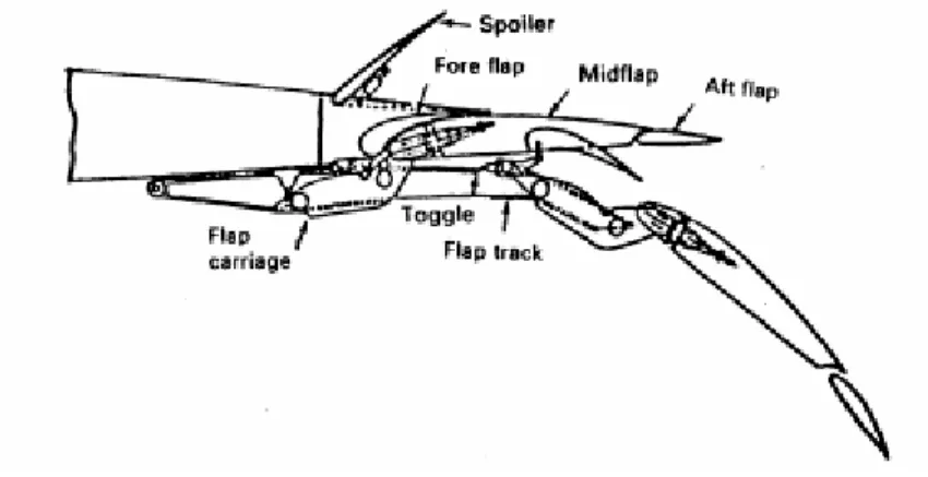
This trend towards more complicated devices saw a fast transition from split flap (as on the Douglas DC3, 1935) to the first double-slotted flap on the Douglas A-26 (Figure 2-5, 1945), and was further boosted by swept wings, which appeared shortly after WWII to address compressibility phenomena, but had detrimental effects on high-lift system effectiveness. Finally, complexity reached a peak on the Boeing 747, with Krueger flap at the leading edge (with variable camber on intermediate sections, Figure 2-30) and triple slotted fowler flap at the trailing edge.

Figure 2-5 Double slotted flap on Douglas A-26 (16)

Since then research has focused on improved simpler systems (Figure 2-6) which reduce weights and costs, while retaining the same performance of previous configurations.

(19)

Figure 2-6 Civil aircraft high lift system complexity trends(23) (data from ref. 11)

2.2 Design Requirements for High Lift Systems

The main objectives of the high-lift system design are:

1. Meeting field length requirements for takeoff and landing 2. Keeping approach speed below reasonable limits for safety 3. Having sufficient climb gradient

2.2.1 Takeoff

A commercial airliner must have a lift-off speed VLOF equal or greater than 1.1 times VMU,

where VMU is the minimum speed allowing the aircraft to safely take off with one engine

inoperative. A lower VMU (achieved through a higher CLmax) is sought, as it means a shorter

take-off length, but there are geometrical constraints, such as fuselage upsw eep angle, which limit ground rotation at take-off and could be a critical issue for derivative aircraft with stretched fuselage (the Airbus A321 is an example (14)).

(20)

After lift-off and landing gear retraction, a safe climb speed V2 greater than 1.2 times VSdyn

(dynamic stall speed) must be maintained, while during the subsequent second climb segment, a constant climb rate gradient of 2.3 (twin-engine aircraft) or 3 (four-engine) is required by FAR and JAR regulations.

Climb gradient γ is 1 −       − = D L W T γ

hence a trade-off between CLmax and L/D, which are conflicting features, must be achieved.

In Figure 2-7 a CL-α curve for three flap settings is shown along with the ground rotation

limit (αlimit). The setting named TO III (higher flap deflection) is better for ground roll (lower

VMU and shorter take-off run), but in Figure 2-8 it is clearly seen that it implies a low L/D

ratio and probably will not meet the climb gradient requirement.

(21)

Figure 2-8 Efficiency at several Take-Off configurations (11)

2.2.2 Landing

Landing condition is deemed the most critical for high-lift system performances on modern turbofan-equipped aircraft, as a low approach speed is sought for safety and economic considerations (Vapproach or V3 must be greater than 1.3 times VSmin). Moreover, cockpit

visibility requirements demand a limit on angle of attack. Figure 2-9 shows a typical situation, where a single slotted flap is unable to provide the CLappr at a reasonable attitude,

(22)

Figure 2-9 CL-α curve changes with several high-lift devices deployment (11)

2.3 Flow Physics of High Lift

The flow around a wing in high-lift configuration is extremely complex as it involves distinct flow regimes cohabiting and different phenomena interacting. Viscous and compressibility effects cannot be neglected as they can control stall in landing and take-off configurations respectively (17).

In the following a brief description of major flow phenomena governing high lift aerodynamics is given.

(23)

2.3.1 Smith’s Analysis of Slotted Aerofoil Aerodynamics

Smith identified five effects governing the aerodynamics of multi-element slotted aerofoils and improving their high-lift behaviour through separation avoidance. He examined mainly the outer inviscid flow and how its changes affect the boundary layer. It must be noted that, although distinction is often made between slat, flap and the main aerofoil, these concepts are general and can apply to generic upstream and downstream elements as well. It must also be stressed that these principles are valid only in the presence of slots or gaps and do not apply to plain flaps and droop-nose devices.

Slat Effect

The circulation of the slat (substituted by a vortex in Figure 2-10) induces a velocity on the leading edge of the main aerofoil opposed to the prevalent flow in that zone. The main effect is a reduction of the local speed on the main element upper side and consequently of the suction peak.

(24)

Figure 2-10 Slat effect (adapted from ref. 18)

An alternative explanation of the phenomenon is that the angle of attack of the main aerofoil is lowered near the aerofoil nose; the flow is thus allowed to make a less sharp turn around the leading edge with less acceleration and suction.

This lowered peak implies that the boundary layer has a lower pressure gradient to stand up to the trailing edge, and therefore stays attached up to higher angles of attack. The CL-α

(25)

Figure 2-11 CL-α curve changes with slat and flap deployment (19)

Circulation Effect

The upwash exerted by a flap on the main aerofoil causes the total lift of the upstream element to increase (Figure 2-12) but the suction peak at the leading edge is increased as well, leading to higher lift for same angle of attack but also lower stall angle as shown in Figure 2-11.

(26)

Dumping Effect

The velocity induced by the downstream element (a flap in Figure 2-13) increases the tangential speed at the trailing edge. The speed at which the flow leaves the element is named “dumping speed” and its higher value is beneficial to boundary layer as it has to stand a lower pressure gradient.

Figure 2-13 Dumping effect on an airfoil-flap configuration (adapted from ref. 18)

Figure 2-14 shows the phenomenon on a slat/main aerofoil configuration: the slat dumping speed is nearly three times as high as the main aerofoil one, and exemplifies why slats can be so highly loaded before stalling.

(27)

Off-the-Surface Pressure Recovery

The boundary layer continues recovery even after leaving the trailing edge, as it undergoes a pressure field similar to the downstream surface one, but the pressure rise does not take place in contact with a wall allowing higher decelerations in shorter lengths.

Fresh Boundary Layer Effect

Subdividing the aerofoil in two or more segments allows on each of them thinner boundary layers which separate at higher angles of attack.

2.3.2 Viscous Effects

(28)

Laminar Bubbles

A laminar bubble is likely to appear on the slat at lower Reynolds numbers, possibly induced by a shock, and may govern the stall particularly at take -off, where the forward element is the most loaded and the first to separate.

A second laminar bubble may be found on the main element and may accentuate the separation tendency at the main element trailing edge.

Confluent Boundary Layers

Wakes of upstream elements may merge with downstream boundary layers and cause an overall lift loss. Although systems optimised for maximum lift exhibit unmerged boundary layers up to the flap trailing edge, in practice merging of slat/main aerofoil wakes upstream of the flap shroud is often difficult to avoid.

Viscous Wake Interaction

The displacement effect of the wake leaving the main element tends to suppress the pressure on the flap; the suction at the start of the recovery is consequently reduced and the boundary layer on the flap has a lower pressure gradient to stand. Thicker wakes (as may be encountered at lower Reynolds numbers or higher incidences) mean higher displacements and are therefore a positive feature ( Figure 2-16); it explains why a reattachment is often observed on flaps at higher angles of attack, whereas the flow is separated at a lower incidence as in curve B of Figure 2-17 compared with curve A (flow attached at lower incidence with higher lift but premature separation).

(29)

Figure 2-16 Viscous wake interaction (adapted from ref. 13)

Figure 2-17 Cl-α for several flow separation situation (from ref. 20)

Relaminarization/Attachment Line Transition

Even with a turbulent attachment line, the flow may become laminar while passing from the lower side to the upper one (Figure 2-15), due to the favourable pressure gradient at the leading edge. A laminar boundary layer is a positive feature up to the point of maximum

(30)

suction, as it allows the subsequent turbulent flow to be thinner at the beginning of recovery and therefore to stand higher pressure gradients.

2.3.3 3D Phenomena (conventional aircraft)

Wing stalling is usually addressed in a quasi-2D fashion (Figure 2-18), by checking wing sections exhibiting the highest section lift coefficient compared to local CLmax. CLmax may

vary spanwise due to different aerofoil families employed at root and tip, and sometimes also due to different local Reynolds number (changing because of taper).

Figure 2-18 Separation detection on wings (from ref. 19)

But care should be given also to truly 3D phenomena, as vortex flows originating at engine nacelle(s) and at wing/fuselage junction (Figure 2-19), since stall is often due to them rather than to conventional 2D separation at maximum local CLmax.

(31)

Pylon-nacelle-wing interaction

Current airliners employs nacelles close-coupled to the wing often implying a slat cut-out which could significantly lower CLmax due to local separation (Figure 2-20middle).

Figure 2-20 Nacelle-wing interaction (20)

This drawback can be “naturally” circumvented by proper control of nacelle vortex flow; these high incidence vortices shed at nacelle sides (Figure 2-20 bottom) tend to reduce local angle of attack and separation on critical zones through their downwash component with beneficial effects on CLmax (Figure 2-21).

(32)

Figure 2-21 Nacelle effects on CL-α curve (20)

Further control is achieved by fixing shedding locations (and therefore shaping vortex flow) with strakes (Figure 2-22) with dramatic reduction of separated flow (Figure 2-23).

(33)

Figure 2-22 Nacelle strake vortex flow (20)

(34)

Slat End/Fuselage Side Problem Area

Another major source of separation is at the wing/fuselage junction. Proper shaping of slat end seems to tackle the problem (Figure 2-24).

(35)

(36)

Stability and Control Issues

High lift system may affect st ability and control as well: Figure 2-25 shows how an incorrectly rigged flap causes separation on the inboard flap starting a chain of event s which degrades lateral trim.

Figure 2-25 Effect of flap separation on lateral trim (22)

How these vortices might interact with the back wing in a prandtlplane configuration is a quite interesting issue deserving further investigation.

2.4 Review of “State-of-the-Art” on Conventional Configurations

Contemporary tendency in high-lift design is towards simpler and lighter systems due to the following advantages(11):

(37)

• Reduction in aerodynamic noise and engine noise due to lower power settings

The reduction in complexity also allow lower costs in:

• Manufacturing

• Maintenance

• Spare parts logistics

This trend is exemplified by the Airbus family in fig. Figure 2-26 and Figure 2-27, where the trailing edge system has evolved from double slotted (fowler) to single slotted (fowler) and the leading edge from slat to droop-nose (on the inboard wing, which stalls first). It must be noticed that, from A320 onwards, thrust-gate is dropped in favour of a continuous trailing edge. A similar tendency is seen on Boeing airplanes, from triple slotted flap on the 727 (Figure 2-28) to single slotted on the 767 (Figure 2-29), and from leading edge Krüger flap on the 747 (Figure 2-30) to three-position slat on the 777 (Figure 2-31).

(38)

Figure 2-27 High-lift devices on Airbus A380

(39)

Figure 2-29 Single slotted Fowler flap on the Boeing B767 (11)

Figure 2-30 Krüger flap on the Boeing B747

(40)

3 Preliminary Design of the High-Lift System for a

Prandtlplane Aircraft

An investigation about preliminary sizing of the high-lift system for a the PP-250 Prandtlplane aircraft has been carried out by calculating the related requirements, choosing the planform layout and checking whether its performances are adequate.

3.1 Requirements Prediction through Several Methods

Several semi-empirical methods, relying basically on statistical data, have been employed with inputs from Table 3-1 in order to find design requirements for low-speed flight; the main aim was to identify the most demanding conditions for CLMAX which will eventually drive the choice of high-lift system features and its complexity.

WT O 208804 kg

Takeoff Runway Length LT O 6000 nm

Range 3000 m (˜ 9900 ft) Take-off Airport Altitude 0 m (sea level) Landing Runway Length LLAND 2000 m

Approach Speed V3 140 kts Cruise Altitude 10500 m 0.254 575 kg/m2 _{(˜ 90 lb/ft}2₎ CD0 0.0225 SREF 362.6 m2 TO W T       TO S W      

(41)

3.1.1 A note on ”dynamic” and ”1-g” values

In ref.'s 24, 19 and 11 the procedure outputs must be corrected in order to be compared with the values obtained by design methods in par. 3.3 and chapt. 4: in fact, regulations refer to a stalling speed VS which is achieved in a manoeuvre (Figure 3-1), while

aerodynamic prediction methods refer to a steady "1 -g" situation (the one usually encountered in a wind tunnel).

Figure 3-1 Time-History of a Typical Stall Manoeuvre (from ref. 19)

A suitable correction factor must therefore be identified and used to transform dynamic data into static ones. Torenbeek suggests, citing BCAR requirements, that VSdyn may be taken

less or equal to 0.94 times VS1-g, and latest issues of JAR regulations (25) implicitly

acknowledge the same value1 thus CLMAX's calculated in the following have been corrected,

where necessary, according to eq. (3.1)

(

)

1 2 0.94 MAX G MAXdyn L L C C − = (3.1) 1

(42)

3.1.2 Raymer's Method

This method (24) focuses on a statistical correlation between the Balanced Field Length (BFL) and the Take Off Parameter (TOP) defined in (3.2).

TO L TO TO C W T S W TOP             = σ (3.2)

Figure 3-2 TOP chart, with PP-250 entry (red line)

Take-off Runway Length is substituted to BFL and the related TOP (Figure 3-2) gives the CLTO required at take-off. From this value, which is related to a take-off speed VTO=1.1VS,

(43)

( )

2

1.1

MAXTOdyn TO

L L

C = C (3.3)

A further check is carried out on Landing distance through (3.4), to verify whether the

CLMAXTO is adequate to meet also landing requirements or a higher value is needed.

305 5 . 0 ₊       ⋅ ⋅ = LAND L LAND S W C L MAX σ (3.4) 3.1.3 Torenbeek's Method

This method, adapted from ref. (19), relies on statistical data as well, and uses equation (3.5) (for take-off) and (3.6) (landing) which resemble a more detailed version of the ones in 3.1.2.

(

)

2 2 1 1.159 1 2.3 ' 2.7 TO TO L TO TO TO S L W gC h S _T W γ σ ρ µ −  _ _∆ _   _ − _⋅ + ∆      ₌   ₋       _ _{ }  _ − +     __{ } _    (3.5) hTO = 10.7m obstacle height

µ’ = 0.01CL_{MAXT O}+ 0.02 equivalent friction coefficient ?ST = 200m inertia distance

??2 = ?2-?2min climb gradient margin

?2min= 0.024 minimum gradient (from Regulations) 2 2 2 V D TO L C T W C γ = _{ } −

  actual climb gradient

2 0 2 2 V L D D C C C AR e π = + ⋅ ⋅

e = 0.7 Oswald’s coefficient in take-off configuration

(

) ( )

2 2 2 0.94 1.2 MAXTO L L C = C lift coefficient at V2 0.85 10 1.52 1.69 / MAX LAND L LAND

TO LAND LAND LAND

h gC L W W S S f h a g ρ       ⋅_ _ =_ _ =_ − _⋅ ⋅     _ _ ₊ (3.6)

(44)

LAND

5

f =

3 landing field length factor hLAND= 15.3 ”screen” height

a = 0.6g average deceleration during landing

Notice that in eq. (3.6) the landing weight is taken as 0.85 times ta ke-off weight, as suggested by ref. (25) for structural analysis.

Figure 3-3 dashed lines refer to take-off requirements, solid lines to landing, the circle is PP-250 design point at take-off

Figure 3-3 is essentially a picture of the design space for

TO W T       _, TO W S       variables. The

(45)

actual aircraft design point (the circle in Figure 3-3). On this basis, it can be seen that the most demanding CLMAX is at landing with a figure of less than 1.9

3.1.4 Method devised from NASA CR 4746

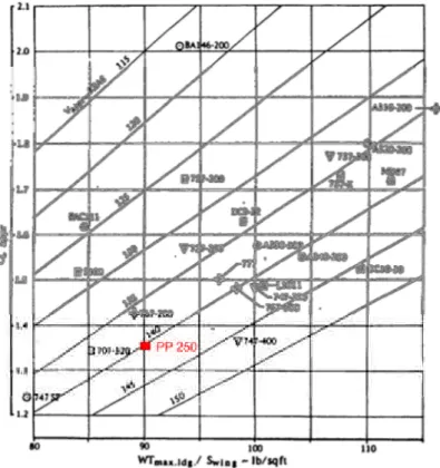
Ref. (14) suggests that high-lift system complexity is usually governed by landing maximum lift requirements, while Rudolph in NASA CR 4746 (11) identifies the approach speed V3 as

the crucial parameter in this situation. It seems therefore reasonable to assume that CL MAX

can be derived by choosing an approach speed and then applying regulation limits in order to find the related stalling speed.

Figure 3-4 Approach Chart adapted from ref. 11- red square is Prandtlplane landing condition

A 140 kts approach speed has been selected as Figure 3-4 shows that airplanes in the same class as the PP-250 exhibit figures between 135 and 145 kts. From this the and the

(46)

CLMAX1-g are subsequently derived with eqs. (3.7) and (3.8). It should also be noticed that

commercial airliner are sized for an approach weight close to 0.75 times WTO.

3 1.3 Sdyn V = ⋅V (3.7)

(

) ( )

1 2 2 0.94 1.3 MAX g approach L L C C − = ⋅ (3.8)

3.1.5 Definitive requirement definition

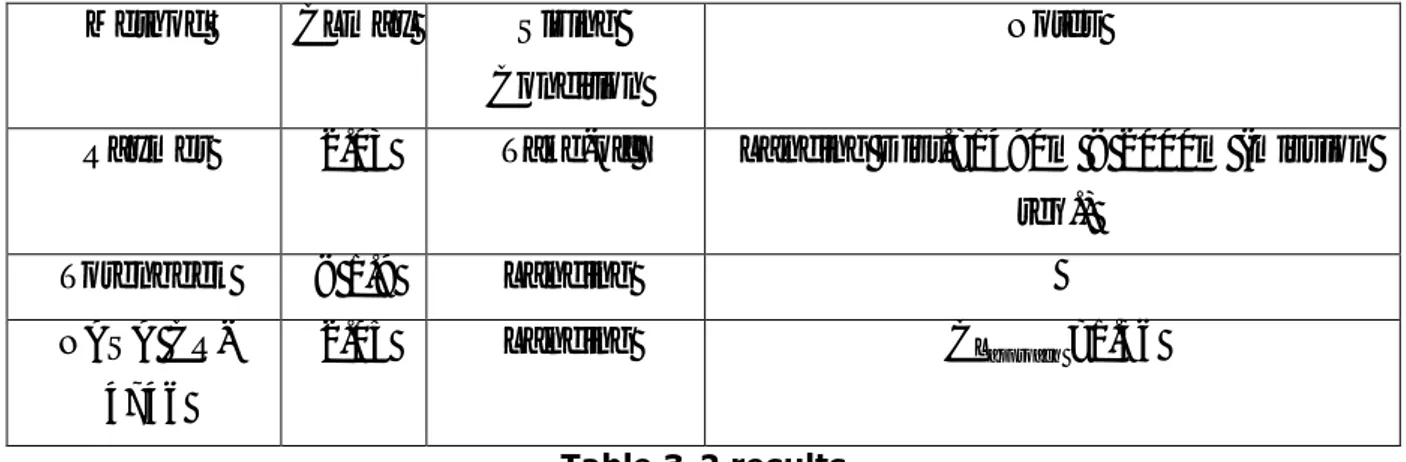
Table shows the CL MAX's found from the previous methods. It should be noticed that values

agree well but are quite different from the usual ones (see for example Figure 4 of ref. 14, where figures are usually greater than 2.5); this is due to the reference area which is comprised of all lifting surfaces in the Prandtlplane, whereas on a conventional aircraft it neglects the tailplane.

Method CLmax Sizing Condition

Notes

Raymer 2.03 Take-off Landing Dist.=1490m < 2000m (mission req.) Torenbeek < 1.9 Landing NASA CR-4746 2.05 Landing CLapproach =1.36 Table 3-2 results

The sizing CL MAX (the highest one) is 2.05 and corresponds, as expected, to a landing

condition.

3.2 High Lift System Layout

(47)

(26) and described in par. 3.2.1, has been taken as a starting point and adapted to the present case.

3.2.1 PP-600 Layout

The PP-600 (Figure 3-5) features a combination of double and single slotted fowler flap on both wings to meet a demanding CL MAX requirement of around 2.5, while elevators are

placed at the inboard sections; these latter devices (which, among their capabilities, have the possibility of being scheduled in conjunction to give a direct lift or pure moment output) have been extensively analyzed in ref. (26).and are credited with providing an adequate longitudinal control power. Ailerons, lastly, are positioned at the outboard of the rear wing in order to keep them effective also in a stall, as wing tip is the last part to separate on forward swept wing.

Figure 3-5 Control and High-Lift Surface Layout on PP-600(26) - 1,5 elevator 2,3,6,7 double-slotted flap 4 single-slotted flap 8 aileron

(48)

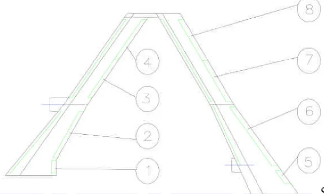
3.2.2 PP-250 Layout

The PP-250 high-lift and control system (Figure 3-6) is based mainly on PP-600 with some notable modifications. The elevators configuration has been retained without changes, as it is deemed effective in ref. (26), whereas the aileron span has been slightly increased up to 0.27% of the total wingspan. Since the CLMAX requirement is considerably lower than the

PP-600 one (2.05 against 2.5 ), the high-lift system has been extensively simplified with single-slotted fowler flap on both wings. Inboard front wing slat has been also retained and a similar device has been ad ded in front of rear wing elevator; their task, apart from increasing overall CLMAX, is to protect elevator from local separation and thus keep them

effective up to higher angles of attack. The front wing would also feature a thrust-gate on the kink with a wing mounted engine (this gap avoids drag caused by interference between engine jet and flaps ,but also lowers flap effectiveness); in the case of rear mounted engines it is obviously not necessary.

(49)

Figure 3-6 Control and High-Lift Surface Layout on PP-250

3.3 Preliminary Analysis

In order to have a first extimate of the aircraft low-speed performances, a semi-empirical method on has been developed, validated against experimental data and applied to the prandtplane configuration under scrutiny.

(50)

The method is mainly based on appendix G of ref. 19, with some minor elements taken from (24). The aim is to obtain a CL-α curve of the aircraft in high-lift configuration starting

from aerofoil data in Table 3-3.

Wing Station Aerofoil Twist [deg] ClMAX2 a0 [deg] Cla [1/rad]

1 NASA SC 20714 +2 2 -5 6.28 2 NASA SC 20714 +1.8 2 -5 6.28 3 Grumman K-2 +4 2 -1.32 6.28 4 Grumman K-2 0 2 -1.32 6.28 5 Grumman K-2 +1.6 2 -1.32 6.28 6 NASA SC 20412 +1.6 2 -5 6.28 7 Grumman K-2 0 2 -1.32 6.28

Table 3-3 Aerofoils on PP-250 wing Corresponding stations shown in Figure 3-7

Figure 3-7 Wing stations (ref. 10)

2D characteristics are converted to 3D through eq. (3.9) and (3.10), where AR is wing aspect ratio, ß is compressibility correction factor, k is an effectiveness factor, ?.5c and ?.25c

(51)

multiplied by 0.9 to allow for spanwise variation of local CL, which causes the wing to stall at

a lower angle of attack (when first section stalls).

2 2 2 2 .5 2 2 tan 1 4 unflapped L L c C AR C AR k α α β β =       +  _ _Λ _  + +  _ _   _ _    (3.9) .25 0.9 cos

MAXunflapped MAX

L l c C = ⋅C ⋅ Λ (3.10)

(

2

)

1 M β = − (3.11) 2 L _M C k α π = (3.12)

Results are then modified for upwash and downwash effects with eq. (3.13) and eq. (3.14), where ? is the taper ratio of the wing subject to downwash, and m and r are its vertical and horizontal distance from the inducing lifting surface (the front wing in this case).

0.18 ε α ∂ = − ∂ (upwash) (3.13)

(

)

4 1.75 1 AR m r ε α π λ ∂ = ∂ ⋅ ⋅ + ⋅ (downwash) (3.14)

Final lift for each ”clean” wing is:

0 1 L L unflapped C C α αε α α  ∂   = ⋅__ − _⋅ − _ ∂    (3.15)

(52)

Next step is taking into account flap and slat contribution to lift (? CLMAX, ? CL0 and ? CLα

integrating them into the following expressions, where Si is the percentage of wing area

influenced by the i-th high-lift device (see Figure 3-8).

.25

0.9 cos

MAX MAXunflapped MAXi i

i L L l c i ref S C C C S   = + ⋅ ∆ ⋅_ _⋅ Λ  

∑

(3.16) 0 0unflapped 0.9 0i cos .25i i L L l c i ref S C C C S   = + ⋅ ∆ ⋅_ _⋅ Λ  

∑

(3.17) unflapped i i L L l i ref S C C C S α α α    = ⋅ ∆ ⋅_ _  _ _ 

∑

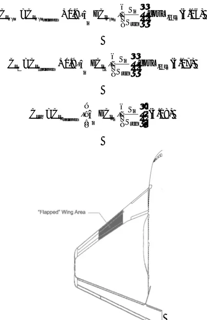
(3.18)

Figure 3-8 An example of ”flapped” wing area, in this case under the influence of the inboard trailing edge flap

(53)

/ 2 flap L f coeff C b AR b ε ⋅∆ ∆ =       (3.19) from ref. [15]

The final extimate for aircraft lift is done with eq.'s (3.20) and (3.21).

total front wing rear wing

L =L ₋ +L ₋ (3.20)

(

)

1

total front wing rear wing

L front wing L rear wing L

ref C S C S C S − − − −   =_ _⋅ ⋅ + ⋅   (3.21) 3.3.2 Validation

A validation must be undertaken in order to check precision and limits of the method applied. Two cases have been analyzed: the first, a swept wing tested at NACA (Figure 3-9, ref. (28)), has been used to examine generic CLα and CLMAX prevision capabilities on

flapped configurations, whereas the second, taken from CFD results of ref. 10, constitutes the only set of data available for a Prandtlplane aircraft of comparable size.

(54)

Figure 3-9 Geometry of configuration tested in NACA TN 3040(28)

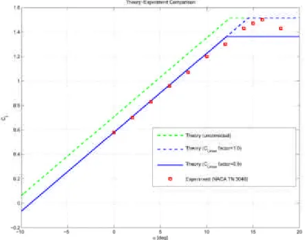
Figure 3-10 Semi-empirical Method Validation against Experimental Data from ref. (28)

(55)

As shown in Figure 3-10, the method predict quite well CLα trend and CLMAX numerical value

which does not seem to need the 0.9 factor (which has been retained anyway for the sake of safety), but lacks precision on the CL0. The latter has been corrected accordingly (blue line) and the method outcome for the second case ( Figure 3-11) is satisfactory. This correction has been extended to the later analysis of section 3.3.3.

Figure 3-11 Validation through CFD output for cruise configuration (CFD data from (10))

3.3.3 Results concerning the Prandtlplane Aircraft

Next step in high-lift system performance prediction is to examine several flap settings so as to gain a better understanding of maximum lift behaviour, and to find the most suitable schedule.

(56)

Figure 3-12 shows that wings alone (with no high -lift devices) do not meet t he requirements, as it could have been expected since the "clean" wing is optimized for cruise. It must be underlined that the aircraft is considered to stall when just one wing stalls.

Figure 3-12 Lift for clean configuration

Configuration df front [deg] df rear [deg] da [deg] CL MAX front CL MAX rear CL MAX total

A 35 35 0 2.2024 2.4701 2.1794

B 35 35 9 2.2024 2.5099 2.2184

C 553 35 0 2.2623 2.4701 2.1390

D 552 552 0 2.2623 2.5650 2.2321

E 35 552 9 2.2623 2.6048 2.2711

Table 3-4 CLMAX results for several flap settings (slat deflection is 23° for all configurations)

(57)

A configuration featuring single slotted fowler flap at their maximum allowable deflection of 35° (configuration A) has been found adequate and provides a maximum lift in excess of 2.15 (Figure 3-13). Notice that the system adopted (single slotted fowler flap) is simpler than the common standard for this class of aircraft, as Boeing 767 and 777 feature a mix of single and double slotted, and Airbus A330-340 whose highly optimized low-speed wing has single slotted flaps but no thrust-gate; the better performance of the Prandtlplane is due to the fact that both lifting surfaces lift upwards, whereas a conventional aircraft features downforce on the tailplane in many flight conditions. It must be stressed also that the semiempirical model relies on rather old data ('60s and '70s, when double and triple slotted high-lift systems were the standard on commerci al airliners), which allow to think that further improvements could be obtained on an optimized Prandtlplane configuration.

(58)

Notice also the strong downwash of front wing flap, which lowers rear wing lift and therefore maximum lift too. This effect is shown more dramatically on configuration C (Figure 3-14), where a 55° deflection of double slotted fowler flaps on front wing causes the overall CLMAX

to decrease to an even lower value than the less flapped configuration A (see Table 3-4).

Figure 3-14 Lift for low-speed wings, configuration C

Figure 3-15 shows performance achieved by Configuration A compared to requirements, and also that the approach angle of attack is slightly greater than 5°, meaning that a further check on cockpit visibility should be carried out (11).

(59)

Figure 3-15 Achieved lift (Configuration A) compared to requirements

Further configurations have been analyzed, and it can be seen that configuration D (Figure 3-16), with double slotted flaps on both wings, would meet also a very stringent requirement on aircraft approach attitude with less than 5° (Figure 3-17).

(60)

Figure 3-17 Lift and attitude requirements, configuration D

From these preliminary results, a few warnings and design guidelines can be inferred:

• As we deal with two lifting surfaces in a non-linear aerodynamic range, we cannot simply do a weighted sum of each wing's lift; we must instead check the situation at every angle of attack

• The first wing to stall causes the entire configuration to stall

• Interaction between the lifting surface must be carefully watched

• The front wing must stall first by reason of stability (the rear one would provide a righting moment improving stall recovery (29))

• The high-lift contribution must be carefully divided between the wings:

o the difference in CLMAX between the wings must be kept to a minimum margin

of safety for stability, as it is useless to have a wing lifting up to higher angles of attack when the other one has already stalled (this situation would mean

(61)

o increasing front wing high-lift contribution could be counterproductive due to the additional downwash; see Configuration C, which paradoxically exhibit lower performances with higher system complexity (double slotted flap) and greater deflection angles

An attempt to define a procedure to design a high-lift system for prandtlplane with wings of comparable size could be as follows:

• size front wing system for a CLMAX slightly greater than aircraft requirement

• size rear wing system so that it achieves a CLMAX slightly greater than the front one,

and at a higher angle of attack (astall-rear> astall-front)

• make provision for a high ? CL0 on the rear wing, as it will pull upwards the total lift

(62)

4 Final Aerodynamic Design of the High Lift System

4.1 Design Procedure

At this stage the need for a procedure to design and analyze wings in details at low speed has arisen. It should enable the engineer to rapidly evaluate different configurations and how changes affect their performances. A Navier-Stokes analysis of the wing is still not viable at this preliminary phase as it requires huge computational facilities and has a low turnaround time. A simplified and effective one has been proposed by Brune and McMasters in ref. 21. It decouples viscous effects from phenomena which are instead more easily caught by potential codes [31].

The first step is therefore an inviscid analysis of the Cl span distribution in order to detect

possible critical areas (Figure 4-1). This operation can be aptly done with a panel method, a vortex lattice method or even a lifting line method (but the latter has more difficulties in correctly modelling partial flapped sections), since spanwise lift distribution is largely dominated by potential phenomena.

0 0.2 0.4 0.6 0.8 1 1.2 1.4 0 0.2 0.4 0.6 0.8 1 1.2 eta Cl Cl Cl max Critical Area

(63)

In these areas, where the Cl is higher, corresponding better low-speed performances are

demanded to the airfoil; these performances are embodied by the local available Cl MAX

which varies spanwise because of different local airfoil shape and Reynolds number.

Once these section(s) are identified, a more detailed analysis of their characteristics can be carried out with a Navier-Stokes code (Figure 4-2and Figure 4-3) or an inviscid-viscous interactional code (Figure 4-4).

Figure 4-2 NLR 7301 flapped airfoil (turbulent kinetic energy flowfield) from ref.33

(64)

Figure 4-4 Coupled viscous-inviscid airfoil analysis with XFOIL

Care should be exerted when defining the airfoil to be analyzed: Cl distribution is calculated

for the streamwise airfoil (Figure 4-5), but on a swept wing the flow is really 2D only on the airfoil projected normal to the sweep line (Figure 4-6 and eq. (4.1)).

(65)

Figure 4-6 Streamlines about an infinite yawed wing (from ref. 32)

It is therefore necessary to calculate a new "normal" Cl (eq.(4.3)) and assess its "normal"

performances. The transforming equation are (4.1) to (4.3), where M is Mach number.

( ) cos normal s treamwise c =c ⋅ Λ (4.1) cos normal streamwise M_∞ =M_∞ ⋅ Λ (4.2) 2 1 cos l normal lstreamwise C =C ⋅ Λ (4.3)

4.2 Design Tools

4.2.1 AVL

AVL is a vortex lattice method developed at the MIT Department of Aeronautics and Astronautics (34). It can model an aircraft with thin lifting surfaces and also fuselages, nacelles and general slender bodies with source+doublet segments. It has a large set of output variables, including lift, moment, lift distribution and aerodynamic derivatives. It can perform Trefftz's plane analysis too.

(66)

4.2.2 XFOIL

XFOIL is a program to analyse and design isolated airfoil by mea ns of inviscid panel method (35,36). A boundary layer solver is also available to take viscous effects into account.

4.2.3 Fluent

Fluent is a multi-purpose program able to address a wide range of CFD and heat transfer problems (37). It features a complete set of Turbulence models and is capable of solving compressible and incompressible flows.

4.3 AVL Validation

A validation of the programs (30) is necessary in order to acquire a "sensitivity" (albeit forcefully limited) to the order of magnitude of their outputs and to be able to make a reality check on their results. It is quite impossible to make a "complete" validation of the software in a short time frame, it is therefore better to concentrate on selected topics functional to the context of the present work. For what AVL is concerned, three main issues are to be addressed: its capability to correctly predict lift distribution on lifting surfaces and force and moments on complex configurations, such as a flapped aircraft (with tail) and a Prandtlplane.

These results will be subsequently employed as building blocks to a combination of them: a flapped configuration of a PrandtlPlane aircraft.

4.3.1 Lift and Lift Distribution

(67)

It can be seen in Figure 4-8 that CL prediction are accurate up to separation angle of attack,

and also local Cl distribution is in fairly good agreement with experimental data for even

mildly separated flow (α=8° and α=12° in Figure 4-9 and Figure 4-10 respectively).

CL comparison (slat extracted)

0 0.2 0.4 0.6 0.8 1 1.2 1.4 1.6 0 5 10 15 20 alpha CL CL exp CL AVL

Figure 4-8 CL-α curve for the NACA wing

Cl slat retracted 0 0.2 0.4 0.6 0.8 1 1.2 1.4 1.6 1.8 0 0.2 0.4 0.6 0.8 1 1.2 eta Cl Cl alpha=0 exp Cl alpha=8.4 exp Cl alpha=0 AVL Cl alpha=8.4 AVL

(68)

Cl slat extracted 0 0.2 0.4 0.6 0.8 1 1.2 1.4 1.6 1.8 2 0 0.2 0.4 0.6 0.8 1 1.2 eta Cl Cl alpha=0 exp Cl alpha=12.4 exp Cl alpha=0 AVL Cl alpha=12.4 AVL

Figure 4-10 Cl spanwise distribution (slat retracted)

4.3.2 Lift and Moment data on a Complex Configuration

A validation on a more complex configuration (ref. 38, ) has been carried out so as to check whether AVL is able to assess direct lift and moments on a lifting system including interaction between lifting surface (here wing and tail), fuselage effect and flap deployment.

(69)

Figure 4-11 Civil aircraft configuration tested in ref.38

Figure 4-12 Angle Nomenclature

The configuration has been modelled with and without the source-doublet fuselage (Figure 4-13, Figure 4-14, Figure 4-19, Figure 4-20), for mid and low tail position (see Figure 4-11) and taiplane setting it =2.6° and it =2.2° (see Figure 4-12 for reference angles). Results for

(70)

the first tail position are shown in Figure 4-15 to Figure 4-18, and in Figure 4-21 to Figure 4-24 for the second one. Flap effects (available only for the second configuration) are shown in Figure 4-25 to Figure 4-28 and the static margin variation due to flap deployment is shown in Figure 4-29. Results are summarized in Table 4-1.

(71)

-0.6 -0.4 -0.2 0 0.2 0.4 0.6 0.8 1 1.2 1.4 -5 0 5 10 15 alpha CL CL exp CL AVL CL AVL no fuselage

Figure 4-15 Mid tail, it=2.6°

-0.7 -0.6 -0.5 -0.4 -0.3 -0.2 -0.1 0 0.1 0.2 0.3 -5 0 5 10 15 alpha Cm Cm exp Cm AVL Cm AVL no fuselage

(72)

-0.7 -0.6 -0.5 -0.4 -0.3 -0.2 -0.1 0 0.1 0.2 0.3 -0.5 0 0.5 1 1.5 CL Cm Cm exp Cm AVL Cm AVL no fuselage

Figure 4-17 Mid tail, it=2.6°

-0.8 -0.7 -0.6 -0.5 -0.4 -0.3 -0.2 -0.1 0 -5 0 5 10 15 alpha s tatic margin

static margin exp static margin AVL no fus static margin AVL

(73)

Figure 4-19 Aircraft model with doublet-source fuselage, low tail

(74)

-0.6 -0.4 -0.2 0 0.2 0.4 0.6 0.8 1 1.2 1.4 -5 0 5 10 15 20 alpha CL CL exp CL AVL CL AVL no fuselage

Figure 4-21 Low tail, it=2.2°

-0.6 -0.5 -0.4 -0.3 -0.2 -0.1 0 0.1 0.2 0.3 -5 0 5 10 15 alpha Cm Cm exp Cm AVL Cm AVL no fuselage

(75)

-0.6 -0.4 -0.2 0 0.2 0.4 -0.5 0 0.5 1 1.5 CL Cm Cm exp Cm AVL Cm AVL no fuselage

-0.7 -0.6 -0.5 -0.4 -0.3 -0.2 -0.1 0 -5 0 5 10 15 20 alpha static margin

static margin exp static margin AVL static margin AVL no fus

0 0.5 1 1.5 2 2.5 -5 0 5 10 15 20 alpha CL CL exp CL AVL CL AVL no fuselage

(76)

-0.7 -0.6 -0.5 -0.4 -0.3 -0.2 -0.1 0 0.1 0.2 -5 0 5 10 15 20 alpha Cm Cm exp Cm AVL Cm AVL no fuselage

Figure 4-26 low tail it=2.2 deg, flapped

-0.7 -0.6 -0.5 -0.4 -0.3 -0.2 -0.1 0 0.1 0.2 0 0.5 1 1.5 2 2.5 CL Cm Cm exp Cm AVL Cm AVL no fuselage

(77)

-0.8 -0.7 -0.6 -0.5 -0.4 -0.3 -0.2 -0.1 0 -5 0 5 10 15 alpha static margin

static margin exp

static margin average from Cm-CL curves

static margin AVL no fus

Figure 4-28 low tail it=2.2 deg, flapped

Delta%>0 corresponds to a decrease in stability

-5 0 5 10 15 20 25 30 35 -4 -2 0 2 4 6 8 10 12 14 alpha

Delta% static margin

exp

AVL averaged AVL no fus

(78)

AVL with Doublet Fuselage AVL - Lifting Surfaces only L C α Overpredicted by as high as 40% (unreliable) Difference is less than 10% (higher than experiment) 0 α 1 to 3 degree greater than experimental value 0÷3° lower than experiment m C α Unreliable (too low) Twice the experiment datum (unreliable) TRIM α Difference greater than 2°, unreliable 0÷2° greater than experiment

Static Margin Lower than experiment, on the verge of instability Higher than experiment (nearly twice, coherent with m C αdata) ∆Static Margin due to flap deflection Predicts nearly no variation compared to an experimental 10% decrease of stability Predicts nearly no variation compared to an experimental 10% decrease of stability

Table 4-1 AVL Output Compared to Experiment

The following conclusions can be inferred: The doublet fuselage model tends overpredict lift and underpredict stability, therefore performs rather bad and should be excluded.

The model without doublet fuselage assesses lift and αTRIM rather well, but the CM-α curve

is not as good (more stable than experiment). Variation in static margin is minimal in the experimental case (5-15% less stable), whereas for AVL it is nearly zero (at low angles of attacks it is anyway in the right verse (less stable)).

Fuselage effect has the same order of magnitude of the tail, but the doublet fuselage has a stronger unrealistic contribution.

(79)

4.3.3 Lift and Moment data on a Prandtlplane configuration (CFD data)

Comparison with PrandtPlane data can be done only relative to CFD data. The complete configuration has been analysed at high (Figure 4-31) and low speed (Figure 4-30). The PrandtlPlane exhibits the usual variations due to shockwaves (see Figure 4-31, where they are highlighted with density gradient, obtaining a pseudo-Schlieren visualization) in lift an stability data (at transonic speed the aircraft is more stable and shows a higher CLα

derivative).

(80)

Figure 4-31PP250 at M=0.85

The two familiar models (with and without fuselage) are employed in this case too (Figure 4-32 and Figure 4-33), and results of Figure 4-34 to Figure 4-36 are summarized as usual in Table 4-2.

(81)

Figure 4-33 PrandtlPlane – lifting surfaces only 0 0.1 0.2 0.3 0.4 0.5 0.6 0 0.5 1 1.5 2 2.5 alpha CL CL Fluent Euler M=0.85 CL Fluent Euler M=0 CL AVL M=0 CL AVL no fus M=0

(82)

-0.05 0 0.05 0.1 0.15 0.2 0 0.5 1 1.5 2 2.5 alpha Cm Cm_CG Fluent Euler M=0.85 Cm_CG Fluent Euler M=0 Cm_CG AVL M=0 Cm_CG AVL no fus M=0

Figure 4-35 PrandtlPlane CM-α curve

-4 -3.5 -3 -2.5 -2 -1.5 -1 -0.5 0 0.5 1 0 0.2 0.4 0.6 0.8 1 1.2 alpha [deg]

Dimensional Static Margin [m]

Dimensional Static Margin Fluent M=0.85

Dimensional Static Margin Fluent M=0

Dimensional Static Margin AVL [m]

Dimensional Static Margin AVL no fus [m]

(83)

AVL with Doublet Fuselage AVL - Lifting Surfaces only L C α AVL value 15% lower than Fluent Euler data 0 α 2.5 degrees lower than Fluent Euler data m C α Values are actually coincident (difference below 2%) TRIM α 2.3 degrees lower than Fluent Euler data

Static Margin Not stable (doublets overestimate fuselage influence) 20% more stable

Table 4-2 AVL Output Compared to Fluent CFD analysis

The doublet fuselage model has been discarded as its stability outputs are highly unreliable.

4.4 X-foil/Fluent Validation

In order to validate the 2D tools, as test-case a supercritical airfoil (ref.39, Figure 4-37) has been selected.

4.4.1 Stall Behaviour of a Supercritical Airfoil

The airfoil has been analyzed in three conditions ( Figure 4-38 to Figure 4-40) with two turbulence model in Fluent (Spalrt-Allmaras and k-ω SST) and with XFOIL.

(84)

Figure 4-37 Supercritical airfoil tested in ref.39 M=0.15 Re=2x10^6 0 0.2 0.4 0.6 0.8 1 1.2 1.4 1.6 1.8 2 0 5 10 15 20 25 alpha Cl exp Xfoil Fluent SA Fluent SST

(85)

M=0.15 Re=9.3x10^6 0 0.5 1 1.5 2 2.5 0 5 10 15 20 25 alpha Cl Xfoil Fluent SA exp

Figure 4-39 Test condition 2

M=0.15 Re=17x10^6 0 0.5 1 1.5 2 2.5 0 5 10 15 20 25 alpha Cl exp Xfoil Fluent SA Fluent SST

(86)

1.4 1.5 1.6 1.7 1.8 1.9 2 2.1 2.2 1.90E+06 Re Cl max exp Xfoil Fluent

Figure 4-41 Reynolds Number trends

The Spalart-Allmaras and k-ω SST model have been chosen as they perform quite well for flows whose separation is due to pressure gradient (41), but the k-ω SST model probably needs accurate settings as it missed Cl MAX value in condition 3. This is probably due to an

overproduction of turbulence in the leading edge region ( Figure 4-42 and Figure 4-43) where the flow is assumed to be laminar instead. This is a typical drawback of the standard k-ε model (Figure 4-44), which the SST is thought to have addressed. The SST model is actually a blending of k-ε and k-ω equations, supposed to switch on each one in the field best suited to its characteristics, but probably in this case it requires a more expert operator.

(87)

Figure 4-42 Spurious turbulence shed by SST model

(88)

Figure 4-44 k-ε spurious turbulence effect (ref.42)

In the end the Spalart-Allmaras model is the first choice, as it enforces a "natural" transition from laminar to turbulent flow and is thus able to detect also the inversion in Re-ClMAX

shown in Figure 4-41.

4.5 Design Procedure Validation

The procedure outlined in par.4.1 must be checked against experiment data to see its ability to correctly predict trends due to design variables changes. The test-case (43) is a swept wing (Figure 4-46) with symmetrical airfoil and no spanwise twist, and its re-designed version (whose intent was to improve stalling characteristics) with a cambered airfoil and washout at the tip (Figure 4-45).

Figure 4-45 Washout (after ref. 44)

More specifically, the validation aims at establishing if the procedure is able to

(89)

Figure 4-46 Dimensions of the two models of ref. 43

The plain wing (Figure 4-47) starts to separate (i.e. to deviate from theoretical attached-flow Cl distribution) roughly at 65% of its semispan and its global CL at separation is about 0.4,

but it exhibits an actual deviation from linear range in the CL-α curve (Figure 4-49) only for a

(90)

Figure 4-47 Cl distribution for the plain wing

The cambered and twisted wing features a separation point more inboard (60% of semispan) and at a higher CL value (CL=0.6). The actual departure from linearity is at

CL=0.8 (Figure 4-49). These discrepancies are probably due to the use of a lifting -line

(91)

Experiment 0 0.2 0.4 0.6 0.8 1 1.2 0 10 20 30 alpha CL

plain wing exp. twisted cambered wing exp.

Figure 4-49 Lift comparison between the wings

The first step in applying the potential-viscous analysis to the same cases is to generate a vortex lattice model of the wing (Figure 4-50) and to calculate Cl MAX for root and tip airfoils

(Figure 4-51 and Figure 4-52).

(92)

Xfoil 0 0.2 0.4 0.6 0.8 1 1.2 1.4 1.6 0 5 10 15 20 alpha Xf oil

Figure 4-51 Cl-α curve for the symmetrical NACA 64-A010 employed at the root

Xfoil 0 0.2 0.4 0.6 0.8 1 1.2 1.4 0 5 10 15 20 alpha Cl Xfoil

Figure 4-52 Cl-α curve for the symmetrical NACA 64-A010 employed at the tip

It is now possible to analyze the separation by drawing a Cl MAX line joining the root and tip

values (Figure 4-53, notice the slight difference between the two geometrically similar airfoil, due to the different local Reynolds numbers). This line is assumed to be a separation threshold for the Cl distribution curve (both values are depicted against non-dimensional

semispanwise coordinate eta): once the latter trespass the former, the section is stalled and the flow starts to separate. It must be noticed that the Cl MAX is not the 2D value represented

(93)

CL = 0.6 0 0.2 0.4 0.6 0.8 0 0.2 0.4 0.6 0.8 1 1.2 eta Cl Cl Clmax

Figure 4-53 Cl distribution for the plain wing at CL=0.6

The comparison between the situation at CL=0.6 (CL is the figure for the whole wing,

opposed to Cl, which is the local one pertaining to the airfoil) and CL=0.7 (Figure 4-54)

leads to the deduction that the flow is separated in the latter case and that this value correlates well with the separation CL of the experimental curve (Figure 4-55), better than

the theoretical results of ref. 43 shown in Figure 4-47 since, as mentioned above, a low-fidelity potential method (Weissinger's lifting line) with slightly poorer performances has been employed in that case.

CL=0.7 0 0.2 0.4 0.6 0.8 1 0 0.2 0.4 0.6 0.8 1 1.2 eta Cl Cl Clmax

(94)

0 0.1 0.2 0.3 0.4 0.5 0.6 0.7 0.8 0.9 1 0 10 20 30 alpha CL

plain wing exp. plain wing - AVL separation - AVL Same separation CL and α

Figure 4-55 Experimental-numerical comparison – plain wing

The same procedure is applied to the twisted and cambered wing ( Figure 4-56 to Figure 4-60). 0 0.2 0.4 0.6 0.8 1 1.2 1.4 1.6 1.8 2 0 5 10 15 20 25 alpha Serie1

(95)

Xfoil 0 0.2 0.4 0.6 0.8 1 1.2 1.4 1.6 1.8 2 0 5 10 15 20 25 alpha Xf oil

Figure 4-57 Cl-α curve for the cambered NACA 64-A810 employed at the tip

Twisted & Cambered Wing - CL = 0.8

0 0.2 0.4 0.6 0.8 1 0 0.2 0.4 0.6 0.8 1 1.2 eta Cl Cl Cl max

(96)

Twisted & Cambered Wing - CL = 0.9 0 0.2 0.4 0.6 0.8 1 1.2 0 0.2 0.4 0.6 0.8 1 1.2 eta Cl Cl Cl max

Figure 4-59 Cl distribution for the twisted and cambered wing at CL=0.9

0 0.2 0.4 0.6 0.8 1 1.2 0 5 10 15 20 25 alpha CL twisted cambered wing exp. twisted cambered wing - AVL separation - AVL Same separation CL

Figure 4-60 Experimental-numerical comparison – twisted and cambered wing

In this case (Figure 4-61) the correlation is only on the CL value, meaning that the α related

to separation is not the correct one. This difference is less important as the designer is concerned more with aircraft maximum lift than the corresponding α.