CIRTEN
Consorzio Interuniversitario per la Ricerca TEcnologica Nucleare
UNIVERSITÀ
POLITECNICO DI TORINO
Advances in the development of the code FRENETIC for the
coupled dynamics of lead-cooled reactors
Autori
Roberto Bonifetto, Dominic Caron, Sandra Dulla, Valerio Mascolino, Piero Ravetto, Laura Savoldi, Domenico Valerio, Roberto Zanino
CERSE-POLITO RL 1572/2015
Indice
Abstract _______________________________________________________ 3
1
Introduction ________________________________________________ 4
2
Description of the EBR-II reactor and of the analyzed transients _____ 5
2.1
The EBR-II reactor _______________________________________ 5
2.2
The Shutdown Heat Removal Tests __________________________ 8
2.2.1 SHRT-17 _______________________________________________________ 9 2.2.2 SHRT-45R _____________________________________________________ 13
3
Development and validation of the thermal-hydraulic module ______ 16
3.1
Implementations in the thermal-hydraulic module ____________ 18
3.1.1 Box-in-the-box model ____________________________________________ 21 3.1.2 Pin radial model ________________________________________________ 23
3.2
Results and discussion ____________________________________ 25
3.2.1 Boundary conditions sets _________________________________________ 26 3.2.2 Box-in-the-box results ____________________________________________ 29 3.2.3 Radial pin model results __________________________________________ 39
3.3
Conclusions ____________________________________________ 44
4
Development of the neutronic module __________________________ 45
4.1
Introduction ____________________________________________ 45
4.2
Decay heat model and methods of solution ___________________ 45
4.3
Representative results ____________________________________ 46
4.4
Conclusions ____________________________________________ 49
5
Preliminary validation of the coupled modules of FRENETIC ______ 49
5.1
Steady state analysis _____________________________________ 50
5.2
Transient results ________________________________________ 53
5.3
Parametric study with the quasi-static method ________________ 55
Abstract
The simulation of the dynamic behavior of lead-cooled fast reactors (LFRs) is a key step in the development of this innovative nuclear technology. To this aim, computational tools for the coupled neutronic/thermal-hydraulic description of the reactor core need to be developed. This task can be carried out at different levels of complication. Some codes are characterized by a highly detailed description of the system components, but they also require a high computational cost.
At Politecnico di Torino, the research group of nuclear engineering is developing the FRENETIC code for the dynamic simulation of LFR cores with closed hexagonal fuel elements at a reduced computational cost, suitable for parametric evaluations and simulations of safety-related transients. The code separately solves the neutronic and thermal-hydraulic model equations, with neutronic/thermal-hydraulic feedback introduced through a coupling procedure. The work carried out during this year activity is focused on the following topics:
further development and validation of the thermal-hydraulic module by introducing additional models for the treatment of hexagonal fuel assemblies of a specific geometry (the so-called "box-in-the-box" configuration) and the radial conduction in the fuel pin; development of the neutronic module by introducing a new decay-heat model;
first coupled neutronic/thermal-hydraulic validation of the code against the shutdown heat removal tests performed on the Experimental Breeder Reactor-II of Argonne National Laboratory.
1 Introduction
Several activities are ongoing in Europe and in particular in Italy around the development of the GenIV lead-cooled fast reactor (LFR) [1]. The main concepts which evolved over the years are those of the ELFR (the first-of-a-kind EU reactor) [2], of ALFRED (the EU demonstrator) [3] and of MYRRHA (the EU technology pilot plant) [4]. Indeed, Ansaldo Nuclear, ENEA and the Institute of Nuclear Research of Romania have signed at the end of December 2013 an agreement for the establishment of the Falcon Consortium (Fostering Alfred Construction), whose objective is to construct ALFRED in Romania.
Within that framework, the FRENETIC (Fast REactor NEutronics/Thermal-hydraulICs) code has been recently developed for the simulation of coupled neutronic/thermal-hydraulic transients in LFRs with the core arranged in hexagonal assemblies (HAs), enclosed in a duct [5]. The code has the ambition to provide fast approximate solutions for core design and/or safety analysis, and this thanks to the fact that the 3D problem is solved with a simplified approach. The neutronic (NE) module in FRENETIC solves the multigroup neutron diffusion equations with delayed neutron precursors using a nodal discretisation in space and a quasi-static discretisation in time. The thermal hydraulic (TH) module of FRENETIC solves the 1D (axial) mass momentum and energy conservations laws of the coolant, together with the 1D (axial) heat conduction equation in the fuel pins, in each assembly. The assemblies are then thermally coupled to each other on each horizontal cross section of the core, resulting in a quasi-3D model.
The work carried out in 2014 continues the development of this computational tool, following the previous steps carried out starting from the year 2011 [5, 6, 7, 8, 9]. The historical progress to the beginning of the period covered by the present report is summarised in Figure 1, while Figure 2 sketches the coupling strategy that has been adopted from the beginning of the project, allowing the possibility to perform separately the development and validation of the NE and TH modules.
Figure 1. Evolution of the modelling capabilities of the FRENETIC code.
Figure 2. Coupling of the FRENETIC thermal-hydraulic and neutronic modules.
further development of the thermal-hydraulic module by introducing additional models for the treatment of hexagonal fuel assemblies of a specific geometry (the so-called "box-in-the-box" configuration) and the radial conduction in the fuel pin, and prosecution of the validation activity [10, 11, 12] using data from the sodium-cooled Experimental Breeder Reactor-II (EBR-II) of Argonne National Laboratory;
development of the neutronic module by introducing a new decay-heat model;
first coupled neutronic/thermal-hydraulic validation of the code against the shutdown heat removal tests performed on the EBR-II.
In order to validate the FRENETIC code and due to the lack of experimental data from lead-cooled reactors, a series of transients regarding the EBR-II (sodium-lead-cooled) reactor were analyzed within the framework of a multi-party benchmarking exercise coordinated by the IAEA [13].
2 Description of the EBR-II reactor and of the analyzed
transients
The following section presents a brief description of the Experimental Breeder Reactor-II (EBR-II) and two of the Shutdown Heat Removal Tests (SHRTs), as these transients are assessed with the FRENETIC code in later sections of this report.
2.1 The EBR-II reactor
During 1944, scientists of the caliber of Fermi, Szilard and Wigner discussed the possibility of using nuclear energy not only for military purposes but also to light their cities [14]. It was not completely clear, at that time, what was the available quantity of fissile material on Earth. This coupled with the need of use as much as possible Uranium to develop atomic bombs, led this team of scientists to think of the possibility of designing a nuclear reactor able to produce more fissile materials than it consumed.
The chain of events led, in the frame of Argonne National Laboratories, to the birth of EBR-I in 1951. This reactor showed the feasibility of the breeding reactor concept and the possibility to control a chain reaction with a fast spectrum reactor with no moderation and sodium as a coolant. The EBR-II was then conceived and the innovative features of the reactor were already clear at that time: the possibility to close the fuel cycle, coupling the reactor with a suitable reprocessing plant; the proliferation resistance of fuel irradiated in fast reactors, due to its very high radioactivity concentration.
The EBR-II reactor was a 62.5 MWth (~20 MWel) pool type sodium cooled reactor: all the
primary components were submerged in the primary tank, containing approximately 340 m3 of sodium [13]. The upper plenum is at the same pressure for the whole reactor, while the inlet plenum is at different pressures with the inner core receiving sodium from the high-pressure plenum (~85 % of the total flow rate) while the outer blanket region received sodium from the low pressure plenum. Hot sodium mixes in the common upper plenum before going to the
Figure 3. EBR-II plant schematic [13].
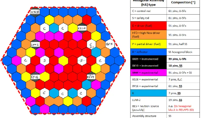
Figure 4. EBR-II reactor pool with HAs (left) and core pattern of the SHRT-45R transient (right) [15].
The core of the EBR-II is composed of 637 hexagonal assemblies (HAs), clearly divided in two zones: the inner core zone in which the fuel elements are present, and the outer core zone composed by reflector and breeding blanket elements. The flow to the inner core HAs, as stated above, is fed by a high-pressure inlet plenum, while the reflector and blanket flows are fed through the low-pressure inlet plenum.
The fuel elements are composed of a metallic alloy of uranium uniquely used for the EBR-II reactor called U-5Fs. U-5Fs is composed 95% (in weight) by metallic uranium and for the remaining 5% by fissium, which is a mixture of alloying elements composed by in 2.4% Mo, 1.9% Ru, 0.3% Rh, 0.2% Pd, 0.1% Zr and 0.01% Nb [16]. The uranium enrichment in the fuel is equal to the 67% weight content of 235U.
All the constructive drawings and compositions of the different types of hexagonal assemblies present inside the reactor are reported in detail in the ANL benchmark specifications [13]. The pin lattice is triangular, as usual for hexagonal assemblies, with no spacer grids: the spacing function is carried out by a spacer wire which, in some instrumented assemblies, also acts as a thermocouple (Figure 5). Only part of the assembly height is active; above and below the fuel region, an axial reflector is present.
Figure 5. Axial view, horizontal section and lattice detail of HA of the BIB type [15].
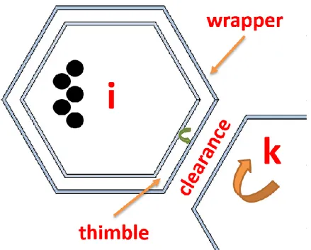
Some of the assemblies have a smaller hexagonal box inside the main one (Figure 6). These assemblies are referred to as the “Box-in-the-box” (BIB) type. In the space between the two stainless steel boxes, referred to as “thimble”, a certain fraction of sodium is flowing.
Figure 6. Schematics of BIB HAs and pre-existing inter-assembly heat transfer model
2.2 The Shutdown Heat Removal Tests
During the time EBR-II operated, a certain number of tests have been conducted in order to prove the inherent safety features of pool-type SFRs. The IAEA benchmark consists in the study of two of these transients in order to develop and improve experience on both neutronic and thermal-hydraulic modeling of transients of major safety concern, to provide both expertise and computational tools for the future GenIV reactors design and safety assessments.
Among these transients are the SHRT-17 and SHRT-45R, where SHRT stands for Shutdown Heat Removal Test. These tests were performed in 1984 and 1986 respectively, and both involved the trip of the pumps, therefore leading the reactor to work under natural circulation conditions, initially supported by the coast down of the immersed sodium pump.
The IAEA benchmark participants studied and modeled the whole reactor system, including pumps, heat exchangers and pipes from both primary and secondary (intermediate) loops (Figure 7).
Figure 7. Benchmark model of primary vessel components, elevation view [13].
During the SHRT tests the reactor was equipped with two experimental HAs (XX09, a fuel assembly; XX10, a dummy assembly). Experimental data from these assemblies were provided for both SHRT after the first blind phase of the benchmark.
For the purposes of the benchmarking activity, the SHRT-17 transient is intended to be a purely thermal-hydraulic study, with the time-dependent power distribution provided as input by ANL. Instead, the SHRT-45R transient treats the time-dependent power distribution as an unknown quantity, requiring the participants to perform coupled neutronic/thermal-hydraulic analyses. Each of the transients is now described in further detail.
2.2.1 SHRT-17
pump was not activated, while normally it would receive power from battery backups during a station blackout. After the start of the test no automatic or operator action took place until the test had concluded.
Data on decay heat power were available from ANL, and the assumption of uniform axial heating was made in making the calculations. ANL provided to participants also the model for pumps behavior in the Benchmark Specifications [13] and the constructor data concerning them, as well as the coastdown curves retrieved by means of this model. Data on pumps experimental flow rates were subsequently released by ANL in the post blind phase, but unfortunately only data for one of the two pumps were actually recorded; this lack of experimental data will impact on the analysis performed here. Coolant and fuel properties libraries were also provided by ANL [13, 17].
In Figure 8, the core-loading pattern for SHRT-17 is reported. A number denotes each hexagonal assembly, fully described in the Benchmark Specifications [13].
Figure 8. SHRT-17 core loading pattern for the first eight rings [13].
Figure 9 shows the power evolution in the first 60 seconds of the transient. The SHRT-17 transient started from an initial equilibrium configuration that was rated at a power of 57.3 MWth
rather than the nominal 62.5 MWth. The complete power distribution was provided by ANL in
tabular form for the entire duration of the transient (900 s). The decay heat power was calculated based on the ANS decay heat standard for Light Water Reactors, because no experimental data are available for EBR-II (neither are they available for SFRs in general).
Figure 9. Power evolution as given by ANL [13].
The initial conditions of the transient were provided as well. Initial (steady state) flow rates have been calculated by ANL by means of the EBRFLOW code. This code was optimized on the EBR-II plant instrument data. Power at time t = 0 s in each HA, instead, was evaluated through the two dimensional discrete ordinates transport code DOT-III, developed by Oak Ridge National Laboratory: this code calculated both neutron and gamma flux distributions within each assembly. These data are reported on the Benchmark Specifications [13] as well.
In Figure 10 the experimental flow rates from primary pumps are reported. These data have been provided by ANL after the first blind phase of the benchmark. As stated before, the flow rate of one of the primary pumps (pump #1) was not registered. Participants to the benchmark used the experimental flow rates from pump #2 to better describe their pumps models and therefore to provide more accurate core inlet flow rates data to the core calculations.
Figure 10. SHRT-17 experimental pump flow rates (post-blind phase) [18].
In addition, experimental results concerning the instrumented assemblies XX09 and XX10 were also provided after the blind phase concluded. These constitute the main reference to evaluate the performances of the participants’ codes with the respect to the analysis of the core region, and therefore the only one of interest for FRENETIC calculations since the core is the only part of the system modeled, see below. The data provided consisted in the measurements coming from the assembly flowmeters and those from thermocouples at different element heights and locations in the hexagon cross section. Figure 11 shows an example of these results, for the temperature at the top of the core measured by the spacer wire thermocouple near the central pin.
Figure 11. SHRT-17 example of experimental data on instrumented assemblies. TTC10 and TTC31 are thermocouple locations in the two assemblies [18].
Post-blind experimental results released by ANL also involved inlet and outlet plena average temperatures and data related to the rest of the primary components, such as the temperature drop across the Intermediate Heat Exchanger (IHX). They are not reported here since they are not used for comparison.
2.2.2 SHRT-45R
The SHRT-45R transient was carried out on April 3, 1986, to demonstrate the effectiveness of passive reactivity feedbacks in the EBR-II (and in all pool-type SFR). The Core Loading pattern, shown in Figure 12, is different from the one of SHRT-17. The Plant Protection System was disabled to avoid the SCRAM. As in SHRT-17, both the primary and intermediate coolant pumps were tripped, and the auxiliary pumps where inhibited in starting operation, therefore the only flow promoter in the reactor was the natural circulation and the pumps coastdown. As for SHRT-17, the two pumps were equipped with two different pump drive units that led them to follow different coastdown curves.
Figure 12. SHRT-45R core loading pattern for the first eight rings [13].
After the start of the transient, no human action was taken before its end.
Contrarily to SHRT-17, this time no source data on power were provided by ANL: the aim of the benchmark exercise with respect to SHRT-45R was, in fact, the setup of a coupled simulation in which neutronic calculations were made to retrieve the assemblies power. The reactor is, in fact, not scrammed in this case, so the chain reactions is still proceeding and power is still being generated during the loss-of-flow. Pumps coast down curves were given also for this transient. Initial conditions for the simulations were again evaluated by means of the EBRFLOW code for what concerns steady state flow rates and the DOT-III to produce steady state power. A history of irradiation occured before the start of the transient was also provided to compute the fission power time evolution.
Experimental data provided by ANL also for the SHRT-45R transient after the first blind phase, include the pumps and instrumented subassemblies measurements and the lower and upper plena average temperature data as well as the temperature drop across the IHX as in SHRT-17, but also the time evolution of the reactor power, that this time had to be computed by participants to the benchmark. Figure 13 to Figure 15 show the subset of experimental data relevant in the framework of the FRENETIC validation exercise.
Figure 13. SHRT-45R experimental pump flow rates (post-blind phase) [18].
Figure 14. SHRT-45R example of experimental data on instrumented assemblies. TTC10 and TTC31 are thermocouple locations in the two assemblies [18].
Figure 15. SHRT-45R time evolution of the EBR-II reactor power [18].
The same considerations made on SHRT-17 about instrumented assemblies experimental data and data concerning the rest of the primary system are still valid for this transient.
3 Development and validation of the thermal-hydraulic
module
In order to validate the TH module of FRENETIC for the inter-HA simplified heat exchange model [5], the FRENETIC calculations were benchmarked against the results obtained with the RELAP5-3D© code [12, 19] in the framework of the IAEA benchmark [13]. Thanks to the availability of post-blind phase experimental results within the benchmark exercise activity, also RELAP5-3D© simulations were re-run and new and updated boundary conditions have been used as FRENETIC input with respect to the work presented last year.
In order to perform an analysis representing as close as possible the experimental setting and geometry of the reactor, two new features were added to the FRENETIC code:
“Box-in-the-box” model: modeling of flow rates in HA so-called “thimbles” (this fraction of coolant was considered stagnant before). This modification directly accounts for the particular geometry of the HAs of the EBR-II sodium cooled reactor.
1D radial conduction model: substituting the pre-existing simplified 1D axial conduction model. This is a principle modification implemented due to the significantly higher temperature gradients in the radial direction rather than in the axial one, and to align FRENETIC to the existing state-of-the-art codes for fission reactors simulations.
These new models have been applied in particular to the SHRT-17 transient of the EBR-II, considered as a purely thermal-hydraulic transient because it is a protected loss of flow and thus after the scram the neutron flux is negligible.
The work is organized as follows: first the above described new models are presented, showing the difference between them and the existing ones; then the improvements of the SHRT-17 simulation due to the new implementation is reported, using different sets of boundary conditions to assess the sensitivity of the code to data.
A brief description of the computational domain of the SHRT-17, as already shown in [12], is hereby given:
Axially, only a region of 0.6108 m is considered, starting from the bottom of the active core and ending just above it, below the upper plenum (Figure 16). The heated length of the core is 0.3429 m.
Radially, only the seven innermost hexagonal rings of the core are considered, since the blanket and reflector regions have little thermal-hydraulic interest in this transient. The core loading pattern of these rings is reported in Figure 17. The subassembly types are described in the Benchmark Specifications [13].
Figure 16. Computational domain of FRENETIC simulation (red-dashed line, left) vs. computational domain of RELAP5-3D© simulation by ENEA (blue-dashed line, left) and representation of axial computational
Figure 17. Core loading pattern of SHRT-17 transient: portion of the core considered in the FRENETIC calculations.
3.1 Implementations in the thermal-hydraulic module
As mentioned above, two different models have been added to the TH module of the FRENETIC code, coming from different considerations.
“Box-in-the-box” (BIB) model: this new feature has been added specifically to validate the model in the framework of the IAEA Benchmark. Indeed, some of the EBR-II HA are made by two nested stainless steel boxes. The sodium contained between the inner and outer stainless steel hexagonal boxes was originally considered a stagnant thermal resistance in order to evaluate heat transfer in the horizontal plane. This approximation, however, is not representative of the real physics, since the flow rates in the thimbles may be comparable to those of the inner channels in BIB-HAs and thus they cannot be considered small. This condition is clearly visualized in Figure 18, where both the thimble and inner channel flow rates are plotted for the instrumented assemblies XX10 and XX09 during the SHRT-17 transient. It must be noted that, while the inner channels flow rates refer to experimental data provided by ANL after the blind phase of the benchmark exercise, the thimble flow rates are those computed with RELAP5-3D© by the ENEA group. This is because the flowmeters in the instrumented assemblies XX09 and XX10 only measure the innermost box flow, so only that fraction of the flow rate that experiences direct contact with fuel pins. The fact that in some cases (e.g. XX10 HA) the thimble flow is non negligible or even of the same order of magnitude of the inner box flow led to the consideration that a model for the thimbles in “Box-in-the-box” assemblies was fundamental to properly describe the heat transfer phenomena in the EBR-II reactor.
Figure 18. Comparison between inner box and thimble flow rates in XX09 and XX10 instrumented assemblies during SHRT-17 transient. Inner box flow rates are the experimental flow rates provided by ANL
in the post-blind phase of the CRP; no experimental data is available for thimble flow rates that come from RELAP5-3D©.
1D radial conduction model: Due to the fact that the FRENETIC TH model originates from the Mithrandir code [20] for fusion application superconductors, the heat conduction in the pins was initially modeled with a 1D axial approach: this feature is neglected in most of the nuclear fission reactor codes (such as CATHARE© and RELAP5-3D©) since it accounts for a small effect with respect to the radial heat transfer phenomenon. To justify such a 1D simplified model, literature on heat transfer exploits the dimensional analysis of the involved quantities. In [21] it is possible to find when a lumped parameter capacitance model can be justified: the Biot number (Bi), which takes the physical meaning of the ratio of convection over conduction, must be less than 0.1: 𝐵𝑖 =ℎ𝐿𝑐
𝑘 < 0.1, where h is the convective heat transfer coefficient of the coolant
(sodium), k the thermal conductivity of the solid (pin) and Lc is the characteristic length of
temperature variation in the solid (the radius of the pin). This condition would imply that temperatures inside the solid are very homogeneous because of the high weight of conduction with respect to convection, and therefore spatial effects inside the solid may be neglected. Figure 19 shows the Biot number for both a fuel and dummy reference assembly coming from a preliminary analysis of the SHRT-17 transient. RELAP5-3D© data were used as Boundary Conditions (BC) and the ANL library of thermophysical properties of sodium was used to determine coolant properties as indicated in the ANL Benchmark Specifications [13].
Figure 19. Biot number analysis in the SHRT-17 transient for representative hexagonal assemblies (dummy and fuel).
Since Bi >> 0.1 during the first 100 s of the transient, going approximately from the steady state condition to the temperature peak situation, it is clear that a model that averages the temperature over the pin horizontal section is not suitable to describe them. What has been done so far to cope with this situation was to assume a parabolic behavior of the temperature distribution along the radial coordinate, virtually inserting in the model the geometrical effect. In such a way, the surface temperature of the pin to be considered for the convection heat transfer with the coolant was directly derived by the pin average temperature and the power generated in the pin [5]. This assumption, true at steady state, can be a too rough assumption during transients when redistribution of heat stored in the pin occurs.
In addition, the Biot number is somewhat a “static”, steady state, dimensionless number, and since SHRT are not steady situations but transients, a means by which to take into account the evolution of quantities in time is also to be considered. The Fourier number, another dimensionless parameter, is an indication of the speed of the heat diffusion process due to conduction. Transients characterized by characteristic times smaller than the conduction one cannot be suitably described by the existing simplified model and will surely need better modeling. To have a good description of transients by means of a lumped capacitance model, the following should therefore be verified:
𝐹𝑜 = 𝛼 𝐿2𝑐 ∙ 𝜏𝑡𝑟𝑎𝑛𝑠𝑖𝑒𝑛𝑡 > 10 → 𝜏𝑡𝑟𝑎𝑛𝑠𝑖𝑒𝑛𝑡 > 10 𝐿2𝑐 𝛼 = { 62.1 𝑠 (𝐹𝑢𝑒𝑙 𝐻𝐴) 4.2 𝑠 (𝐷𝑢𝑚𝑚𝑦 𝐻𝐴) (1) where 𝑘, 𝜌 and 𝑐𝑝 are respectively the thermal conductivity, the density and the specific heat of
the solid (pin), while 𝛼 =𝜌𝑐𝑘
𝑝 is its thermal diffusivity. This clearly defines the need of the
3.1.1 Box-in-the-box model
The pre-existing model (schematized in Figure 20) considered the coolant in the thimble to be stagnant, and treated it as a steady-state “slab-type” conductive thermal resistance, as well as the coolant in the clearance between the outer boxes of neighboring HAs and the steel boxes themselves (both outer and inner in the case of BIB HAs).
Figure 20. Old (pre-BIB) heat transfer model between neighboring assemblies.
No effect of the flowing of sodium inside the thimble was considered in the old model for the heat transfer, and it has been shown that this may play a major role during the study of some transients.
The convective heat transfer coefficient for sodium has been evaluated in these simulations by the Seban-Shimazaki formula, developed for hexagonal boxes, for turbulent fully developed flows at constant wall temperatures
𝑁𝑢𝑖 = 5 + 0.025 ∙ 𝑃𝑒𝑖0.8 (2)
where Nu is the Nusselt number and Pe the Peclet number.
The fluid in each HA exchanges with the six surroundings through the sides of the SS wrappers, the stagnant clearance and the thimbles as if each of these layers were an infinite slab of thickness equal to the real thickness of the layer considered. The global heat removed or received by the coolant in the i-th assembly is simply the algebraic sum of the contributions coming from the six edges.
With respect to the above presented existing model, mass flow rate of the coolant in the thimble of BIB HAs is accounted in the new BIB model as a 1D flow in the same way as it is done for the non-BIB HAs and for the inner boxes of BIB assemblies. This is done in order to have a more detailed evaluation of the actual inter-HAs heat exchange, because the flow rate in the
thermal resistance between the coolant in the i-th inner hexagon and that in its thimble is then 𝑅𝑖𝑛→𝑡ℎ𝑖𝑚𝑏,𝑖= 1 ℎ𝑐𝑜𝑛𝑣,𝑖+ ( 𝑠 𝑘)𝑖𝑛𝑏𝑜𝑥+ 1 ℎ𝑐𝑜𝑛𝑣,𝑖,𝑡ℎ𝑖𝑚𝑏, [ 𝑚2𝐾 𝑊 ] (3)
with s being the thickness of the considered layer, k its thermal conductivity and h the convective heat transfer coefficient (HTC) for the coolant flow inside the inner stainless steel hexagonal box.
Figure 21. New BIB model schematization of inner hexagons.
The hconv,i and hconv,i,thimb HTCs are again both evaluated through the Seban-Shimazaki
formula (2). The heat exchange between the inner and the thimble coolant will be 𝑞𝑖𝑛→𝑡ℎ𝑖𝑚𝑏,𝑖 =
𝑝𝑤𝑟𝑎𝑝 ∙ (𝑇𝑖− 𝑇𝑡ℎ𝑖𝑚𝑏,𝑖)
𝑅𝑖𝑛→𝑡ℎ𝑖𝑚𝑏,𝑖 , [ 𝑊
𝑚] (4)
being pwrap the inner perimeter of the inner wrapper.
The thimble is now treated as a 1D channel where the coolant is flowing. It will exchange heat through the outer SS hexagon with the surrounding assemblies and simultaneously, through the inner SS wrapper, with the coolant in the inner box. The k-th channel shown in Figure 22 can be either the thimble of the k-th assembly (if it is of the BIB type) or the coolant in the inner box of the “standard” (i.e. not BIB) HA. In general, the thermal resistance between the thimble and the k-th channel is evaluated as follows:
𝑅𝑡𝑜𝑡,𝑘= 1 ℎ𝑐𝑜𝑛𝑣,𝑖,𝑡ℎ𝑖𝑚𝑏+ ( 𝑠 𝑘)𝑜𝑢𝑡𝑏𝑜𝑥,𝑖+ ( 𝑠 𝑘)𝑁𝑎 𝑐𝑙𝑒𝑎𝑟𝑎𝑛𝑐𝑒+ ( 𝑠 𝑘)𝑜𝑢𝑡𝑏𝑜𝑥,𝑘 + 1 ℎ𝑐𝑜𝑛𝑣,𝑘,𝑡ℎ𝑖𝑚𝑏∙ 𝛿𝐵𝐼𝐵+ 1 ℎ𝑐𝑜𝑛𝑣,𝑘∙ (1 − 𝛿𝐵𝐼𝐵), [ 𝑚2𝐾 𝑊 ] ; 𝑤𝑖𝑡ℎ 𝛿𝐵𝐼𝐵 = {1 𝑖𝑓 𝑘 𝑖𝑠 𝐵𝐼𝐵 0 𝑒𝑙𝑠𝑒𝑤ℎ𝑒𝑟𝑒 (5)
Figure 22. New BIB model schematization of inter-HA exchange on horizontal plane.
The convective heat transfer coefficient for the flowing coolant is evaluated through the Seban-Shimazaki formula also in the new model. For what concerns the total linear power exchanged by the thimble through both its SS wrappers (inner and outer), this will be composed by two terms:
o The opposite of the power evaluated for the inner channel of the i-th assembly o The term taking into account the exchange of the thimble with the surrounding
channels (whether not-BIB HAs or thimbles of BIB HAs)
The linear power will be therefore evaluated through the following formulation: 𝑞𝑡ℎ𝑖𝑚𝑏 = 𝑞𝑡ℎ𝑖𝑚𝑏→𝑠𝑢𝑟𝑟𝑜𝑢𝑛𝑑𝑖𝑛𝑔,𝑖− 𝑞𝑖𝑛→𝑡ℎ𝑖𝑚𝑏,𝑖 = = ∑𝑙𝑒𝑑𝑔𝑒∙ (𝑇𝑡ℎ𝑖𝑚𝑏,𝑖− 𝑇𝑘) 𝑅𝑡𝑜𝑡,𝑘 6 𝑘=1 − 𝑞𝑖𝑛→𝑡ℎ𝑖𝑚𝑏,𝑖, [ 𝑊 𝑚] (6)
ledge is the outer edge of the outer stainless steel wrapper.
3.1.2 Pin radial model
The FRENETIC code, so far, considered the fuel pins inside the hexagonal assemblies to be collapsed in a single point per each axial node, preserving mass and so thermal inertia of the cross section of the pin, in a so called “lumped capacitance” approach. In addition, the assumption was made that the temperature distribution along the radial coordinate of the fuel pin is of parabolic shape:
𝑇(𝑟) = 𝑇𝑓𝑢𝑒𝑙,𝑠+ 𝑞𝑣2
For the sake of simplicity and to still allow fast and reliable transient evaluations of LMFBR, which is the main goal of the FRENETIC code, the new model had to drop the axial conduction in favor of the radial conduction model. Anyhow, this is not a major concern since its contribution with respect to the other heat transfer mechanisms is negligible. For the same reason, well-known nuclear codes such as RELAP5-3D© and CATHARE© do not include this feature as well. In fact, the heat transfer time characteristic of heat diffusion through conduction in the pin in the axial direction for a length Δ𝐻 is significantly larger than the sum of the advection and convection characteristic times:
Δ𝐻2 𝛼𝑝𝑖𝑛 ≫ Δ𝐻 𝑣𝑁𝑎+ 2 𝐷𝑝𝑖𝑛 4ℎ 𝜌𝑝𝑖𝑛𝑐𝑝,𝑝𝑖𝑛 (8) Calculations bring to an order of magnitude of 101 s for axial conduction (left-hand side of the inequality) against 10-1 s for convection (right-hand side).
Since the coolant inside a single HA is considered by FRENETIC to be at a uniform temperature, velocity and pressure at each axial element z, and since to each pin of the same HA the same linear power is assigned, the model cannot distinguish among the different pins inside each HA, and therefore just one radial problem is solved per HA at a certain height z. The heat transfer surface per unit length through which the fuel is coupled to the pin is equal to 𝑆 = 2𝜋𝑟𝑝, where
𝑟𝑝 is the pin diameter.
The physical problem to be solved is the 1D radial transient heat conduction equation in the following form: 𝜌𝑓𝑢𝑒𝑙𝑐𝑓𝑢𝑒𝑙𝜕𝑇 𝜕𝑡 − 1 𝑟 𝜕 𝜕𝑟(𝑟𝑘𝑓𝑢𝑒𝑙 𝜕𝑇 𝜕𝑟) = 𝑞𝑣 (9)
where 𝑞𝑣 is the volumetric heat generation inside the pin, and can easily be expressed as follows: 𝑞𝑣 = 𝑞𝑙𝑖𝑛 𝑁𝑝𝑖𝑛𝑠𝐴𝑝𝑖𝑛 = 𝑞𝑙𝑖𝑛 𝑁𝑝𝑖𝑛𝑠𝜋𝑟𝑝2 [ 𝑊 𝑚3] (10)
The new model approximates space derivatives with a 1D linear finite element approach, which corresponds to the central difference methods. The forward marching in time is approximated by an implicit Crank-Nicholson algorithm. The model comes from a similar one, previously implemented in a thermal hydraulic code [22] for fusion application where it served as heater wrapped around the superconducting magnets. In that case, the heater was a hollow cylinder while the FRENETIC code needed a full cylinder model to simulate the pin. The possibility to simulate hollow cylinders, anyhow, has been left in the code to allow the possible application to new-conception hollow fuel pins, to which the nuclear industry is expressing interest.
As visually reported in Figure 23, the pin is subdivided in a certain number of elements, which are concentric cylindrical shells starting from the center of the pin to its outer surface. Each element is delimited by two nodes, in such a way that 𝑁𝑛𝑜𝑑𝑒𝑠 = 𝑁𝑒𝑙𝑒𝑚𝑒𝑛𝑡𝑠+ 1. The first node of
the first element corresponds to the center of the pin, while the second node of the last element represents the pin surface, facing the coolant.
Figure 23. Finite element pin radial model schematics.
Being the model problem represented by a second order partial differential equation in space, two boundary conditions are needed to solve it:
INNERMOST NODE: an adiabatic (Neumann natural) BC is prescribed, due to the symmetry of the problem:
𝑑𝑇
𝑑𝑟|𝑟=𝑟𝑖𝑛 = 0 (11)
OUTERMOST NODE: the liquid sodium flowing inside the hexagonal assembly cools the node corresponding to the outer surface of the pin. The most suitable boundary condition to be applied to this node is therefore the Robin BC, which relates the surface temperature of the pin to the heat exchanged with the coolant. Being h the convective heat transfer coefficient of the sodium and TNa its temperature:
−𝑘𝑑𝑇 𝑑𝑟|𝑟=𝑟𝑝
= ℎ(𝑇(𝑟𝑝) − 𝑇𝑁𝑎) (12)
The equation is solved once per each axial node per each subassembly at every time t. The surface temperature is then used in the subsequent time step in the equation for the temperature of the coolant, using therefore an explicit coupling.
With this model, the geometrical radial distribution of the temperature inside the fuel pin is no longer forced to be parabolic but can assume a shape more representative of the state of the reactor, following the real transient evolution of the temperature profile in the pins: it is very likely, for example, that once the power driver has fell significantly after the chain reaction stop due to the reactor SCRAM, the energy stored in the pin redistributes, flattening the pin temperature profile.
Both steady state and transient results are reported, referring to the Shutdown Heat Removal Test SHRT-17 of the EBR-II reactor, involving the loss-of-flow due to the trip of the primary and intermediate pumps, suddenly followed by a SCRAM (protected loss-of-flow).
3.2.1 Boundary conditions sets
The first SHRT-17 simulations after the implementation of the BIB model have been run before the experimental data of the post-blind phase of the Benchmark Exercise were made available by ANL. After that, the various participants to the Benchmark, including the ENEA, have been tuning and improving their models to better describe the phenomena involved in the transient, as the experimental measurements of physical quantities were made available.
Therefore, the FRENETIC simulations were re-run after the new, updated BCs were provided. The new run showed significant improvement in the behavior of one of the instrumented assemblies, the “hot” one, which is the XX09, while the “cold”, dummy one, became significantly worse, as if the heat transfer was overestimated by FRENETIC.
The huge difference between the two simulations showed the very high sensitivity of the solution to the accuracy of the BC data, in particular mass flow rates. For this reason, since XX09 and XX10 experimental flow rates were made available by ANL and RELAP5-3D© had also computed them, it was decided to make a study of the relative error of RELAP5-3D© results (used in FRENETIC as BCs) with respect to the experimental data to quantify the sensitivity of the FRENETIC results to the BCs.
Figure 24 and Figure 25 show that the XX10 and the XX09 flow rates computed by RELAP5-3D© are affected by a certain error with respect to the experimental values. The XX10 assembly, for which the FRENETIC results became worse using the update BCs, is the one for which the flow rate computed by the RELAP5-3D© code presents the maximum error; in the first part of the transient, between the trip of the pumps and the temperature peak (~100 s), the error gets well above 50%. In addition, being XX10 a dummy assembly (pins are made of stainless steel), flow rates absolute values are well below those of XX09, which is “hot” (fuel pins inside it): even small variations of these values may lead to huge temperature differences.
Figure 25. Relative error of RELAP5-3D© flow rates with respect to experimental flow rates in instrumented HAs XX09 and XX10 (left); correction factor used to assess the sensitivity analysis, taken as the worst of the
relative errors between XX09 and XX10 (right).
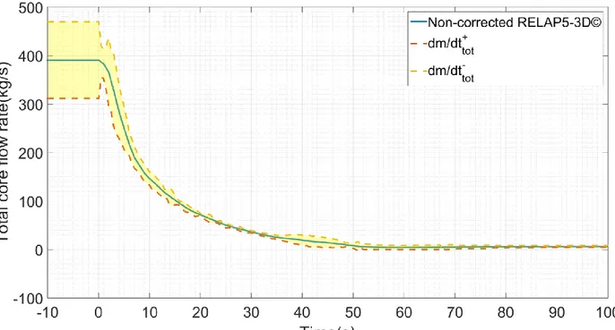
For the above reasons, it became necessary to make a sensitivity analysis of the problem with respect to the flow rates data, by setting two “worst-cases” bounds to the calculation. In these cases, the entire core flow rate was increased or decreased by a certain percentage correction factor, corresponding to the worst relative error among the two instrumented assemblies XX09 and XX10, in the following way:
{ 𝑚̇𝑖+(𝑡) = 𝑚̇𝑖,𝑅𝐸𝐿𝐴𝑃5−3𝐷©(𝑡) ∙ 𝐶𝐹(𝑡) 𝑚̇𝑖−(𝑡) = 𝑚̇ 𝑖,𝑅𝐸𝐿𝐴𝑃5−3𝐷©(𝑡) ∙ 𝐶𝐹(𝑡) 𝐶𝐹(𝑡) = 𝑚𝑎𝑥 {1 −|𝑚̇𝑋𝑋09,𝑒𝑥𝑝(𝑡) − 𝑚̇,𝑖𝑛𝑠𝑡𝑟𝑅𝐸𝐿𝐴𝑃5−3𝐷©(𝑡)| 𝑚̇𝑋𝑋09,𝑅𝐸𝐿𝐴𝑃5−3𝐷©(𝑡) } (13)
The hypothesis lying at the base of the sensitivity analysis assessed with the above flow rates sets is that no information is known on the accuracy of the distribution of the total flow rate among the different HAs, and therefore a computed misdistribution of the flow rate of the same entity could have happened in the HAs around the instrumented ones as well. Total mass flow rates used as maximum and minimum bounds for the sensitivity study are shown along with the RELAP5-3D© non-corrected one in Figure 26.
Figure 26. Comparison between the post-blind RELAP5-3D© flow rates and the corrected flow rates for sensitivity analysis 𝒎̇𝒊+ and 𝒎̇𝒊−.
The expected output, should the hypothesis prove correct and the misdistribution of flow rates is similar to the instrumented assembly in the neighboring zone, is to gain an improvement in XX10 behavior. The XX09 temperature profile, already well described using RELAP5-3D© BCs, may instead be worsened.
These are the different sets of BCs used in the following sections:
BC-1, corresponds to the blind phase RELAP5-3D© flow rates, rescaled by the error of the RELAP5-3D© pump#2 total flow rate with respect to the experimental one. When this set was used, experimental data were already available, but RELAP5-3D© calculations had not been re-performed yet (Nov 2014). For a more detailed description of these flow rates data and their detailed results when used with FRENETIC before the BIB model implementation please refer to [12].
BC-2, corresponds to the post-blind phase RELAP5-3D© flow rates without any correction.
BC-3, refers to the above mentioned 𝑚̇𝑖𝑛+, where the post-blind phase RELAP5-3D©
flow rates have been increased by a correction factor that takes into account the error of RELAP5-3D© with respect to experiments on instrumented assemblies.
BC-4, refers to the above mentioned 𝑚̇𝑖𝑛−, where the post-blind phase RELAP5-3D©
flow rates have been reduced by a correction factor that takes into account the error of RELAP5-3D© with respect to experiments on instrumented assemblies.
The experimental flow rates are superimposed in each of the cases in XX09 and XX10 HAs. The above flow rates boundary conditions sets are summarized in Table 1.
Table 1. Summary of the flow rates data sets used for the various FRENETIC simulations.
Name Flow rates description
BC-1 dm/dtin from RELAP5-3D© (Blind phase) rescaled according to the ratio
between experimental and RELAP5-3D© for pump#2 BC-2 dm/dtin from RELAP5-3D© (Post-Blind phase)
BC-3 dm/dtin from RELAP5-3D© (Post-Blind phase) increased by the maximum
relative difference between the experimental and RELAP5-3D© data in instrumented HAs
BC-4 dm/dtin from RELAP5-3D© (Post-Blind phase) decreased by the maximum
relative difference between the experimental and RELAP5-3D© data in instrumented HAs
3.2.2 Box-in-the-box results
In the following section, steady state and transient results are reported separately. In the last subsection a heat transfer interpretation of the model effectiveness is presented.
Results refer to XX09 and XX10 instrumented assemblies of the EBR-II reactor that were present in the core at the time of the test, the first being a fuelled assembly and the second being a dummy (stainless steel pins) one for which experimental data were made available within the framework of an international IAEA Benchmark.
3.2.2.1 Steady state
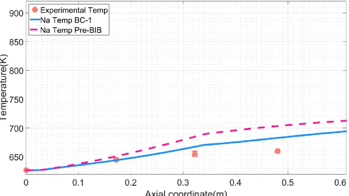
The steady state (t = 0 s, before the start of the transient) distributions of temperature along the axial coordinate of the instrumented assemblies XX09 and XX10 are presented in Figure 27 and Figure 28.
Figure 28. Steady state axial temperature distribution in instrumented assembly XX10: comparison between old (pre-BIB) model and new BIB model with the same set of flow rates boundary conditions (BC-1).
The new BIB model brought a slight improvement in the steady state axial distribution of temperatures in both the assemblies. It must be noted that the underestimation at the mid-core height (MTC = 0.322 m) is due to the assumption, suggested by Argonne, that the input power should be uniformly distributed over the core active length.
XX10 is more affected than XX09 by the presence of the thimble. This goes into the expected direction considering the following two elements:
With respect to the old model, a higher flow rate is considered, the one flowing inside the thimbles of XX10 and XX09. A portion of the power generated in the surroundings of XX10 (which is “colder” than its surrounding HAs) and of XX09 (which is somewhat at an average temperature with respect to its surrounding HAs) is extracted from the core by the thimble flow rate, therefore reducing the temperature of both of them. The steady state linear power distribution in the surroundings of instrumented assemblies is shown in Figure 29.
Figure 29. Steady state linear power (kW/m) distribution in the surroundings of instrumented assemblies XX09 and XX10.
Referring to Figure 18, the relative weight of the thimble flow rate in XX10 assembly is higher than in XX09. For this reason the improvement of XX10 behavior is more evident than that of XX09, which anyhow falls in a very wide range of experimental values coming from the thermocouples.
Even if the situation has got better, the simulated XX10 still reaches a too high temperature both in the active region of the core (where it should be below the experimental one due to the above stated hypothesis of the power uniformly distributed) and in the upper, non-heated, part of the domain.
Once the experimental data were available from ANL, after the blind phase of the IAEA-CRP, the boundary conditions were recomputed by ENEA with RELAP5-3D, and a new simulation on FRENETIC was set, with the so-called BC-2 flow rates. Contrarily to BC-1, where data were rescaled to take into account the relative difference between the experimental and RELAP5-3D© pump behavior (experimental data were already available but new BC had not yet been sent by ENEA), in BC-2 rough data from RELAP5-3D© have been adopted without any rescaling. These data were tuned on experimental results and therefore are supposed to be more accurate than BC-1 data. BC-2 steady state temperature axial distributions are shown in Figure 30 and Figure 31 for instrumented assemblies XX09 and XX10.
Figure 30. Steady state axial temperature distribution in instrumented assembly XX09: comparison between BC-1 and BC-2 sets of flow rates boundary conditions.
Figure 31. Steady state axial temperature distribution in instrumented assembly XX10: comparison between BC-1 and BC-2 sets of flow rates boundary conditions.
No improvement is actually reached at steady state with the new set of flow rates.
The error made on XX10 with both data sets BC-1 and BC-2 may still be related to an overestimation of heat transferred to the dummy instrumented assembly from its neighboring ones, that are hotter as shown in Figure 29. Providing FRENETIC with BC-2 and comparing the computed results to those of RELAP5-3D© (post-blind phase) it can be noticed that those
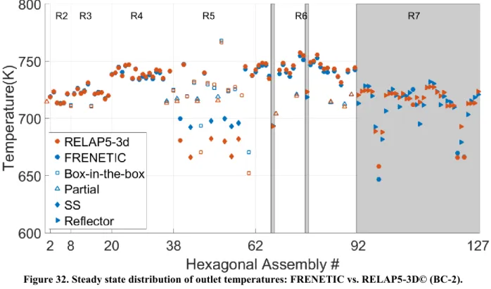
assemblies that the worst represented HAs are actually the stainless steel, dummy ones. This situation is summarized by Figure 32 and Figure 33, where FRENETIC results using BC-2 are compared with RELAP5-3D© steady temperatures at the outlet of the core (obviously with the same flow rates).
analysis has been carried out. Two new BC sets (BC-3 and BC-4) were conceived, that would take into account of the worst error of RELAP5-3D© with respect to known experimental data in both direction (increasing and decreasing the total flow rate). The detailed description of these new sets is provided in Table 1. Results using 3 are compared to the ones obtained with BC-2 in Figure 34 and Figure 35.
Figure 34. Steady state axial temperature distribution in XX09: comparison between BC-2 and BC-3 sets of flow rates conditions.
Figure 35. Steady state axial temperature distribution in XX10: comparison between BC-2 and BC-3 sets of flow rates conditions.
The ~20% increase in the flow rates that has been applied to the BC-2 set to obtain BC-3, brought almost no effect to the steady state axial temperature distribution of XX09 while it showed a non-negligible improvement in XX10 behavior. Since the RELAP5-3D© overestimated XX10 flow rate, if the overestimation is due to a misdistribution of flow rates in that region of the core (i.e. due to inlet orifices or the underestimation of other pressure losses) this could mean that the neighboring subassemblies are less cooled than they should, if the total flow rate is kept constant. If this is verified, increasing the neighboring flow rates keeping the XX10 flow rate constant and equal to the experimental one (as did by BC-3) should go in the right direction.
BC-4 results are not reported since the flow rate reduction obviously worsened the temperature profiles, both in steady state and during the transient. This is in line with the above mentioned phenomenological hypothesis.
3.2.2.2 Transient
In this section the transient results will be shown in the same succession as in the steady state chapter. All the figures will show the temperature evolution at a specific axial location, referred as TTC (Top-of-Core, z = 0.322 m). Flow rates data sets are identified by plots’ legends, Figure 36 and Figure 37 show the differences coming from the introduction of the BIB model using BC-1. As already stated, the flow rates used for the pre-BIB simulation are equal to BC-1 except for neglecting thimble flow rates.
Figure 36. Temperature evolution at Top-of-Core (TTC, z = 0.322 m) height in XX09: comparison between pre-BIB model and new BIB model with BC-1 flow rates boundary conditions.
Figure 37. Temperature evolution at Top-of-Core (TTC, z = 0.322 m) height in XX10: comparison between pre-BIB model and new BIB model with BC-1 flow rates boundary conditions.
Contrarily to steady state where some improvements were obtained by the implementation of the new BIB model, the transient is practically not affected by the sodium flowing inside the thimble of the instrumented assembly.
The transient, as well as the steady state, has been recomputed after receiving the new data (BC-2) from ENEA, improved thanks to the experimental data made available by ANL. BC-2 results are compared to BC-1 in Figure 38 and Figure 39.
Figure 38. Temperature evolution at Top-of-Core (TTC, z = 0.322 m) height in XX09: comparison between BC-2 and BC-1 flow rates.
Figure 39. Temperature evolution at Top-of-Core (TTC, z = 0.322 m) height in XX10: comparison between BC-2 and BC-1 flow rates.
With the post-blind phase flow rates (BC-2), the instrumented assembly XX09 (which is the fuelled one) is very well represented by FRENETIC: the experimental temperature peak is closely gotten by the computed curve, and in general the curves always stay very close, even if the computed one is a little out-of-phase in hitting the peak and in the descendant part.
XX10 situation is instead worsened, making evident the huge sensitivity of results to flow rates boundary conditions. This is in line with what found beforehand in Section 3.2.1, where it was shown that the BC-2 flow rates computed by RELAP5-3D© made a significant error with respect to experimental ones in particular in the first peak-phase of the transient.
This was at the base of the already described sensitivity study made with BC-3 and BC-4 flow rates (Table 1). The results are shown in Figure 40 and Figure 41.
Figure 40. Temperature evolution at Top-of-Core (TTC, z = 0.322 m) height in XX09: comparison between BC-3 and BC-2 flow rates.
Figure 41. Temperature evolution at Top-of-Core (TTC, z = 0.322 m) height in XX10: comparison between BC-3 and BC-2 flow rates.
As expected by the phenomenological discussion on how they were derived, BC-3 flow rates describe XX10 HA very closely. The correction factor applied to BC-2 to obtain BC-3 and BC-4 was, in fact, derived by the maximum experimental error among the ones on XX10 and XX09, which indeed was the one on the “cold” dummy assembly. For the same reasons, since XX09 flow rates were already close enough to the experimental values computed by RELAP5-3D© and since the correction was applied to all the assemblies of the core, XX09 appears too cold in
the BC-3 simulation due to the increase of the flow rates in its neighboring HAs. The experimental values are anyhow almost always bracketed or captured by BC-2 and BC-3 curves. BC-4 is not reported in the above plots since the results showed an overestimation of the temperature evolution in both the instrumented assemblies. This goes in the expected direction: if the hypothesis and assumptions made in Section 3.2.1 on the nature of the error made by RELAP5-3D© with respect to experimental flow rates proves right, decreasing the flow rate of the assemblies in the surroundings of XX09 and XX10 especially takes the opposite effect in “correcting” the error.
From the above results, it is evident that the quality of the results strongly depends on the flow rates boundary conditions and that the FRENETIC code is able to predict and bracket the evolution of the experimental curves within the uncertainties range of the input.
The lack of difference in the SHRT-17 behaviour simulated with the new BIB model compared to the previous model is due of its great temperature uniformity after the SCRAM has taken place. This effect is due to the very low power driver after the protection system has intervened. However, this is not verified during those transients in which the power does not decrease, for example the SHRT-45R where the reactor is not scrammed. In that situation the difference among the linear power deposited in different channels would lead to a stronger temperature difference among neighboring assemblies and therefore the above mentioned model will still be valid and the thimble would have a non-negligible impact on the solution.
Since in LMFBR full power transients are the most feared and plausible transients due to the positive coolant temperature feedbacks and displacement feedbacks, the BIB model is not a useless feature but an important addition. Reactivity insertion accidents, in fact, usually feature very localized power bursts, that enhance inhomogeneity and for which such a BIB model would better describe the heat transfer phenomena involved.
3.2.3 Radial pin model results
The BC-2 data set has been applied to the simulation with the new pin radial model. The first check that has been made was to verify that, at steady state, the numerical solution behaved as the analytical one considering the geometry of the pin as a full cylinder (Section 3.1.2).
The model has been applied to the steady state situation in this reduced configuration and, after that, data were collected at a specified axial location (z = 0.16 m, which is approximately one half of the heated zone): the temperature of the coolant and the convective heat transfer coefficient computed by FRENETIC have been used as input parameters for the analytical solution evaluation.
Starting from the differential heat conduction equation in cylindrical geometry, at steady state 1 𝑟 𝑑 𝑑𝑟(𝑘𝑟 𝑑𝑇 𝑑𝑟) = −𝑞𝑣 (14)
where 𝑟 is the radial coordinate and 𝑞𝑣 is the volumetric heat generation in the pin. Then,
considering a constant heat conductivity of the pin, we get 𝑞𝑣
𝜖 =𝑛𝑜𝑟𝑚 (Δ𝑇𝑚𝑎𝑥−𝑚𝑖𝑛,𝑎𝑛(𝑟𝑖) − Δ𝑇𝑚𝑎𝑥−𝑚𝑖𝑛,𝑐𝑜𝑚𝑝(𝑟𝑖)) 𝑛𝑜𝑟𝑚(Δ𝑇𝑚𝑎𝑥−𝑚𝑖𝑛,𝑎𝑛(𝑟𝑖))
(16) Computed results against analytical full cylinder solution are shown in Figure 42.
Figure 42. XX10 steady state distribution at a height z = 0.16 m with new radial model vs. full cylinder analytical solution and error with respect to analytical solution.
As it can be noticed, the computed curve is perfectly bracketed between the two analytical ones (max k and min k). The error on the analytical solution (max k) reduces rapidly when the number of nodes of the pin radial discretization increases, as expected.
At steady state, the old model performed well because the parabolic profile represents actually the analytical solution of the cylindrical problem. The difference brought by the model lays in transient temperature distributions inside the pin, when the driver is removed and the profile loses its parabolic shape due to the thermal inertia term of the transient equation and the profile tends to flatten (Figure 43).
At time t = 0 s (steady state), the two profiles are overlapping. This is what is expected, since the parabolic assumption is true when the transient term of the conduction equation is off. At time t = 50 s, being the temperature increasing due to mass flow reduction, the heat has to diffuse through the pin again after the initial redistribution due to the scram. This accumulation of heat in the radial direction was neglected with the old model, and the pin increased its temperature as a whole, therefore the rate of increase was faster (Figure 43).
Figure 43. Pin radial temperature distributions at different times w/ and w/o the new FEM radial model (left t = 0 s and right t = 50 s).
The opposite happens after the peak is reached: the temperature starts to decrease (Figure 44) earlier in the simplified (old) model than in the FEM model (the temperature is lower). The difference in heat diffusion between the two models causes the surface temperatures of the pin to differ in the two models of about 5 K at t = 100 s. As time goes by (t = 150 s) and temperature keeps decreasing, the distance between the two curves is reduced: this is due to the fact that a new equilibrium situation is being approached. When this will be reached, at the end of the transient, the two curves would eventually overlap again for the already mentioned reasons.
Figure 44. Pin radial temperature distributions at different times w/ and w/o the new FEM radial model (left t = 100 s and right t = 150 s).
The steady state axial distribution of temperatures and the temperature evolution at Top-of-Core height (z = 0.322 m) are reported and compared against the experimental data with and without the new pin radial model implementation in Figure 45, Figure 46, Figure 47 and Figure 48. As expected, the two solutions almost coincide at steady state: it may be recalled, that this is because the simplified (old) model accounted for a parabolic temperature distribution inside the pin, which is actually the steady state solution of the cylindrical problem. The small differences (~1 K) in the two curves are due to the fact that, in this model, the axial conduction along the axial direction of the pin is neglected.
The transient shows a difference of 10-15 K with respect to the previous model: this is due to the weight of heat diffusion through the fuel pin, which was absent before. The slope of the increase in coolant temperature is a little less steep, since heat needs more time to diffuse inside the solid. Since the geometrical diffusion of heat is still ongoing when the peak of temperature is hit and the curve of temperature changes its sign, the maximum temperature is lower than that computed with the previous simplified model. The descendant part of the curve is, again, less steep for the same above reasons, up to the point that the new solution eventually gets over the old one obtained through the simplified model, because a new steady state solution (and therefore represented by a parabolic distribution) is reached.
The relatively small effect obtained by the implementation of the new model is again due to the low power deposition inside fuel pins which is only due to the decay heat. For un-scrammed transients, where the power deposited in the fuel pins during the loss-of-flow is comparable with that of the reactor at full power (such as SHRT-45R), the difference between the two models will be higher.
The solution, no matter how small is the improvement obtained in the application to the SHRT-17 transient, goes in the expected direction since it damps the height of the temperature peak,
Figure 45. XX10 steady state temperature axial radial distribution: comparison w/ and w/o new radial model.
Figure 46. XX10 temperature evolution at Top-of-Core (z = 0.322 m): comparison w/ and w/o new radial model.
Figure 47. XX09 steady state temperature axial radial distribution: comparison w/ and w/o new radial model.
Figure 48. XX09 temperature evolution at Top-of-Core (z = 0.322 m): comparison w/ and w/o new radial model.
3.3 Conclusions
The capabilities of the thermal-hydraulic (TH) module of the FRENETIC code have been improved thanks to the addition of new features, such as the “Box-in-the-box” (BIB) and the Pin radial model, which better describe the heat transfer phenomena in the core.
The BIB model brought some improvements to the steady state condition of SHRT-17, while the contribution to the transient evolution was almost negligible. This has been explained with the fact the SHRT-17 is a “scrammed” transient: the absence of the driver leads to a temperature redistribution inside the core that brings neighboring assemblies to be almost in equilibrium during the transient phases, therefore making the presence of the flow in the thimble not a relevant parameter for the analysis. Anyhow the BIB model may be an improvement for those full power transients in which neighboring assemblies will set on different temperature fields depending on the entity of the power deposited.
The radial model, conceived to align the FRENETIC code with current experience and tradition in affirmed fission codes, was shown to have a little impact on foreseeing the coolant temperature due to the fact that the conservation of energy was already achieved in the previous simplified model, but positively affects the quality of the computed average and maximum fuel temperature. The latter is a fundamental parameter to assess the gravity of a nuclear accident and therefore needs accurate prediction by codes.
4 Development of the neutronic module
4.1 Introduction
The neutronic module of the FRENETIC code employs a coarse mesh nodal method to solve the multigroup neutron diffusion equations both for direct and adjoint problems, as well as direct, quasi-static and point kinetics solvers for dynamics problems. In this report, the development and the implementation of additional physics models in the code is documented. The first of which is a model for the decay heat, allowing to account for the time-delay associated with variations of the fission power. Particular attention is given to the development and the implementation of a method of solution for the relevant equations in order to to be able to use the decay heat model together with a quasi-static solver.
4.2 Decay heat model and methods of solution
Accounting for the phenomenon of the decay heat, the system of equations which describe the spatial-temporal evolution of the instantaneous fission power density and the concentration of decay heat precursors may be written as
(17)
where is the concentration of decay heat precursors in decay heat family i, is the decay constant of decay heat family i, is the fraction of the energy produced by fission that appears as decay heat in the decay heat family i such that and is the total number of decay heat precursors families. The total fission power density is defined as
![Figure 8. SHRT-17 core loading pattern for the first eight rings [13].](https://thumb-eu.123doks.com/thumbv2/123dokorg/5609311.68083/12.892.261.663.408.901/figure-shrt-core-loading-pattern-rings.webp)
![Figure 12. SHRT-45R core loading pattern for the first eight rings [13].](https://thumb-eu.123doks.com/thumbv2/123dokorg/5609311.68083/16.892.250.660.108.652/figure-shrt-r-core-loading-pattern-rings.webp)
![Figure 14. SHRT-45R example of experimental data on instrumented assemblies. TTC10 and TTC31 are thermocouple locations in the two assemblies [18]](https://thumb-eu.123doks.com/thumbv2/123dokorg/5609311.68083/17.892.110.798.576.967/figure-example-experimental-instrumented-assemblies-thermocouple-locations-assemblies.webp)
![Figure 15. SHRT-45R time evolution of the EBR-II reactor power [18].](https://thumb-eu.123doks.com/thumbv2/123dokorg/5609311.68083/18.892.110.803.128.525/figure-shrt-time-evolution-ebr-ii-reactor-power.webp)