Numerical simulations of the effects of residual stresses in adhesively bonded composite specimen

A

LMA

M

ATER

S

TUDIORUM

U

NIVERSITÀ DI

B

OLOGNA

________________________________________________

Scuola di Ingegneria e Architettura

-Sede di Forlì-

N

UMERICAL

S

IMULATIONS OF THE EFFECTS

OF

R

ESIDUAL

S

TRESSES IN

A

DHESIVELY

B

ONDED

C

OMPOSITE

S

PECIMEN

Master's Degree in Aerospace Engineering

Author:

Paolo Grasso

Supervisor:

Prof. Enrico Troiani

Academic Year 2014/2015

III Ses

A

BSTRACT

In this work the problem of performing a numerical simulation of quasi-static

crack propagation within an adhesive layer of a bonded joint under Mode I

loading affected by stress field changes due to thermal-chemical shrinkage induced by cure process is addressed. Secondly, a parametric study on fracture

critical energy, cohesive strength and Young's modulus is performed. Finally, a

particular case of adhesive layer stiffening is simulated in order to verify qualitatively the major effect.

KEYWORDS: numerical simulation, FEM, residual stress, adhesive, bonded joint,

A

CKNOWLEDGEMENT

This final work is the emblem of many years of study and sacrifice. It was a very long, challenging and formative experience. Obviously sometimes things went tricky and particularly stressing but I had always the help of my family. So, even if it seems not directly correlated with this particular work, I have anywhere to thank my parents to made me possible to attend this course and to pursuit my desire to become an aerospace engineer. When I was seven years old, my dream was to become a crazy scientist, therefore I'm very satisfied because I'm finally quite close.

I sincerely thank my supervisor professor Enrico Troiani for his intellectual and personal support. He is not only an impressive engineer but his attitude is very positive. I've already had the opportunity to work with him for my previous final work of bachelor's degree, so what made me chose to keep on having experiences with prof. Troiani was a very effective combination of his talents.

C

ONTENTS

LIST OF FIGURES AND TABLES ... 9

INTRODUCTION... 11

1 RESIDUAL STRESSES IN ... 13

BONDED STRUCTURES ... 13

2 EXPERIMENTAL DATA SOURCES ... 17

2.1THE SPECIMEN'S GEOMETRY ... 17

2.2 ESTIMATION OF FRACTURE ENERGY ... 18

2.3CALIBRATION CURVE DATA ... 21

3 FINITE ELEMENT MODEL DEFINITION ... 23

3.1COHESIVE ZONE MODEL ... 23

3.2MATERIAL PROPERTIES ... 26

3.3ELEMENT TYPES AND MESH GEOMETRY ... 27

3.4THERMAL STEP ... 29

3.5FRACTURE STEP ... 31

4 RESULTS ... 35

4.1PARAMETRIC STUDY ... 35

4.2RESIDUAL STRESSES EFFECT ... 39

4.3REINFORCEMENT EFFECT ... 41

CONCLUSIONS ... 43

APPENDIX A ... 45

APPENDIX B ... 47

L

IST OF FIGURES AND TABLES

fig.1.1: Coefficient of T expansion vs. degree of conversion for and Epoxy adhesive...14

fig.1.2: Chemical shrinkage vs. degree of conversion of an Epoxy adhesive...15

fig.2.1: Dimensions of DCB specimens (Courtesy by John-Alan Pascoe, TU Delft)...18

fig.2.2: CT specimen used to measure fracture toughness...19

fig.2.3: Load-displacement calibration curve of specimen...22

fig.3.1: Traction Separation Laws...24

tab.3.2: Main material properties...26

fig.3.3: View of 2D mesh...27

fig.3.4: View of elementary module of 3D mesh with factor 3...28

fig.3.5: Shear stress...30

fig.3.6: Normal stresses...30

fig.3.7a: View of constrained specimen in simulation environment...31

fig.3.7b:3D view of cracked specimen (deformation scale factor = 3)...32

fig.3.8: a) ellipsoidal crack front; b) walking plasticization wave...32

fig.3.9: Evolution of σ22 in adhesive layer while cracking...33

fig.4.1: Comparison between different fracture critical energy values...36

fig.4.2: Comparison between different cohesive ultimate strength values...37

fig.4.3: Comparison between different Young's modulus values...38

fig.4.5: Location of stiffened epoxy area...41

fig.4.6: Stiffening effect on static peeling...42

fig.A.1: Degree of conversion vs. time of curing process...45

tab.B.1: Results of calibration curve with thermal-chemical shrinkage effect...47

I

NTRODUCTION

The outstanding advantages of composite materials and bonded joints suggest a far more extensive use of composite bonded load-bearing structures instead of the traditional fastened metallic ones.

The main obstacle to the usage of composite bonded structures are the current limiting certification standards. These are often very restrictive mainly due to a hazy knowledge of fatigue phenomenon in composites or sometimes almost absent experimentations. That makes in some cases prohibitive their application, preferring a more reliable, but less efficient, fastened classical solution. Fortunately, the growing knowhow, thanks to experimental and theoretical research, is making possible a more diffused sense of confidence in these technologies. As far as this prevision of technology evolution is considered, the purpose of my work is to explore the way to make a reliable simulation of an adhesive bonded joint quasi-static crack propagation and to face the problems that come up with the considered approach.

I implement also the effect of thermal and chemical shrinkage of the adhesive layer, that would compromise the effectiveness of the joint due to the generation of a thermal-mechanical residual stress field.

In second place, I perform a simulation of a specimen with a reinforcement of a region of the adhesive layer. It consists in locating a higher stiffness adhesive in proximity of the critical point, where the crack propagation becomes unstable. That happens due to unbalance between the external work and the energy absorbed by the material. The purpose of stiffening is delaying this instability, providing a larger load margin through a small and efficient change of local material properties.

The present thesis work is organized as follows:

 Chapter 1 covers the theoretical and experience background related to residual stresses generated during the bonding process. Both thermal and chemical shrinkage and over-cure are considered.

 Chapter 2 describes the reference source of experimental data that will be considered in the comparison with numerical simulation results. It is accompanied by some essential theory explanations.

 Chapter 3 explains extensively how I implemented the finite element model in order to simulate adequately the crack propagation throughout an adhesive bonded joint. I used Abaqus v.6 software.

 In Chapter 4 the main results of simulations are discussed extrapolating some considerations about specimen fracture behavior as function of many crucial parameters.

1 R

ESIDUAL

S

TRESSES IN

B

ONDED

S

TRUCTURES

I think that it is of primary importance to understand the physics behind the generation of residual stresses in the bonding layer and in the interface between adhesive and adherend. That is a relevant problem that should be addressed: the cure process of the bonding layer causes material shrinkage that affect the actual distribution of stresses, anticipating or postponing the plasticization and failure when the joint is loaded. It is for this reason that I spent a relevant part of my Thesis Preparation research to study the peculiar properties of adhesives and the manufacturing and behavior of adhesively bonded joints.

The formation of residual stresses is related to both the discontinuities and through-cure variation of coefficient of thermal expansion and the chemical shrinkage caused by polymerization of the adhesive.

In the first place, the discrepancy of coefficient of thermal expansion between different materials involved in the bonding causes the region around the contact surface to be very stressed. Some adhesives are cured in autoclave at high temperature and pressure (for instance 120°C at 6 atm) and that is a very different environment compared with the usual operative one of 21°C at 1 atm.

In the second place, the adhesive material changes its own properties during the cure process due to the conversion from liquid state to solid form (fig.1.1). That makes the coefficient of thermal expansion to decrease gradually approximately linearly until it is fully cured (*).

(*)

The adhesive is usually intended fully cured when the degree of conversion reaches 0.96 (for more detail see apx.A)

For simulation purposes a constant mean value between 0.65, gelation critical

point, and 1, completely cured, could be used. For instance, as far as the epoxy

adhesive of this report is considered, the chosen mean value is 70x10-6 °C-1 (ref.2).

figure 1.1: Coefficient of T expansion vs. degree of conversion for and Epoxy adhesive

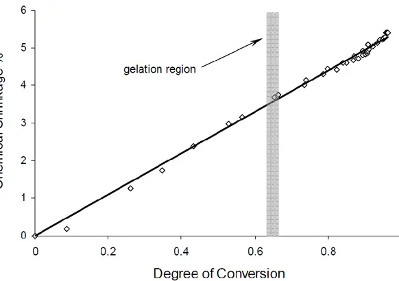
Last but not least, the chemical shrinkage of the adhesive due to polymerization must be considered. The clay starts to warp behind the overlap surfaces of the adherends due to an increase of its own density caused by changes in its chemical structure. A mean value of chemical shrinkage of structural epoxy adhesives is about 6% of volume, that is considerable (fig.1.2).

This last factor is widely neglected by the majority of adhesive and bonded joints studies because of its difficulty to be modeled and predicted. It is neglected even if its influence could be higher than that one of the other factors.

A significant detail is to consider the fact that the residual stress' causes, here described, start to have effect only approximately around the gelation point, when the adhesive reaches a high degree of conversion and starts to adhere strongly to the substrate. Before this critical point, even if some particles are probably chemically connected to the adherend's overlap surface, the relative motion is not constrained because the polymer throw-thickness chains are not completely formed. The gelation point is not precisely detectable but it is manifest by a sharp increase of the adhesive's viscosity.

figure 1.2: Chemical shrinkage vs. degree of conversion of an Epoxy adhesive

Moreover, in the case of composites adhesively bonded structures, there is another challenging problem related to the jointing process. Since the cure takes place at high temperature and pressure, the polymer matrix of sheets, for instance CFRP, will be over-cured, causing its aging and embrittlement. But more considerably adds new enhanced residual stresses between matrix and fibers, that stresses reasonably the last layer of matrix constituting the overlap region.

In order to reduce residual stresses related to the cure process, two main manufacturing solutions could be to design as integral as possible co-cured structures or to perform a low temperature and highly pressurized cure of the adhesive.

2 E

XPERIMENTAL

D

ATA

S

OURCES

AND FEW

T

HEORY

L

UMPS

In order to have a reference with the reality, I used some experimental results of one my co-worker's, N. Zavatta, final project. Regarding this, I will briefly resume the provenance of experimental database and post-processing values that will be successively compared with and used in my 3D simulations.

The aim of the reference thesis work was to investigate the influence of adhesive thickness on adhesively bonded joints under fatigue loading (for more detail see

ref.1). However, for the purposes of my thesis work, I deal only with quasi-static

crack propagation simulations but taking into account the effect induced by cure residual stress field.

Therefore, I will use these following fundamental data.

2.1

T

HE SPECIMEN

'

S GEOMETRY

The specimens were manufactured observing the ASTM Standard

D5528-01(07) that deal fiber-reinforced composite materials' testing for the

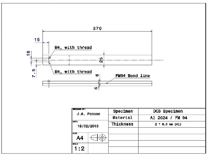
determination of Mode I fracture toughness. The considered specimen is represented in figure 2.1, and the experimental tests were performed on two plates of Aluminum 2024-T3 alloy bonded together by mean of an epoxy adhesive produced by Cytec: FM94 K.03AD FILM 915 (woven nylon in epoxy matrix). More detailed information on manufacture process could be found in reference 1.

Loads were introduced into the specimen by loading blocks screwed to two threaded holes at 15mm far from the left hand side free edge of the top sheet.

figure 2.1: Dimensions of DCB specimens (Courtesy by John-Alan Pascoe, TU Delft)

2.2

ESTIMATION OF FRACTURE ENERGY

In order to explain the meaning of fracture energy, a parameter that I will use with carefulness in my simulations, we have to understand the fracture theoretical model that regards it.

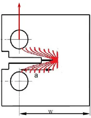
For instance consider a Compact Tension (CT ) specimen (in fig.2.2) that is used for crack toughness measurements. The presence of the crack into the solid modifies considerably the stress field: there's a relieving of the stresses around the crack surface and a highly stress concentrated region plastically deformed about the crack tip.

figure 2.2: CT specimen used to measure fracture toughness

The stress field evolution while the crack is propagating is tightly related to the total structure strain energy flow. For example if crack occurs, some regions, as previously said, result unloaded and that lead to strain energy release. Moreover, a part of the energy is used to break chemical links.

As well as in all physical phenomena an energy balance in required, also the cracking phenomenon is not exempt. The simple Griffith balance formula, appropriate only for brittle materials, could be completed considering all the other possible way of dissipating energy. Follows the modified Griffith equation:

eq.2.1

where is the total strain energy after cracking, is before crack occurs, is the energy release due to crack, is that part required to

break the links, is energy absorbed due to plasticity and finally is the work done by applied forces.

Differentiating this equation by an infinitesimal crack surface area, gathering the dissipative terms ( ), and considering that if

the

strain energy decreases when crack propagates, one can obtain a formula that tells when the unstable crack growth occurs:

eq.2.2

In equation 2.2 one can recognize two parameters. At the left hand side of the equation there is the energy supplied to the crack for its propagation. It is called SERR (Strain Energy Release Rate), usually written as G. At the right hand side, instead, is defined the energy required for the formation of an unit crack area, Gc. Therefore the equation means that the crack growth become unstable when the energy released by cracking is greater than that dissipated. The critical energy release rate could be also written in function of the

fracture toughness (Kc), that is considered as an intrinsic material property

and that can be measured through experiments.

eq.2.3

with E the Young modulus and ν the Poisson’s ratio.

Therefore, the stability criterion could be written in both the ways:

eq.2.4

This parameter is mode dependant: it assume different values for peeling (Mode I), in-plane shear (Mode II) and out-of-plane shear (Mode III). As a rule of thumb, usually the fracture toughness in Mode II and III is two times greater than that of Mode I.

From the results of quasi-static testing (chap.2.3: calibration curve data), it was found the value of critical strain energy per unit area about Gc = 2

N/mm. Not to forget that it refers only to Mode I loading. This value will be

used in the Cohesive Zone Model (CZM ) explained in chapter 4.1.

2.3

C

ALIBRATION CURVE DATA

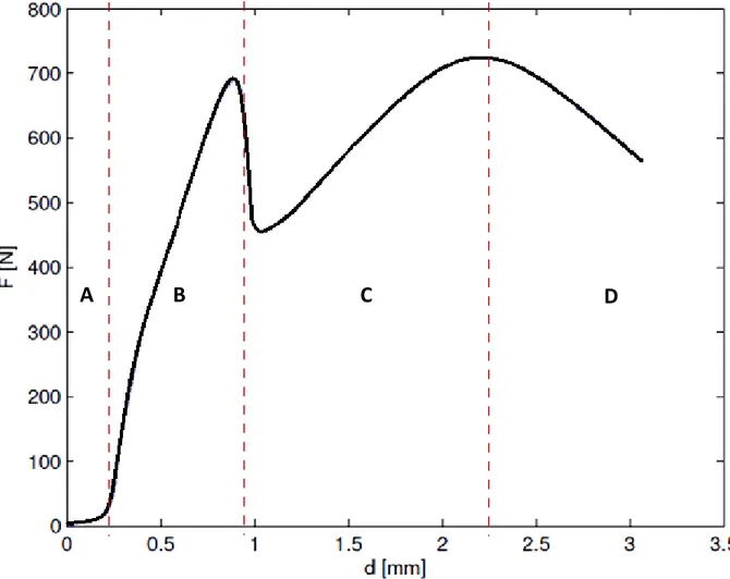
The measurements of calibration curve with quasi-static peeling are considered. Before proceeding with their experiment, they performed a calibration of the tearing machine in order to determine the critical displacement at which the crack growth will be temporally unstable. That was useful for subsequent fatigue tests in order to have the highest possible fatigue crack growth rate, avoiding waste of time. One calibration curve is reported in figure 2.3. It represents the reaction force at the constrained points in function of the displacement imposed by the loading block.

In the fracture process one can recognize four representative regions.

Reg. A - The fist low load bearing lapse is related to the absorption of strain energy by the two free edges of Aluminum sheets that are not bonded.

Reg. B - Then the stiffness value increases because the deformation reaches the joint edge. The epoxy adhesive react to the force applied till it reaches its yield point.

Reg. C - After that it can't bear all the load and it starts to breach. Part of the energy is used to break chemical links for crack propagation, another part is dissipated as heat and the remaining part is plastically absorbed by the following material. It looks like a plasticization wave that propagates

throughout the adhesive layer chased by the crack tip. The reaction force monotonically increases until it reaches another critical point.

Reg. D - It occurs an unstable crack propagation. At higher displacements however, the curve will reach an horizontal asymptote because of geometrical reasons.

figure 2.3: Load-displacement calibration curve of specimen

3 F

INITE

E

LEMENT

M

ODEL

D

EFINITION

The main simulation is intended to reproduce the behavior of specimen used in TU Delft. Firstly, I will describe the Cohesive Zone Model, that is the cohesion model used for simulate the crack propagation within adhesive materials. Secondly, I will define the material properties, finite element types and mesh geometry and I will suggest solutions to some issues regarding this tricky topics. Thirdly, I will explain how to deal with chemical shrinkage and cohesive type elements while simulating the cure step. Finally, I will describe the quasi-static fracture simulation step and the overall history of constraints adopted.

3.1

C

OHESIVE

Z

ONE

M

ODEL

The Cohesive Zone Model (CZM) is primarily intended for simulating bonded interfaces, where the thickness is negligibly small. In this case it could be possible to define the constitutive response of the adhesive material in a more simpler manner. The cohesive behavior can be directly defined in terms of Traction Separation Law (TSL).

The peculiarity of this model are the following:

 it can describe the delamination within composites;

 it permits Mix Mode definition writing fracture energy in function of deformation ratios;

 the final failure is reached through a progressive degradation of the material stiffness, driven by damage accumulation, when the strength becomes zero;

The traction separation law can be uniquely characterized by means of three main parameters. First, the cohesive strength ( ), that is the maximum value of traction bearable by a single cohesive element. Second, the characteristic

length ( ), that is the displacement at which the maximum traction is reached. The third is another parameter that set when complete separation occurs. It could be for instance an ultimate length ( ). For my simulations I used the critical strain energy previously defined (Gc), that is represented by the integral of the TSL curve (fig.3.1).

figure 3.1: Traction Separation Laws

The TSL is applied on all three orthogonal directions n, s and t. The stiffness matrix, that correlates the nominal strain vector, ε, to the stress vector, σ, is obtained in plane strain condition. The stress-strain relation for cohesive layer is the following:

eq.3.1 98%

Where the nominal strain vector's components are:

where T is the cohesive layer thickness, that in my case is about 20μm that is approximately the physical mean dimension of crack opening under fatigue loading.

The stress-strain relation is completed with damage accumulation function

D, that is equal to 0 if the material is considered undamaged, and increases

till 1, that corresponds to final failure of the single cohesive element. In simulations it was computed a linear softening of the material:

eq.3.3

where is obtained from the critical fracture energy, Gc. So the stress-strain relation becomes:

This formulation takes place when the damage initiation criterion is satisfied. There are many criterions available in literature. In my model I implemented the quadratic nominal stress criterion, that seems to be more indicate for a three-dimensional problem.

Moreover, as suggested by some references, for conservative reasons I imposed that the single cohesive element will fail when it reaches the 98% of the fracture energy storable.

3.2

M

ATERIAL

P

ROPERTIES

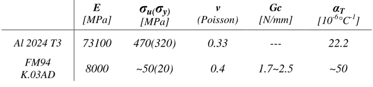
Generally, the values of simulated material can't be the real one, even if we assign some more conservative values to take account of some properties irregularities, such as local difference in chemical composition or local damage, the experimental behavior and the simulated one will never be completely superposed. We consider appreciable a result that has approximately the same parameters trend and order of magnitude. Therefore it is sufficient to assign values of the considered class of materials.

More problems come up considering fracture properties of the material, that are unfortunately dependant on a wide range of parameters. Simulating a reliable fracture scenario is very arduous. For instance, as far as the fracture toughness of the material is considered, it is implicitly assumed that a complex highly correlated in three dimensions problem is reduced to a one-dimensioned parameter, Kc.

More over some correction on the actual material properties have to be made due to finite element model choices. In fact, some values of cohesive material properties must be normalized with respect to the actual thickness of the adhesive layer.

Last but not least, particular attention must be paid to the units. The system of

measure has to be coherent. I used for example time in 's', displacements in

'mm', force in 'N', stresses in 'MPa', critical energy in 'N/mm'.

E [MPa]

σ

σ

α

3.3

E

LEMENT TYPES AND

M

ESH

G

EOMETRY

The fracture phenomenon is a highly discontinuous numerical problem: due to not negligible deformations of the structure and gradual elimination of cohesive elements, it is a bad conditioned problem. Small numerical disturbances could lead to instability and the solver do not reach convergence.

Therefore a first suggestion (other tips will be exposed in chap.3.5) to deal with a bad-conditioned structural problem one should set a regular structured hex mesh without steep changes of shape and dimensions.

However, in order to deal efficiently with meshing the parts, it is suggested to use a fractal partitioning (fig3.3). In fact, this technique allows both to have the maximum required precision in the most discontinuous regions and to reduce considerably the number of nodes in the non-interesting regions.

figure 3.3: View of 2D mesh: a) progressive shrinking of dimension; b) bro- -ken and cancelled cohesive elements; c) still operative cohesive elements.

In the particular case of the treated specimen, the most stressed sections are obviously the cohesive part, the epoxy adhesive part and the interface region between epoxy and adherends. The suggested dimension of a single cohesive element is between 20μm and 250μm, as before explained in chapter 3.1. Then the mesh expands till reaching 4mm in the far field adherends' regions.

Dealing with 3D fractal mesh is geometrically far more complex, because it is generated by interpenetration of two 2D orthogonal meshes that must be coherent. However the classical 3D bricks mesh can not compete in numerical efficiency with this one.

figure 3.4: View of elementary module of 3D mesh with factor 3

A last warning, concerning the mesh, is related to cohesive element type: forgetting to assign the normal direction to the 3D cohesive layer could lead to misunderstandings by the previously defined Traction Separation Law, giving nonsense results or having convergence problems.

3.4

T

HERMAL

S

TEP

Performing a thermal simulation step in order to calculate the residual stress field generated by cure process was challenging for two reasons.

The first issue was to reproduce the volumetric chemical shrinkage of adhesive. Considering the average behavior of epoxy adhesives (refer to

fig.1.2) from gelation point to fully cured, the total strain field could be

written as in the following equation 3.6:

eq.3.6

where is the thermal-chemical strain; is the coefficient of thermal expansion; is the temperature difference; and is the percentage of lengthwise shrinkage. The equation 3.6 is an empirical formula that is only intended to model usefully the two volumetric effects of cure together into one single step. Then one could obtain the modified coefficient of

thermal-chemical expansion, :

eq.3.6a

_eq.3.6b

The second difficulty was related to the assignment of thermal property to the cohesive element. In fact in the case of the software considered, these are not compatible with thermal expansion coefficient. They could be only mechanically loaded, that's the purpose for what they where thought. So, in order to have the fracture step directly after the thermal one, it is necessary to apply a trick. Since the thermal expansion is considered linear, one could set as zero the coefficients of thermal expansion of the cohesive elements the adhesive; and define a relative coefficient of thermal expansion to be applied to the sheets elements.

eq.3.7

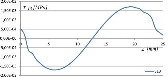
where is the relative coefficient of thermal expansion applied to Aluminum parts; is the modified one and is the actual property. Simulating this model I got the following examples of residual stress shape and order of magnitude. It could be seen quite evidently that, as far as the normal stresses are considered, the main effect of stress redistribution is on the boundaries of the overlap region (z = 0mm and 25mm).

figure 3.5: Shear stress

figure 3.6: Normal stresses * for coordinates refer to fig.3.7a

-2,00E-03 -1,50E-03 -1,00E-03 -5,00E-04 0,00E+00 5,00E-04 1,00E-03 1,50E-03 2,00E-03 0 5 10 15 20 25 S13 -20 -10 0 10 20 30 40 50 60 70 0 5 10 15 20 25 S33 S22

z

z

τ

σ

σ

3.5

F

RACTURE

S

TEP

As far as the actual Fracture Step is considered, one should pay attention to constraint. I respected the actual constraining of the experiment with some reasonable simplifications of force application region. The simulated specimen was arranged as follows.

figure 3.7a: View of constrained specimen in simulation environment

In figure 3.7a the following set-up is shown:

a) mutually bonded edges, they are free to move only along y-axis; b) start of adhesive layer;

c) monotonically increasing displacement application nodes;

d) pinned nodes (U1=U2=U3=0), therefore only rotation about z-axis is allowed;

e) plane of symmetry coincident with the cohesive layer location.

Since it is a bad-conditioned problem, particular attention must be paid to the numerical solver adopted. I used a direct equation solver instead of an iterative one. The solver should account for geometric nonlinearity in this step because the loads on this model result in considerable displacements and

a b

c d e

elimination of some elements.Furthermore, in order to help converging, I set a numerical viscosity of the same order of magnitude of that assigned to the cohesive layer: about 1x10-4. As far as the time step incrementation is considered, it is recommended to perform a discontinuous analysis, that can help to avoid premature cutbacks of the time increment. Finally I choose a minimum time step increment very low, about 10-5, for the same reasons. In

figure 3.7b is shown a screenshot of the cracking specimen while simulating.

figure 3.7b:3D view of cracked specimen (deformation scale factor = 6) And in figure 3.8 the typical ellipsoidal shape of the crack front could be observed and that explain why structural engineers are very concerned about the real crack length that is usually masked by the outer measured crack length.

figure 3.8: a) ellipsoidal crack front; b) walking plasticization wave. a

Finally, in figure 3.9 is evident how the adhesive layer answers to the imposed displacement. At δ =3.5mm the cohesive layer starts to crack, and

that results in unloading the not anymore connected parts.

figure 3.9: Evolution of

σ

cracking; where δ is the opening displacement at load application point and (x-x0) is the distance in longitudinal direction from the crack starting point.

-20 -10 0 10 20 30 40 50 0 5 10 15 20 25 30 35 40 45 0.0 0.2 2.0 4.0 5.0

δ

(x-x

)

σ

4 R

ESULTS

In this chapter many fundamental results are presented. In the first place, I perform a parametric study on the shape of curve of static peeling (chap.4.1). Then I explain the effect of thermal-chemical residual stress field on critical force (chap.4.2). After all, a particular case of adhesive layer reinforcement is considered in order to observe how it affects the behavior of the specimen (chap.4.3).

4.1

P

ARAMETRIC

S

TUDY

Performing the whole simulation, the aim was to reproduce the cracking phenomenon in Mode I. The curve "load vs. displacement" obtained has approximately the same shape and reaches the same critical force value of the experimental calibration curve, but it don't match perfectly. The main probable reason of this mismatch are the following:

1) The actual adhesive properties are not available, particularly the in situ characteristics. I worked on averaged values coherent with the type of material considered.

2) Resins are very dependent on the environment: temperature and humidity change both easily and considerably its own properties.

3) It should be taken into account that possible defects could be present within the real specimen, and these discontinuities interfere surely. Not continuous and not isotropic material properties, and local poor cohesion move away the simulation's results of the ideal specimen from the real one.

4) The inertia of used sensors could also have an effect on the precision, in this case, of measurements. In particular, force measurement could be affected by slight error when the specimen is impulsively unloaded due to cracking. Moreover the actual point of displacement measurement is not precisely defined.

However, I brought to some qualitative results performing a parametric study of the experiment, in order to understand how the main adhesive properties modify the calibration curve shape. I focused on the ultimate

strength,

σ

E

As it is shown in figure 4.1, increasing the fracture toughness of the adhesive results in an enhancement of the maximum peeling load bearable by the specimen. In fact, since the integral Gc is higher, the cohesive element needs to stretch more (greater ultimate length, ) than with a lower value in order to reach maximum damage and that leads also to a higher reaction force due to the fact that the elastic modulus remains the same.

figure 4.1: Comparison between different fracture critical energy values: 1) reference curve at Gc=2N/mm; 2) Gc=1.7N/mm; 3) Gc=2.5N/mm 0 100 200 300 400 500 600 700 800 0 1 2 3 4 5 1 2 3

F [N]

δ [mm]

Instead, if the cohesive strength ( ) is increased the starting slope of the calibration curve become steeper preserving approximately the same critical force (fig.4.2). However, also a changing in shape is observed.

figure 4.2: Comparison between different cohesive ultimate strength values: 1) reference curve at =50MPa; 4) =90MPa; 5) =25MPa

Last but not least, changing the Young's modulus the curve accuses an evident variation of its shape (fig.4.3). I suppose that it is related to the propagation of the plasticization wave throughout the adhesive layer because it is strictly dependant on the strain field.

Even if at first sight the effects of these three parameter seem to be plain, they are highly correlated and they should be analyzed together. However, it is just useful, at first approximation, to recognize these major effects.

0 100 200 300 400 500 600 700 800 0 1 2 3 4 5 1 4 5

F [N]

δ [mm]

figure 4.3: Comparison between different Young's modulus values: 1) reference curve at E=8GPa; 6) E=13GPa; 7) E=3GPa

0 100 200 300 400 500 600 700 800 0 1 2 3 4 5 1 6 7

F [N]

δ [mm]

4.2

R

ESIDUAL

S

TRESSES

E

FFECT

While talking about residual stresses is usually related to something unwanted that disturb the desired behavior of the object analyzed, I found, against my initial thought, that in Mode I loading condition (peeling), the residual stress field of cure is beneficial. In fact the resulting calibration curve reaches an higher force level, within fifty Newton increment (see

fig.4.4).

figure 4.4: A)Reference behavior; B) behavior with RS effect

This peculiar behavior could be explained only if the three-dimensional case is considered. In fact, this effect can not be observed in a two-dimensional simulation. The enlightenment comes from a very simple and basilar relation between normal and transversal strains: the Poisson's effect. A deformation or a stress in one direction will be reproduced in the other two perpendicular directions with opposite sign and revised by the Poisson's coefficient. This effect is particularly evident in gummy materials, but it is also considerable

0 100 200 300 400 500 600 700 800 0 1 2 3 4 5 A B

F [N]

δ [mm]

in resins. For instance, the Poisson's coefficient of the epoxy resin of the specimen is about 0.4 that is quite high. The residual stress field inside the adhesive layer could be briefly described as follows. After cure the adhesive results stretched by the Aluminum adherends in plane directions. Since the resin is not constrained in normal direction, it can freely respect the Poisson's law. It results therefore in a sort of preloading in normal direction of the adhesive. So, this compressive preload should be contrasted enhancing the maximum load bearable by the joint before reaching unstable crack growth. This effect has lower intensity if the adherends and adhesive have approximately the same properties, for example joining CFRP_epoxy with epoxy adhesive. However, the residual stress field is not completely absent because the chemical shrinkage and over-cure problems are still present. So the beneficial effect in mode I is only reduced.

4.3

R

EINFORCEMENT

E

FFECT

The effective crack propagation could also depend on eventual variations of stiffness of the adhesive layer. It could happen if two component clay are not well mixed, or it could be made expressly in order to slow down the crack propagation. Considering this last case, I thought to locate a more rigid epoxy part few millimeters before the place where the crack propagation becomes unstable (approximately 5 mm from the starting crack front till 8 mm).

figure 4.5: Location of stiffened epoxy area

It happens that the stress field between crack tip and stiffened region is considerably modified. In fact, considering the same loading displacement (δ), because of the higher elastic modulus of a not negligible region, the strain are smaller than that of the not-stiffened specimen, so the stress required to get the same critical strain energy release is higher. That is evident in the resulting calibration curve (fig.4.6) where the critical pick force for unstable crack propagation is enhanced of about 80 N assigning to the stiffened part a Young's modulus equal to the Aluminum's one (approximately 73.1 GPa).

region with higher elastic modulus

 unstable  start

figure 4.6: Stiffening effect on static peeling

Usually, it is not necessary to extend the stiffened part more than the critical point, because the real part are obviously designed to work in shear loading conditions. The peel resistance is important to ensure a certain degree of reliability, for instance, in case of secondary-bending loading or eventual fatigue mode I loading. Considering the fatigue loading case, it is quite improbable to load the joint with a maximum displacement higher than the critical one. Therefore, a stiffening as previously defined is enough secure for these cases.

It is not suggested to extend the stiffened part till the starting crack tip, because the high rigidity plastic materials are usually more brittle, and that could be detrimental in fatigue circumstances obtaining a more easy crack propagation. 0 100 200 300 400 500 600 700 800 0 1 2 3 4 5 simple stiffened

F [N]

δ [mm]

C

ONCLUSIONS

The most important result of this research is that the residual stress field induced by thermal-mechanical shrinkage of the cured adhesive layer has beneficial effect

on Mode I loading resistance. In fact, the critical peel loading is considerably

enhanced so the unstable crack propagation is delayed. Performing a parametric study it was found that:

 a greater fracture critical energy (Gc) leads to a higher critical load (Fc);

 increasing the cohesive strength ( ), the major effect is to increase the initial calibration curve slope;

 changing the stiffness of adhesive has the only effect of modifying the curve's shape.

Moreover, if a stiffening part is incorporated into the adhesive just before the critical point, the improvement is far more evident than that of thermal effect. The stiffening gain is about 10% instead of the thermal one of approximately 4%. As far as the intrinsic numerical problems due to bad-conditioning of cracking simulation are considered, one could observe the following advices: to use a fractal 3D mesh enhancing the precision in the most discontinuous regions and relaxing in the far field regions; to use a non linear geometry discontinuous solver; to set a minimum time step increment very low (about 10-5)and to add a bit of numerical viscosity.

Although numerical tools available in commercial FEM software (Abaqus v.6) are useful for a first insight of the simulated problem, they are too restrictive for a deeper analysis. In fact, considering the particular case of fracture, one should produce its own fem program in order to be far more versatile an open minded to new theoretical breakthroughs, as the new energy approach could be considered compared to the classical Linear Elastic Fracture Model (LEFM). However,

instead of writing an entire fem solver, one could make the scrip work in parallel with the FE software, and use the last one as simple automatic calculator of strain and stress fields and to manage the mesh. Moreover, for fatigue simulation it is essential to take this way, inserting the chosen fatigue model in the user defined script, because performing a full fatigue analysis is very time consuming.

A

PPENDIX

A

The degree of conversion represents the fraction of adhesive that is almost completely cured. The relation between the degree of cure reached and cure time is here reported in eq.A.1 and depicted in fig.A.1. The adhesive material is often intended fully cured when it reaches a 0.96 degree of conversion.

eq.A.1

figure A.1: Degree of conversion vs. time of curing process

A

PPENDIX

B

tab.B.1: Results of calibration curve with thermal-chemical shrinkage effect. - none - T-effect t [s] d [mm] F [N] t [s] d [mm] F [N] 0 0 0 0 0 0,00E+00 0,001 0,00045 0,140563 0,001 0,000496 7,15E-02 0,002 0,0009 0,284377 0,002 0,000992 3,01E-01 0,003 0,00135 0,42744 0,0035 0,001736 5,51E-01 0,0045 0,002025 0,641849 0,00575 0,002852 9,15E-01 0,00675 0,003038 0,963442 0,00912 0,004526 1,46E+00 0,010125 0,004556 1,44585 0,01419 0,007038 2,28E+00 0,015188 0,006834 2,16948 0,02178 0,010804 3,50E+00 0,022781 0,010252 3,25505 0,03317 0,016454 5,34E+00 0,034172 0,015377 4,88334 0,05026 0,02493 8,10E+00 0,051258 0,023066 7,32587 0,07589 0,037642 1,22E+01 0,076887 0,034599 10,9893 0,11433 0,056712 1,84E+01 0,11533 0,051899 16,4855 0,172 0,085316 2,77E+01 0,172995 0,077848 24,7293 0,25849 0,128221 4,17E+01 0,259493 0,116772 37,0968 0,38824 0,19258 6,26E+01 0,389239 0,175158 55,6543 0,58286 0,289118 9,41E+01 0,437894 0,197052 62,6114 0,78286 0,388325 1,26E+02 0,510876 0,229894 73,0514 0,98286 0,487532 1,59E+02 0,62035 0,279157 88,7145 1,18286 0,586739 1,90E+02 0,78456 0,353052 112,217 1,38286 0,685946 2,22E+02 0,98456 0,443052 140,644 1,58286 0,785152 2,52E+02 1,18456 0,533052 168,535 1,78286 0,884359 2,82E+02 1,38456 0,623052 196,32 1,98286 0,983565 3,12E+02 1,58456 0,713052 223,558 2,18286 1,082775 3,41E+02 1,78456 0,803052 250,419 2,38286 1,181975 3,70E+02 1,98456 0,893052 277,122 2,58286 1,281185 3,98E+02 2,18456 0,983052 303,185 2,78286 1,380395 4,26E+02 2,38456 1,07305 328,996 2,98286 1,479605 4,54E+02 2,58456 1,16305 354,592 2,99536 1,485805 4,55E+02 2,78456 1,25305 379,59 2,99848 1,487355 4,56E+02 2,98456 1,34305 404,33 3,00317 1,489675 4,57E+02 3,18456 1,43305 428,746 3,0102 1,493165 4,57E+02 3,23456 1,45555 434,701 3,02075 1,498395 4,59E+02 3,28456 1,47805 440,598 3,03657 1,506245 4,61E+02 3,33456 1,50055 446,431 3,0603 1,518015 4,64E+02 3,40956 1,5343 455,123 3,0959 1,535675 4,69E+02 3,52206 1,58493 468,087 3,14929 1,562155 4,76E+02 3,69081 1,66086 486,934 3,22938 1,601885 4,86E+02 3,89081 1,75086 508,271 3,34951 1,661475 5,02E+02

4,09081 1,84086 528,49 3,52972 1,750865 5,24E+02 4,29081 1,93086 546,347 3,72972 1,850065 5,47E+02 4,49081 2,02086 559,833 3,92972 1,949275 5,67E+02 4,69081 2,11086 566,249 4,12972 2,048485 5,84E+02 4,89081 2,20086 570,187 4,32972 2,147685 5,90E+02 5,09081 2,29086 578,425 4,52972 2,246895 5,97E+02 5,29081 2,38086 588,502 4,72972 2,346105 6,05E+02 5,49081 2,47086 599,782 4,92972 2,445315 6,18E+02 5,69081 2,56086 612,895 5,12972 2,544515 6,31E+02 5,89081 2,65086 625,485 5,32972 2,643725 6,45E+02 6,09081 2,74086 638,316 5,52972 2,742935 6,61E+02 6,29081 2,83086 652,205 5,72972 2,842135 6,76E+02 6,49081 2,92086 666,042 5,92972 2,941345 6,90E+02 6,69081 3,01086 679,041 6,12972 3,040555 7,05E+02 6,89081 3,10086 691,709 6,32972 3,139755 7,20E+02 7,09081 3,19086 702,97 6,52972 3,238965 7,30E+02 7,29081 3,28086 702,105 6,72972 3,338175 7,27E+02 7,49081 3,37086 694,384 6,92972 3,437375 7,12E+02 7,69081 3,46086 676,089 7,12972 3,536585 6,92E+02 7,89081 3,55086 656,491 7,32972 3,635795 6,73E+02 8,09081 3,64086 640,245 7,52972 3,735005 6,56E+02 8,29081 3,73086 625,59 7,57972 3,759805 6,45E+02 8,49081 3,82086 613,342 7,65472 3,797005 6,36E+02 8,69081 3,91086 605,267 7,76722 3,852805 6,32E+02 8,89081 4,00086 596,813 7,93597 3,936515 6,24E+02 9,09081 4,09086 588,434 8,13597 4,035725 6,16E+02 9,29081 4,18086 580,372 8,33597 4,134925 6,08E+02 9,49081 4,27086 574,52 8,53597 4,234135 6,01E+02 9,69081 4,36086 568,196 8,73597 4,333345 5,93E+02 9,89081 4,45086 562,668 8,93597 4,432545 5,85E+02 10 4,5 557,678 9,136 4,531755 5,79E+02 9,336 4,630965 5,73E+02 9,536 4,730165 5,65E+02 9,736 4,829375 5,58E+02 9,936 4,928585 5,53E+02 10 4,960345 5,49E+02

tab.B.1: Results of calibration curve with stiffening region. - none - stiffened t [s] d [mm] F [N] t [s] d [mm] F [N] 0,001 0,00045 0,140563 0,001 0,00045 0,140871 0,002 0,0009 0,284377 0,002 0,0009 0,285003 0,003 0,00135 0,42744 0,003 0,00135 0,42838 0,0045 0,002025 0,641849 0,0045 0,002025 0,643258 0,00675 0,003038 0,963442 0,00675 0,003038 0,965558 0,010125 0,004556 1,44585 0,010125 0,004556 1,44903 0,015188 0,006834 2,16948 0,015188 0,006834 2,17424 0,022781 0,010252 3,25505 0,022781 0,010252 3,26219 0,034172 0,015377 4,88334 0,034172 0,015377 4,89404 0,051258 0,023066 7,32587 0,051258 0,023066 7,34192 0,076887 0,034599 10,9893 0,076887 0,034599 11,0134 0,11533 0,051899 16,4855 0,11533 0,051899 16,5216 0,172995 0,077848 24,7293 0,172995 0,077848 24,7835 0,259493 0,116772 37,0968 0,259493 0,116772 37,1782 0,389239 0,175158 55,6543 0,389239 0,175158 55,7763 0,437894 0,197052 62,6114 0,437894 0,197052 62,7486 0,510876 0,229894 73,0514 0,510876 0,229894 73,2115 0,62035 0,279157 88,7145 0,62035 0,279157 88,9091 0,78456 0,353052 112,217 0,78456 0,353052 112,463 0,98456 0,443052 140,644 0,98456 0,443052 140,963 1,18456 0,533052 168,535 1,18456 0,533052 168,925 1,38456 0,623052 196,32 1,38456 0,623052 196,781 1,58456 0,713052 223,558 1,58456 0,713052 224,101 1,78456 0,803052 250,419 1,78456 0,803052 251,042 1,98456 0,893052 277,122 1,98456 0,893052 277,827 2,18456 0,983052 303,185 2,18456 0,983052 303,974 2,38456 1,07305 328,996 2,38456 1,07305 329,868 2,58456 1,16305 354,592 2,58456 1,16305 355,546 2,78456 1,25305 379,59 2,78456 1,25305 380,635 2,98456 1,34305 404,33 2,98456 1,34305 405,468 3,18456 1,43305 428,746 3,18456 1,43305 429,978 3,23456 1,45555 434,701 3,23456 1,45555 435,96 3,28456 1,47805 440,598 3,28456 1,47805 441,889 3,33456 1,50055 446,431 3,33456 1,50055 447,764 3,40956 1,5343 455,123 3,40956 1,5343 456,517 3,52206 1,58493 468,087 3,52206 1,58493 469,59 3,69081 1,66086 486,934 3,69081 1,66086 488,708 3,89081 1,75086 508,271 3,89081 1,75086 510,514 4,09081 1,84086 528,49 4,09081 1,84086 531,651 4,29081 1,93086 546,347 4,29081 1,93086 551,561 4,49081 2,02086 559,833 4,49081 2,02086 569,291 4,69081 2,11086 566,249 4,69081 2,11086 582,78

4,89081 2,20086 570,187 4,89081 2,20086 593,802 5,09081 2,29086 578,425 5,09081 2,29086 604,331 5,29081 2,38086 588,502 5,29081 2,38086 617,818 5,49081 2,47086 599,782 5,49081 2,47086 631,601 5,69081 2,56086 612,895 5,69081 2,56086 645,456 5,89081 2,65086 625,485 5,89081 2,65086 661,84 6,09081 2,74086 638,316 6,09081 2,74086 677,667 6,29081 2,83086 652,205 6,29081 2,83086 693,912 6,49081 2,92086 666,042 6,49081 2,92086 709,933 6,69081 3,01086 679,041 6,69081 3,01086 726,57 6,89081 3,10086 691,709 6,89081 3,10086 742,468 7,09081 3,19086 702,97 7,09081 3,19086 756,471 7,29081 3,28086 702,105 7,29081 3,28086 768,728 7,49081 3,37086 694,384 7,34081 3,30336 770,418 7,69081 3,46086 676,089 7,35956 3,3118 770,653 7,89081 3,55086 656,491 7,38768 3,32446 755,949 8,09081 3,64086 640,245 7,41581 3,33711 714,812 8,29081 3,73086 625,59 7,44393 3,34977 676,132 8,49081 3,82086 613,342 7,48612 3,36876 636,885 8,69081 3,91086 605,267 7,5494 3,39723 617,079 8,89081 4,00086 596,813 7,64433 3,43995 603,277 9,09081 4,09086 588,434 7,78671 3,50402 597,514 9,29081 4,18086 580,372 7,98671 3,59402 594,573 9,49081 4,27086 574,52 8,18671 3,68402 594,369 9,69081 4,36086 568,196 8,38671 3,77402 591,403 9,89081 4,45086 562,668 8,58671 3,86402 590,225 10 4,5 557,678 8,78671 3,95402 585,603 8,98671 4,04402 581,684 9,18671 4,13402 576,349 9,38671 4,22402 571,454 9,58671 4,31402 564,663 9,78671 4,40402 559,697 9,98671 4,49402 552,69 10 4,5 550,377

R

EFERENCES

[1] Nicola Zavatta, "Influence of adhesive thickness on adhesively

bonded joints under fatigue loading", Aerospace Engineering Master

Degree , 2015

[2] Mauro Zarrelli, Alexandros A Skordos and Ivana K Partridge,

"Investigation of cure induced shrinkage in unreinforced epoxy resin" Advanced Materials Dept, Cranfield University, Cranfield,

Bedford, MK430AL, UK

[3] F.S. Jumbo, I.A. Ashcroft1, A.D. Crocombe and M.M Abdel Wahab,

"Thermal Residual Stress Analysis of Epoxy Bimaterial Laminates and Bonded Joints"

[4] W.R. Broughton and G. Hinopoulos, "Evaluation of the Single-Lap

Joint Using Finite Element Analysis"

[5] H. Jiang, “Cohesive Zone Model for Carbon Nanotube Adhesive

Simulation and Fracture/Fatigue Crack Growth”. University of

Akron, 2010.

[6] K. Park and G.H. Paulino, “Cohesive Zone Models: A Critical

Review of Traction-Separation Relationships Across Fracture Surfaces”. In: Applied Mechanics Reviews 64(6), 060802 (2011).

[7] J.A. Pascoe, R.C. Alderliesten, and R. Benedictus. “On the

relationship between disbond growth and the release of strain energy”. In: Engineering Fracture Mechanics 133, 1-13 (2014).

[8] D. Roylance, “Introduction to Fracture Mechanics”. Department of Materials Science and Engineering, MIT, 2001.

[9] Dassault Systèmes, Abaqus Analysis User’s Manual, Version 6.7. url: http://www.egr.msu.edu/software/abaqus/Documentation/docs/ v6.7/books/usb/default.htm?startat=pt06ch26s05alm40.html.

[10] J.W.van Ingen and A. Vlot, "Stress Analysis of Adhesive Bonded

SLJ"

[11] Jean - Pierre Pascault and Roberto J.J. Williams, "chap.1: General

Concepts about Epoxy Polymers"

[12] Michael J. Hoke Abaris "Adhesive Bonding of Composites": lecture notes,Training Inc.

[13] Alberto Sánchez Cebrián "Bonding of Composites Structures": lecture notes