Cold wire thermometry for turbine measurements

(1)

POLITECNICO DI MILANO

Facoltà di Ingegneria Industriale e dell’Informazione

Corso di Laurea in

Ingegneria Aeronautica

COLD WIRE THERMOMETRY

FOR TURBINE MEASUREMENTS

Relatore: Prof. Carlo Osnaghi

Co-relatore: Dr. Sergio Lavagnoli

Tesi di Laurea di:

Guido LATORRE Matr. 799309

(2)

(3)

III

(4)

(5)

V

List of Figures

Figure 1.1 Section view of the Rolls-Royce Trent 1000……….…….1

Figure 2.1 The turbine test rig of Von Karman Institute……….6

Figure 2.2 A schematic representation of CT3………...7

Figure 2.3 Setup for the calibration of cold wire………8

Figure 2.4 Metallic supports………. 9

Figure 2.5 Metallic tool designed in CATIA………10

Figure 3.1 Configurations of thermocouples………..………..12

Figure 3.2 Electric polarity of metals function of temperature…………13

Figure 3.3 Characteristic curve of a thermocouple without reference zone box...13

Figure 3.4 Thermocouple measurement with a reference box…………...14

Figure 3.5 Measurements with a reference zone box-second configuration……….. 14

Figure 3.6 Reference system for thermocouple steady errors…………. 16

Figure 3.7 Julabo 12-b oil-bath……… 19

Figure 3.8 Stabilization of temperature of cold wire……… 20

Figure 3.9 Table with calibration values of thermocouples………. 20

Figure 3.10 Calibration curve of 4R thermocouple……… 21

Figure 3.11 Principle of resistance thermometer……… 22

Figure 3.12 The effect of convection (velocity) on the cut-off frequency ……… 25

Figure 3.13 Particular of a cold wire: the wire is suspended between two stain prongs……….. 26

(8)

VIII

Figure 3.15 Transfer function of the wire-prong system……… 29

Figure 3.16 Cold wires DAO121A, DAO123A………. 30

Figure 3.17 Setup for the static calibration in the oven………. 31

Figure 3.18 Schematic representation of the wiring of a cold wire……… 32

Figure 3.19 Stability of the white box TUCW2……... 33

Figure 3.20 Results of the static calibration in the oven of the two cold wires

DAO121A, DAO123A……… 34

Figure 3.21 Experimental setup for the static calibration of the cold wire in the

jet……… 35

Figure 3.22 The cold wire boxes (Wheatstone bridge)……….. 36

Figure 3.23 Setup for the calibration of the SENSYM (differential pressure

transducer)……….. 37

Figure 3.24 Calibration curve of the SENSYM R4S4………... 38

Figure 3.25 Thermocouple 4R (up) and cold wire (put horizontally)…… 38

Figure 3.26 The heating system for the air pressurized reservoir……….. 39

Figure 3.27 Comparison of head 2A before and after reparation………... 43

Figure 4.1 Filter boxes……….. 46

Figure 4.2 Electronic cards. The filter boxes are supplied by

electronic cards………47

Figure 4.3 The frequency generator is used to produce signal of known shape

and frequency……….. 48

Figure 4.4 GENESIS data acquisition system……….. 49

Figure 4.5 Experimental setup for filter boxes tests………. 51

Figure 4.6 The output of the acquisition obtained with Perception……. 52

Figure 4.7 The acquired sinusoidal signal is affected by noise that has to be

corrected……….. 53

Figure 4.8 The sinusoidal signal crosses the zero several times generating a

(9)

IX

Figure 4.9 An example of cross-correlation………. 55

Figure 4.10 The signal before and after having used the ‘smooth’ function in Matlab………. 56

Figure 4.11 The Fast Fourier Transform of a signal allows to find the frequency content of a signal………... 56

Figure 4.12 High-Pass Gain………58

Figure 4.23 Raw Phase shift……….. 64

Figure 4.25 Example of a cold wire step signal………..68

Figure 4.26 Configuration of a cold wire………... 68

Figure 4.27 Comparison of the computed first order transfer function with the one found by Dénos……… 71

Figure 4.28 Comparison between the computed two order transfer function with the one found by Dénos……….. 74

Figure 4.29 Comparison between the computed five first order transfer function and the one obtained by Dénos………. 77

Figure 5.1 Physical characteristics and calibration coefficients of cold wire DAO123A………... 81

Figure 5.2 Step test with calibration coefficients of the test done at Mach 0 ……… 83

Figure 5.3 Step test with calibration coefficients of the test done at Mach 0.05 ……… 84

Figure 5.4 Step test with calibration coefficients of the test done at Mach 0.05; a shift has been subtracted to the cold wire signal………… 85

Figure 5.5 Step test 1 at Mach 0.05………. 86

Figure 5.6 Step test 1 at Mach 0.1……… 86

Figure 5.9 The setup used to realize the step tests……….88

(10)

X

Figure 5.11 Step test 2 at Mach 0.1……….. 89

Figure 5.12 Step test 2 at Mach 0.2……….. 90

Figure 5.14 Comparison between the cold wire step signal and the theoretical

Heaviside step………. 93

Figure 5.15 Fast Fourier Transform of the cold wire signal (blue and the

Heaviside signal (red)………. 93

Figure 5.16 The ratio of the FFT of the cold wire signal and the FFT of the

Heaviside input signal gives the experimental transfer function………... 94

Figure 5.17 The impulse has been obtained subtracting two consecutively

values of the original signal and dividing this value by the delta time between them……….. 95

Figure 5.18 The resulting transfer function obtained after having redefined the

step impulse………. 96

Figure 5.19 The theoretical true step is the step generated by the movement of

the shield………. 97

Figure 5.20 The signal of the cold wire has been cleaned from spurious peaks,

low-pas filtered and adimensionalized……… 98

Figure 5.21 The experimental transfer functions found with ‘tfest’ with a

different number of poles, tested at Mach number 0.05……. 98

Figure 5.22 The modified transfer function combines the low frequency

behaviour of the experimental transfer function found with ‘tfest’ and the high frequency behaviour typical of the tungsten wire ………. 100

Figure 5.23 The transfer functions found with ‘tfest’ imposing different

number of poles in step tests at Mach number 0.3………….. 101

Figure 5.24 The cold wire signal has been compensated using the inverse of

the transfer function……… 102

Figure 5.25 The transfer function (blue) and its inverse (red) used for the

(11)

XI

Figure 5.26 The probes are inserted in these metallic supports…………. 106

Figure 5.27 The setup used to set the depth and the angle of the probe in the

turbine channel……… 106

Figure 5.28 The RPM during the test in the turbine rig………. 108

Figure 5.29 The pressure sensed by the differential pressure transducers during

the test in the turbine rig………. 109

Figure 5.30 Comparison of the signals of the two heads of cold wire

DAO123A………... 110

Figure 5.31 The transfer function of 3rd order obtained with step tests for

different Mach numbers……….. 112

Figure 5.32 Comparison of the raw signal of the cold wire and the compensated

raw signal of the cold wire……….. 113

Figure 5.33 Compensation with the transfer function obtained at

Mach=0.05………... 114

Mach=0.1……… 114

Mach=0.2………. 115

Mach=0.3………. 115

(12)

(13)

XIII

List of tables

Table 3.1 Electrical and physical properties of couples-wires……...12

Table 3.2 Results of calibration of the thermocouples 4R and Ttube…...22

Table 3.3 Wiring of the cold wire transducers with the Wheatstone bridge

entries……… 33

Table 3.4 Results of the static calibration of cold wire…………..…...….44

Table 4.1 Range of frequencies analysed for the test of the filter boxes 50

Table 4.2 Data to compute the first order transfer function………. 70

Table 4.3 Data to compute the second order transfer function…………. 73

Table 4.4 Percentage of contribution to (1-g)……… 75

Table 4.5 Data used to compute the fifth order transfer function………. 76

Table 5.1 Calibration coefficients of cold wire DAO123A………. 80

Table 5.2 Calibration coefficients of the pressure transducer 12V8……. 81

Table 5.3 Calibration coefficients of the differential pressure probes

(14)

(15)

XV

Nomenclature

Roman Symbols

𝐴_𝑐 convection heat transfer area [m2]

𝐴_𝑅 radiation heat transfer area [m2]

C absolute velocity of fluid [m/s]

𝐶𝑝 heat capacity at constant pressure [J/(kgK)]

𝐶_𝑝 heat capacity of prong [J/(kgK)]

𝐶_𝑤 heat capacity of wire [J/(kgK)]

𝐶_𝜃 tangential component of absolute velocity [m/s]

𝑑_𝑝 diameter of the prong [m]

dP dynamic pressure , Ptot-Ps [Pa]

𝑑_𝑤 diameter of the wire [m]

F view factor [-]

fcut-off cut-off frequency [Hz]

h convective heat transfer coefficient [W/(m2K)]

𝐼₀ current [A]

𝑘_𝑔 conductivity of the gas [W/(mK)]

𝑘𝑝 conductivity of the prong [W/(mK)]

𝑘𝑤 conductivity of the wire [W/(mK)]

𝑙_𝑤 length of the wire [m]

𝑙_𝑝 length of the prong [m]

M Mach number [-]

(16)

XVI

𝑃𝑠 static pressure [Pa]

𝑃_𝑡𝑜𝑡 total pressure [Pa]

Q heat flux [W]

R resistance [Ω]

R radius [m]

𝑆_{𝑤𝑖𝑟𝑒} surface of the wire [m2]

𝑇_ℎ𝑜𝑡 temperature of the gas [K]

𝑇_{𝑗𝑢𝑛𝑐𝑡𝑖𝑜𝑛} temperature of the junction (thermocouple) [K]

𝑇0 total temperature [K]

𝑇𝑟𝑒𝑓 reference temperature [K]

𝑇_𝑤 wall temperature [K]

𝑣_𝑔 velocity of the gas [m/s]

𝑉_𝑤 volume of the wire [m3]

Greek Symbols α 𝑘𝑤⁄𝜌𝑤 𝑐𝑤 [W/m2] α thermal diffusivity [m2/s] 𝛼𝑤 sensitivity to temperature [1/K] 𝜀𝑤𝑎𝑙𝑙 emissivity [-] Λ2 _{4ℎ 𝑘} 𝑤𝑑𝑤 ⁄ [1/m2]

𝜌_𝑝 density of the prong [kg/m3]

𝜌_𝑤 density of the wire [kg/m3]

γ specific heat ratio [-]

σ Stefan-Boltzmann constant [W/(m2_K4_)]

(17)

XVII

ω angular velocity [rad/s]

τ time constant [s]

(18)

(19)

XIX

Abstract

The aim of this work is the characterization of the dynamic behaviour of a cold wire. The probe has been first calibrated in static conditions in two different ways (oven and heated jet); the dynamic calibration has been realized with temperature step tests. In these tests a shield has been used to isolate the cold wire from an air-heated jet of a certain temperature and Mach number: the shield has been removed abruptly with a finite velocity thus exposing the transducer to the jet. In this way it has been realized a ‘step’ of temperature. This experimental test has been compared to the theoretical step and it was possible to get the transfer function describing the dynamic behaviour of the cold wire at low frequencies. The obtained transfer function has been modified adding the contribution of the tungsten wire in order to take into account the high frequencies: the wire behaves like a first order system whose transfer function can be obtained analytically. The compensation has been obtained using the inverse of the transfer function. Finally the cold wire has been tested in a turbine running at 2200 rpm in vacuum-ambient pressure transient conditions in order to see the effects of compensation

Key words:

cold wire, unsteady conditions, transfer function, conduction effects, compensation, turbine.

(20)

(21)

1

Chapter 1 Introduction

1.1 Research and instrumentation for turbine measurements

The aerospace sector has always been one of the leader in the research investigation and the opening of this industry to the global business has subjected it to an extreme rivalry. In particular, the commercial and civil branch of the aerospace industry has been focused on the reduction of fuel consumption, being the first source of cost for airline companies [1]. The main efforts in research have been addressed to the efficiency of engines, in particular the turbine and compressor stages, Fig.1.1. The numerous unknown mechanisms of fluid dynamic occurring inside aero-engines have become an important challenge in the last years and new measurement techniques have been adopted in order to better describe these phenomena. The main problem of internal fluid dynamics is the per se unsteady behaviour of the flow: due to potential and viscous flow effects, the working fluid experiences rapid periodic changes of total and static pressure, Mach number and flow angle which has to be sensed by innovative technologies.

(22)

2

Nowadays, in spite of the efforts done, we do not dispose of enough information about unsteady flows in air-breathing engines: research has been focused on computational and experimental activities. The computational studies have the advantage to forecast rather accurately fluid dynamics models with a relatively low cost. Nevertheless they do not represent reality but they are an useful tool to estimate physical phenomena: the validation of these numerical works comes from the experimental activity. The experimental investigation of aerothermodynamics phenomena requires a thorough study and a long and expensive effort in order to obtain convincing results: the importance of the measurement techniques adopted become fundamental.

The analysis of flow inside an aero-engines has to take into account complicate aspects of mass and heat transfer and the current technology on the measurement investigation offers a wide choice on instrumentations: pressure transducers (variable capacitance, variable resistance, variable inductance, piezoelectric probes), anemometers (how wire, hot film sensors), thermometry (thermocouples, cold wires, infrared thermography) and optical measurements. The transducers adopted in fluid dynamic research have a wide range of applications and, depending on their accuracy and velocity response, variable costs. The analysis of flow in aero-engine conditions is one of the most complicate due to the extreme rapidity of the phenomena: suitable instrumentations with a high frequency response have to be used to achieve a good scientific survey.

The thermometry and related instrumentation play a fundamental role in the turbomachinery. The analysis of temperature inside the engine is an important parameter to register and study in order to preserve the integrity of the engine itself. The turbine is the component of the engine which is subjected to the most extreme conditions: the rotor has to withstand temperatures around 850-1700°C (depending on the stage of the turbine) and a linear rotation speed that can reach 500 m/s. The current recommendations about the expected engine lifetime cycle states that the engines has to work for 6 years (14 hours/day) before overhaul or replacement and it becomes fundamental a map of the temperature and stress of the components.

Furthermore, the temperatures reached in the different stages are strictly related to the power that the flow supplies to the turbine as the Euler’s equation states:

ṁc_p(T_t2− T_t1) = ω(r₂C_2−θ− r₁C_1−θ) (1.1)

This is a power balance where the total temperature variation across the rotor is

(23)

3

distance respect to the axis of the turbine, 𝐶𝑖−𝜃 is the tangential component of the

absolute velocity of the flow).

Another important motivation of accurate thermometry studies inside engines is associated with the possibility to evaluate the real efficiency of the engines and study new methods in order to increase this parameter.

The most suitable instrumentations for turbines measurements are thermocouples and cold wires. The mechanisms to sense temperature variations are different and also the performances change a lot. The thermocouples are robust and simple instruments used to register temperature variations as a result of a difference of voltage between the extremities of two different metallic wires joined together (Seebeck effect). The cold wire is made of tungsten and inserted inside a balanced Wheatstone bridge: the wire is supplied by a low electric current and its resistance changes with temperature variations. The cold wire is extremely accurate and can have a frequency response one order of magnitude bigger respect to the thermocouple. On the other hand, the cold wire is very fragile, expensive and needs an adequate instrumentations.

1.2 Objectives of the work

The original aim of this thesis was to investigate the behaviour of one-and-a-half turbine stage in similarity conditions with aero-engine. Due to the damage of a component of the facility where the turbine should have been tested, it has been decided to address on other aspects.

The study of this work is focused on the static and dynamic characterization of the cold wire and thermocouples. They have been calibrated with different techniques in static conditions (water-bath, oven, heated jet) and it was possible to extrapolate calibration curves relating temperature and voltage. The same instruments have been tested in dynamic conditions realizing step tests of temperature using a “shield” and a heated jet of a known Mach number and temperature. It was possible to analyse the effect of Mach number in the response of the probes.

In order to overcome the physical limits of the cold wire to reproduce fast temperature variations we obtained several transfer functions referred to tests at different Mach numbers. The signal has been compensated using the inverse of the transfer function thus obtaining an acceptable result of the original true step.

(24)

4

These transfer functions have been used to compensate the signal of the cold wire used inside the CT3 facility of the Von Karman Institute in a vacuum-ambient pressure test.

1.3 Thesis Outline

The thesis is composed of five chapters. It is described the work done at Von Karman Institute from October 2014 to March 2015.

Chapter 1 provides a general description of the new challenges in the research of aero engines and it is given an overview on the thermometry instrumentation. A short paragraph is reserved to the description of the experimental work.

Chapter 2 is dedicated to the description of the experimental apparatus used at VKI, starting from the CT3 facility to the instruments and tools used in the ‘Heat and mass exchange laboratories’.

Chapter 3 gives an accurate description of the working principles and of the static calibration of the thermocouples and cold wires. The results are presented at the end of the chapter.

Chapter 4 offers an overview of the problem of signal filtering and signal compensation. It is described how to characterize analogue filters (i.e. find the Bode diagrams) and how a transfer function determines the dynamic behaviour of a transducer.

Chapter 5 reports the experimental activity. It is shown how the step tests have been realized and how it was possible to extrapolate the experimental transfer functions. The second part of the chapter is dedicated to the description of a test in CT3 and the results registered by the cold wire with the related conclusions.

(25)

5

Chapter 2 Experimental apparatus

The Von Karman Institute for fluid dynamics is a renewed research centre specialized in the application of fluid dynamics in several fields, including environmental engineering, aerospace and turbomachinery. It was founded in 1956 with the aim of Theodore Von Karman, physicist and aerospace engineer, to create an institution specialized in training young engineers in the aerodynamics. Today is one of the most important centres in the word in the research of fluid dynamics and in the related technologies. It is located in Sint-Genesius-Rode, in Belgium. It is arranged in the three departments, each equipped with sophisticated laboratories and powerful computational machines.

2.1 The turbine test rig

The turbine test rig, also called CT3, is a short-duration wind tunnel used to test engine-size annular rotating turbine stages in aero-engines similarity. The technical name for this rig is “Isentropic Light Piston Compression Tube”: it was designed for the first time at Oxford University in the 1970s and there are only three machines like this in the world. The one in VKI is the largest isentropic light piston compression tube: it was designed and constructed at Von Karman Institute starting in 1989. The CT3 is depicted in Fig. 2.1 and Fig. 2.2. It consists basically in a compression tube used to compress air, a test section where the turbine is mounted and a dump tank.

Inside the compression tube, which is 8 meter long, there is a free-moving light piston whose diameter is 1.6 meter long. Before starting the compression, the free-moving piston is in the rear part of the compression tube at atmospheric pressure. Cold high-pressure air is blown through some sonic throats in the back of the cylinder slowly increasing the pressure on one side. The difference of pressure created between the two chambers (separated by the piston) causes the free-moving light piston to move.

(26)

6 Figure 2.1: The turbine test rig of Von Karman Institute

The machine has been designed in order to produce an isentropic compression so that the final temperature can be easily computed with the formula of isentropic processes: 𝑇₂ = 𝑇₁(𝑃2 𝑃₁) 𝛾−1 𝛾 (2.1)

As the desired pressure and temperature are reached inside the compression tube, the shutter-valve that separates the piston chamber from the test section is open (~70ms). The turbine is at ambient temperature and rotates at a certain velocity: the hot gases with a high enthalpy content pass through the turbine stage causing the rotor to accelerate. Since the rotor is not connected to any break device that can absorb net power, the acceleration of the rotor has to be controlled and kept below a certain value: the turbine is linked to an inertia wheel which increases the rotating total inertia halving the maximum acceleration.

(27)

7

The hot gases flow through a sonic throat that regulates the turbine pressure ratio and then they are expelled into the vacuum tank, which is about at 30mbar absolute pressure before starting the experiment. The opening of the sonic valve is set in such a way that the volumetric flow rate entering at the back of the compression tube matches the volumetric flow rate through the test section. This condition ensures that the aero-thermal parameters are maintained constant during the blow-down. As the throttle valve become unchocked due to the filling of the dump tank the test can be considered ended since there are no more constant flow conditions.

In the ending phase of the test, the rotor starts decelerating due to ventilation losses and to the activation of the aero-break.

(28)

8

2.2 Setup for calibration of cold wires

The cold wires have been calibrated inside the heat exchange laboratory of the Von Karman Institute.

The static calibration has been done testing the probe in steady conditions inside an oven and in a heated jet. The laboratory has an oven realised in such a way to limit heat dispersion and keep the desired temperature to a constant value; an internal ventilation allows to obtain a spatial uniform temperature inside the oven. The probes have been placed inside and they have been tested recording the electrical output at different temperatures; the probes were tested with natural convection conditions.

The static calibration in heated jet was done to test the steady behaviour of the probe also in the case of forced convection. The cold wire has been mounted on a

variable-height support, depicted in Fig. 2.3 (the metallic-grey tool), used to set

the position of the probe respect to the nozzle and test it inside and outside the flow. The heated jet was blown from a nozzle realized in such a way to have the outgoing flow as much uniform as possible. The nozzle has been connected with a pipe to a heat exchanger: the cold wire has been tested at different Mach numbers and different temperatures.

Figure 2.3: The static and dynamic calibration of the cold wire have been done using a nozzle (to blow hot

(29)

9

The cold wire has been calibrated dynamically with step tests using the same setup.

2.3 Support to set height and angle of probes

The probes have to be inserted in metallic supports (Fig 2.4), which in turn are inserted in the suitable holes of the CT3 facility. These probes have to be set to a desired depth of the turbine channel and to a certain angle respect to the expected direction of the flow. In order to make easier the operation of setting height and angle of the transducer it has been designed on CATIA a metallic support, called generically ‘metallic tool’ (Fig 2.5).

Figure 2.4: Metallic supports: the probes tested in the CT3 were firstly inserted in the desired hole and fixed;

then the support was mounted in the facility.

This ‘metallic tool’ is realised in such a way to easily mount the supports for the probes and enough tall to insert the ‘variable height instrument’ already available in laboratory, depicted in Fig 2.5, in the bottom. The idea is to set the desired depth of the head of the transducer simply setting a correct value of height of the ‘variable height instrument’: the probe slides inside the hole of the metallic support as far as it touches the surface of the ‘variable height instrument’. In this stable position the probe is already set to the desired depth (some geometrical computations have been done) and it is possible to set the angle and fasten it. The probe can be mounted with extreme accuracy and without running the risk of breaking it (some probes are very fragile).

First of all, the measures of the probes, of the ‘variable height support’ and the ‘metallic tool’ have been taken. These data have been inserted in a code written in Excel. Through this code it is possible to set the desired depth of the probe (defined as a percentage of the total length of the turbine channel), the angle α of the head of the probe respect to the flow direction and the position of the probe inside the metallic supports (they have different holes which are inclined of an

(30)

10

angle β). The outputs are the height the ‘variable height tool’ and a parameter which inform us if the probe is inserted in “critical” position respect to the case where it is placed.

Figure 2.5: The metallic tool designed in CATIA; in the bottom a picture of the setup used to set the correct

(31)

11

Chapter 3 Probes: working principle and calibration

processes

The tests in the turbine rig have to be done using suitable probes able to perceive fluctuations of the measured quantities. The choice of a given probe is the result of a careful analysis of the characteristics required for the experiment. Indeed, for each probe it has been done a study to get some preliminary data about the quantities to be registered. Once the probe has been chosen, it has been calibrated in order to get the conversion value between the voltage and the desired measured quantity. The calibration tests have concerned thermocouples and cold wires of different geometrical and physical characteristics.

3.1 Thermocouples

Thermocouples are instruments used to senses temperature variations playing on the ‘Seebeck’ effect: two different metallic wires joined between themselves produce a voltage difference when a temperature difference occurs at their extremities. The voltage difference can be detected by a suitable instrument and, knowing the conversion value after a calibration process, it is possible to go back to the related value of delta temperature.

The thermocouples are instruments used by now since many years. They are reliable instruments used to senses small temperature variations in steady and unsteady conditions and their use in experimental activities is preferred to other

instruments being low cost, robust and simple (Fig. 3.1).

Depending on electrical or physical requirements, it is possible to use several combinations of metals for the wire. Some technical details are given in “Measurement techniques in fluid dynamics, an introduction” [2] and a table extracted from that work is here reported (see Table 3.1).

(32)

12

Figure 3.1: a) Bare thermocouple; b) bare and shielded thermocouples; c) thermocouple suspended between

two tubes.

Combination Maximum Temperature (°C) Sensibility (µV/°C) Chromel-Alumel (type K) 1250 40 Chromel-Constantan (type E) 870 60 Iron-Constantan (type J) 750 50 Copper-Constantan (type T) 370 40 0.6 Rhodium + 0.4 Iridium Tridium 2100 5

Table 3.1: Electrical and physical properties of couples-wires

Each metal has its own electrical features and it has its typical behaviour when heated up. Dealing with thermocouples it is common to plot the EMF (electric polarity) in function of temperature as shown in figure Fig. 3.2. In the figure it is shown the variation of the electromagnetic field (EMF or E(T), expressed in millivolts ) in function of the temperature for several combinations of metals. It can be noticed that each combination has a different slope and produce a different EMF at a given temperature.

-c -b

(33)

13 Figure 3.2: Electric polarity of metals function of temperature

When two different metallic wires are joined at the extremities (as in the case of thermocouples) the temperature variation registered at the edges produces a

ΔEMF. This is shown in a graphic as depicted in Fig. 3.3.

Figure 3.3: Characteristic curve of a thermocouple without a reference zone box

A standard thermocouple is able to read a temperature difference ΔT between the two extremities but none of the two values of temperatures is known. In order to

obtain the absolute value of temperature in one extremity (THOT) the other edge

has to be at a known temperature (TREF) which can be an ice point or triple point

(Fig. 3.4). Alternatively, the other edge of the wire can be equipped by another thermocouple able to read the reference temperature (Fig. 3.5).

(34)

14

Figure 3.4: Thermocouple measurement with a reference zone box.

Figure 3.5: Measurements with a reference zone box- second configuration

Numerous studies have been done trying to increase the performances of these instruments. All these improvements started from considerations on fluid dynamic. The wire of the thermocouple has been tested changing its direction in the flow (parallel or perpendicular) and protecting it with a shield able to reduce gas velocity near it (see Fig. 3.1.b shielded thermocouple; Fig. 3.1.a bare thermocouple ).Anyway it doesn’t exist a thermocouple that fits for every experimental test. Depending on the working conditions a kind of thermocouple is preferred to others for a particular feature and a careful study has to be done before deciding which is the most suitable.

(35)

15

Even the most reliable and accurate instrument can give erroneous results if it is not correctly used. It is fundamental to know which kind of errors can be done during the measurements. Depending on the kind of measurement effectuated, different errors can occur: referring to [3], Steady and Transient errors have been identified. Steady errors occurs in long duration tests measurements where a steady value can be detected. The sources of these errors stems from unsteady conduction, radiation and velocity phenomena. They are described in detail in [3]. Transient errors appears when temperature fluctuations occurs during the test.

3.1.1 Errors and corrections 3.1.1.1 Steady error: Radiation

Considering only convective and radiation phenomena the thermal equilibrium can be written as follow:

𝑇₀ – 𝑇_{𝑗𝑢𝑛𝑐𝑡𝑖𝑜𝑛} = ∈ 𝑤𝑎𝑙𝑙−𝑗𝑢𝑛𝑐𝑡𝑖𝑜𝑛𝐹 𝜎 𝐴𝑟 (𝑇𝑗𝑢𝑛𝑐𝑡𝑖𝑜𝑛

4

− 𝑇_{𝑤𝑎𝑙𝑙}4)

𝐴_𝑐 ℎ_𝑐 (3.1)

Being ∈ _{𝑤𝑎𝑙𝑙−𝑗𝑢𝑛𝑐𝑡𝑖𝑜𝑛} the emissivity, Ar the radiation area, Ac the convective area,

T0 the temperature of the gas, Tjunction the temperature in the connection point of

the wires. With reasonable assumptions (low T0 values) it can be demonstrated

that the ΔT between gas and junction temperature is a small value and the radiation steady error can be neglected in most of the cases.

3.1.1.2 Steady error: Conduction

The wire is bounded to a ceramic base support which is a non-conductive material. Despite that, the conductive phenomena between wire and support are not negligible and the temperature registered in the wire is always smaller than the temperature of the flowing gas because of conduction. In certain cases the ceramic support have been heated up to the temperature of the wire thus eliminating heat losses: this is an expensive compensation technique. Usually starting from a physic description of the phenomenon it is possible to achieve approximate results obtaining a reasonable value of the conductive steady error.

Considering a wire of length lw and diameter dw bended and bounded to the

(36)

16

errors starting from the thermal equilibrium between conduction(ceramic support- wire) and convection (gas flow–wire) heat fluxes obtaining a differential equation with the related boundary conditions:

𝑘𝑤 𝜕2𝑇_𝑤 𝜕𝑥2 dxπ 𝑑_𝑤2 4 = ℎ𝑐(𝑇𝑤− 𝑇0)𝑑𝑥𝜋𝑑𝑤 (3.2) 𝑇_𝑤 = 𝑇_{𝑏𝑎𝑠𝑒} (3.3) (𝜕𝑇𝑤 𝜕𝑥 )x=l/2 = 0 _(3.4)

Figure 3.6: Reference system for thermocouple steady errors

According to the results showed in [3] the steady conductive errors gets smaller

when the wire is perpendicular to the flow and when the lw/dw ratio is higher.

3.1.1.3 Steady error: Velocity error

Another source of steady errors is due to the incomplete conversion of the kinetic energy into thermal enthalpy because of viscous effects and heat transfer inside the boundary layer generated nearby the wire. The consequence is that the temperature registered in the wire is lower than the expected total temperature (

T0 = Ts + v2/(2Cp) ). This loss phenomenon is described with a recovery factor, r:

r = 1 − 𝑇0− 𝑇𝑗𝑢𝑛𝑐𝑡𝑖𝑜𝑛

𝑣2

2 𝐶_𝑝

(37)

17

A total conversion of kinetic energy into thermal enthalpy corresponds to a recovery factor of 1. This factor is evaluated experimentally in a free jet calibration setup. The results show the recovery factor of a wire considering a bare and a shielded wire at different Mach numbers. Once the results of r have been obtained for a certain amount of Mach numbers, it is possible to get the value of the junction temperature:

𝑇_junction = 𝑇₀ – (1 − r) (𝛾 − 1)𝑀

2

2 + (𝛾 − 1)𝑀2 (3.6)

The results obtained on steady error analysis say that the recovery factor increases considering a shielded thermocouple and a wire directed in parallel respect to the flow: the error between the temperature of the junction and the gas temperature decreases. Increasing the flow velocity the recovery factor rises and the velocity steady error gets smaller.

3.1.1.4 Transient errors

The treatise of the transient errors is rather complicate and some mentions are here provided. For further explanations is recommended the lecture of “Thermocouple probes for accurate temperature measurements in short duration facilities” [3].

The mathematical description of transient phenomena has to be done with reasonable approximations. Considering negligible radial conduction in the wire and minor radiation phenomena, the response of a thermocouple can be described using a first order differential equation:

𝑇₀ − 𝑇_𝑤 = τ𝛿𝑇𝑤

𝛿𝑡 (3.7)

Being τ a time constant telling how quick the output system reaches a stable value. Better results have been obtained considering a linear combination of first order differential equation in order to describe transient phenomena in thermocouples.

(38)

18

In short duration tests the main source of errors stems from transient errors. It is required a high response probe able to sense fast fluctuations of temperature: the thermocouple must have a small time constant. At the same time, a suitable design should take into account also mechanical problems. Indeed a wire with a high

lw/dw ratio can give good results in terms of recovery factor and have small

conduction effects but can be extremely fragile and bend easily when exposed to high velocity flow. As mentioned at the beginning of the chapter the choice of a probe will result after a careful analysis of the working conditions expected in the test: in this way it is possible to choose the thermocouple that satisfies the desired requirements.

3.1.2 Thermocouples calibration process

For this experimental work two thermocouples have been calibrated. In the current chapter will be described the setup used to calibrate the thermocouples and the procedure to obtain the calibration curves.

3.1.2.1 Calibration oil-bath

The thermocouples have been calibrated using an oil-bath. For the calibration tests relative to thermocouples 4R and Ttube it has been used the Julabo 12b oil-bath represented in Fig. 3.7. It is a rectangular case realized with non-conductive material walls: this oil-bath is filled by a liquid (oil and water) that is warmed up by an internal heating system.

It is possible to select the desired temperature for the working fluid using a potentiometer: the heating system produces the correct amount of heat flux able to warm the fluid. The homogeneity of temperature inside the working fluid is granted by convective fluxes.

(39)

19 Figure 3.7: Julabo 12-b oil-bath

3.1.2.2 Calibration Process

The thermocouples 2R and Ttube have been calibrated in the Julabo 12B oil-bath. Using a metallic support equipped by hooks it was possible to mount a mercury thermometer and the two thermocouples. The three instruments have been placed close each others in order to get a temperature reading as similar as possible. The heads of the transducers were submerged into the liquid of the oil-bath.

The output of thermocouples is an electric signal of small intensity: each thermocouple has been linked to an amplifier (4R linked to Black Tcbox 02, Ttube linked to Ampli TU5) in such a way to read a significant value. The outputs of the two amplifiers has been linked to two multimeters (KEITHLEY 1571351) to display the voltage output in digital format. For these calibrations it has been

chosen a temperature range from 𝑇𝑎𝑚𝑏 to 70°C, obtaining 10 target temperatures

equi-spaced by 5 °C.

After having taken data at ambient temperature from thermometer, 4R and Ttube, the Julabo 12B oil-bath has been switched on selecting the desired temperature by the potentiometer. The data from the multimeter have been monitored every 5 minutes to have an idea of the time required to have a stable value of temperature. These data have been plotted using Excel obtaining graphics similar to the one depicted in Fig. 3.8.

(40)

20

Figure 3.8: Stabilization of temperature of cold wires.

The time required to obtain a stable value of temperature inside the calibration bath was about 40 minutes (in the graphic above it was necessary more than 20 minutes). Before selecting the new temperature, time, thermostate temperature, thermometer temperature and Voltage were saved in a table in Excel. All the temperatures they have been reported in a table in Excel as shown in Fig. 3.9.

Point no. Measured temperature (4R) Time of

measure ment Potentio meter [⁰C] Thermo state [⁰C] Thermo meter [ºC] Thermo meter [K] Volte meter [V] Ambi ent [⁰C] Time 0 Off Off 20,40 293,55 0,1938 00 22,00 09:59:00 1 30,00 30,10 30,00 303,15 0,2938 10:58:00 2 35,00 35,10 34,90 308,05 0,3434 11:58:00 3 40,00 40,00 39,30 312,45 0,3927 13:04:00 4 45,00 45,70 45,1 318,25 0,4485 13:54:00 5 50,00 50,20 49,60 322,75 0,4936 14:47:00 6 55,00 55,20 54,50 327,65 0,5427 16:05:00 7 60,00 60,00 59,30 332,45 0,5899 17:30:00 8 65,00 65,20 64,40 337,55 0,6451 18:44:00 9 70,00 70,40 69,60 342,75 0,6972 19:45:00 10 75,00 74,90 not readable 0,7435 20:40:00

Figure 3.9: Table with values of thermometer and the two thermocouples in the range from 20 to 70°C

0,37 0,38 0,39 0,4 0,41 10:48 11:02 11:16 11:31 11:45 12:00 12:14 Volt age [V] Time

(41)

21

3.1.2.3 Results and analysis

The two thermocouples have been calibrated twice since the first results were not enough accurate. The objective of the calibration is to obtain a relation of the measured quantity (temperature) with the electrical output expressed in V.

T = m*V + q (3.8)

It is necessary to obtain a relation as much linear as possible thus obtaining the slope and the intercept of the line.

Plotting (t,V) values we obtain a graphic as the one shown in Fig. 3.10.

Figure 3.10: Calibration curve of 4R thermocouple

The points have been related among them with a linear trendline (the blue straight line in the picture above). The accuracy of the calibration process (i.e. the linearity

of curve) is expressed by the R2 index: a value equal to 1 is referred to a straight

line. The output of this calibration test are the slope (m) and the intercept (q) of

this trendline (represented on the top-left of the graphic).Considering R2 as index

of accuracy of the calibration process it has been chosen the results of the first test

showing a higher R2 value.

y = 0,010148x - 0,009562 R² = 0,999852 0 0,1 0,2 0,3 0,4 0,5 0,6 0,7 0,8 25,00 30,00 35,00 40,00 45,00 50,00 55,00 60,00 65,00 70,00 75,00 V o lt [V ] T [°C]

CALIBRATION 4R THERMOCOUPLE

(42)

22

T = m*V + q 4R Ttube

Slope (m) 98.5260326 97.787811

Intercept (q) 274.0994312 273.43602

R2 0.999852126 0.9996848

Table 3.2: Results of the calibration of the thermocouples 4R and Ttube

3.2 Cold wires

The limit of thermocouples is the relatively low frequency response which does not allow to discern temperature variations with frequencies higher than 100-500 Hz: cold wires are high performances instruments used for their fast frequency response.

Cold wires use the variation of resistance that occurs when the wire change its

temperature from the reference value. The thin wire (dw > 1µm) is inserted in a

constant current Wheatstone bridge (Fig.3.11).

Figure 3.11 : Principle of resistance thermometer

Resistances R2 and R4 are usually far bigger than resistances R1 and Rw so that

current I0 flows almost completely in the right branch of the bridge (through

(43)

23

made by tungsten and coated with platinum in order to give a higher mechanical

strength and an appreciable sensitivity to temperature αw. The variation of

resistance with temperature is expressed by:

𝑅𝑤 = 𝑅0[1 + α𝑤(𝑇𝑤− 𝑇0)] 3.9 𝑅0 = 𝜎₀−1𝑙_𝑤 𝜋 𝑑_𝑤2 4 3.10

where 𝜎₀−1 is the resistivity of the wire and lw the length of the wire. The output

supplied by the bridge is a voltage expressed by:

𝑉₀ = 𝐼₀𝑅3(𝑅2+ 𝑅4) − 𝑅4(𝑅1+ 𝑅3)

𝑅₁+ 𝑅₂+ 𝑅₃+ 𝑅₄ = 𝐼0

𝑅3𝑅2− 𝑅4𝑅1

𝑅₁+ 𝑅₂+ 𝑅₃+ 𝑅₄

(3.11)

R3 is the only resistance that changes with temperature, the other having a fixed

value. Considering that ΔR3 = (R3 – R03)is far smaller than the other resistances,

the denominator of the previous formula can be assumed constant and the

electrical output is a linear relation proportional to ΔR3 :

ΔV = Δ𝑅₃ 𝐼₀ G (3.12)

The bridge must be set in equilibrium(V0=0) changing R2 so that:

𝑅₂𝑅₀₃ = 𝑅₁𝑅₄ (3.13)

The value of current I0 must be enough high to get an appreciable value of ΔV (an

amplifier can be used for this aim). Nevertheless, in order to have a good cold wire probe, this should be designed to be as much as possible insensitive to gas velocity: this means that the temperature of the wire must be low and that the

(44)

24

negligible. The sensitivity of the probe respect to the gas velocity can be computed starting from a power balance between Joule effect and the power added to the wire by convective fluxes.

The probe has to register temperature variations occurring with conduction, convective and radiation phenomena. The physics behind a cold wire can be quite complicated and some assumptions have to be done in order to get satisfying results. A brief description of the dynamic model of a cold wire is here reported. The unsteady behaviour of a cold wire can be described by a first order differential equation. Indeed the probe, having a certain thermal inertia, needs some time to respond to a temperature step. As a first approximation, it can be written that the temperature of the wire depends on its thermal inertia and its capacity to acquire heat from convective fluxes:

𝑉𝑤𝜌𝑤𝑐𝑤

𝜕𝑇_𝑤

𝜕𝑡 = −ℎ𝑆𝑤(𝑇𝑤− 𝑇𝑔) (3.14)

The equation can be rearranged in an easier way including a time constant τ:

𝜏𝜕𝑇𝑤 𝜕𝑡 + 𝑇𝑤 = 𝑓(𝑡) = 𝑇𝑔 (3.15) 𝜏 =𝑉𝑤𝜌𝑤𝑐𝑤 ℎ𝑆_𝑤 = 𝑑_𝑤𝜌_𝑤𝑐_𝑤 4ℎ (3.16)

This is a first order differential equation: from signal theory, first order equations have an analytical formula for transfer function and cut-off frequency. In order to compute these properties it is necessary to compute the time response constant which, in turns, requires the knowledge of the convective constant h. This value comes from Nusselt number expressed as a function of Reynolds number by an experimental equation:

𝑁𝑢 = 𝐴 + 𝐵 𝑅𝑒𝑛 (3.17)

𝑁𝑢 =ℎ 𝑑𝑤

(45)

25

Where 𝑘𝑔 is the conductivity of the gas. Substituting the equations below in the

formula relative to the time constant we obtain the following equation whose constants A, B have to be found by experimental tests:

𝜏 = 𝑑𝑤 2_𝜌 𝑤2 𝑐𝑤 4𝑘𝑔[𝐴 + 𝐵 ( 𝜌𝑔𝑣𝑔𝑑𝑤 µ𝑔 ) 𝑛 ] (3.19)

The cut-off frequency, defined as the frequency at which the modulus of the signal

is attenuated by √2 2⁄ respect to the original value, can be easily found (for first

order equations) as 𝑓_{𝑐𝑢𝑡−𝑜𝑓𝑓} = 1 2𝜋𝜏⁄ . The results of the cut-off frequency versus

the velocity of gas (𝑣_𝑔), taken from Dénos [4], are depicted in Fig. 3.12. It can be

seen that, increasing the gas velocity the convection rises: the probe reacts quicker (low τ) and the cut-off frequency increases. In the same figure we can see that low diameter probes have a higher cut-off frequency.

Figure 3.12: The effect of convection (velocity) on the cut-off frequency. A smaller wire has a higher

frequency response, which results in a higher cut-off frequency.

In the model described up to now an important phenomenon, source of significant errors, has not been considered: conduction of heat between wire and prongs. The wire is mounted between two stain prongs whose dimension are far bigger than those of the wire (Fig 3.13): conduction cannot be neglected.

(46)

26

Figure 3.13: Particular of a cold wire: the wire is suspended between two stain prongs.

The problem of conduction in steady conditions can be solved considering a symmetric problem (respect to the centre of the wire) described by the following equation contoured by two boundary conditions:

𝜕2𝑇𝑤 𝜕𝑥2 = 𝜆2(𝑇𝑤 − 𝑇𝑔) (3.20) 𝑄_{𝑐𝑜𝑛𝑑}(𝑥 = 𝑙 2) = 0 (3.21) 𝑇_𝑤(𝑥 = 0) = 𝑇𝑝 (3.22) Where 𝜆2 ₌ 4ℎ

𝑘𝑤 𝑑𝑤, 𝑇𝑔is the gas temperature and 𝑇𝑝 is the temperature of the prong

which has been considered at an imposed value (assumption of infinite thermal capacity of the prong); it has been considered a reference system centred to one edge of the wire, being the problem symmetric . The steady problem stems from

(47)

27

a heat balance between conductive and convective fluxes (unsteady phenomena and Joule effects have been neglected). The results of this equation computed by

Dénos are reported in Fig. 3.14. It has been defined the ratio 𝑇𝑤−𝑇𝑝

𝑇𝑎−𝑇𝑝 , being 𝑇𝑎the

temperature of the gas and 𝑇𝑝the temperature of the prong: this is an index of the

disturbance of conduction phenomena between wire and prong. When this ratio is equal to 1 there is no interference between wire and prong and the wire has (at

least theoretically) the same temperature of the gas. The parameter 𝑙 𝑑⁄ , length

over diameter of the wire, is a non-dimensional number describing its geometry.

A high 𝑙 𝑑⁄ value refers to a thin wire developing in length.

Figure 3.14: The effect of conduction of the prongs: the temperature of the wire is closer to the temperature

of the gas in the centre of the wire (less conduction effect); the conduction error decreases considering wire with a high l/d ratio. Velocity has an important dependence on the mean wire temperature: higher velocity are associated to higher convection and a reduced conduction error.

It can be noticed that conduction effects are smaller when we refer to the

temperature at the centre of the wire (𝑥 𝑙 = 0.5)⁄ . When l/d rises, the conduction

errors affect only the edges of the wire. The figure on the right (always referring to Fig 3.14) shows the favourable effects of a higher gas velocity: higher convection (h, coming from a higher gas velocity) reduces the conduction effects between wire and prongs and the mean temperature of the wire approaches the temperature of the gas.

The description of unsteady conduction between wire and prongs requires a more complicated physical description. Referring always to [4] only a short resume will

(48)

28

be given. The unsteady conduction phenomena is described by the following differential equation contoured by boundary conditions (temperature of the prongs) and initial conditions:

𝜕𝑇_𝑤 𝜕𝑡 = 𝛼 𝜕2𝑇_𝑤 𝜕𝑥2 − 1 𝜏(𝑇𝑤 − 𝑇𝑔) (3.23) Where = 𝑘𝑤 𝜌𝑤𝑐𝑤 , 𝜏 = 𝑑𝑤𝜌𝑤𝑐𝑤

4ℎ . This equation can be solved using as numerical

solution the implicit Crank-Nicholson scheme. The equation have been discretized in the time and space domain obtaining the following equation:

𝑇𝑖𝑛+1−𝑇𝑖𝑛 𝛥𝑇 = 𝛼[𝜂(𝑇𝑖+1 𝑛+1_−2𝑇 𝑖𝑛+1+𝑇𝑖−1𝑛+1)+(1−𝜂)(𝑇𝑖+1𝑛−2𝑇𝑖𝑛+𝑇𝑖−1𝑛)] 𝛥𝑥2 − 1 𝜏[(𝜂𝑇𝑖 𝑛+1_{+ (1 − 𝜂)𝑇} 𝑖𝑛) − 𝑇𝑔𝑛] (3.23.1)

The numerical system has been tested with an input signal. A sine wave signal of gas temperature has been used as input for a prong-wire system in order to test its response. This sine signal has been tested at different frequencies (100Hz, 1000Hz) and several values of gain have been obtained. These results are shown in Fig 3.15. It can be noticed that, at low frequency, both prong and wire follow the sine input because the gain is 0 dB; at higher frequencies the prong is not able to follow the input signal. In the picture representing the transfer function we can observe a plateau region. At further higher frequencies neither the tungsten wire can reproduce the gas temperature signal: the gain decreases abruptly. Other results relative to the influence of the prong time constant on the frequency response can be found in the paper written by Dénos [4].

(49)

29

Figure 3.15: (left) Transfer function of the wire-prong system: it is possible to see the effects of velocity.

(right): The numerical system represented in equation 3.23.1 has been tested with a sinusoidal input for different frequencies. The prong is not able to follow the input at high frequency.

Another resolution for the unsteady conduction problem can be found considering the first order system as a discrete system described by the following equation:

𝑇_𝑤𝑛+1− 𝑇_𝑤𝑛 𝛥𝑡 = − 1 𝜏(𝑇𝑤 𝑛 _{− 𝑇} 𝑔𝑛) (3.24)

Better results can be achieved considering combinations of discrete first order systems. The probe output (T) can be written as a linear combination of the responses of wire and prongs: this will discussed in detail in chapter 4 and chapter 5.

3.2.1 Cold wire static calibration (oven)

The cold wires have been calibrated with static tests: they have been tested in steady conditions, i.e. neglecting dynamic effects, using the oven and the heated jet.

The static calibration in the oven and heated jet has been done for two cold wires: DAO121A (identified with letter B) and DAO123A (identified with letter A). The two probes are represented in Fig 3.16.

Each probe has two transducers: the first one placed in the middle and indicated with number 2; the second one placed at the edge and indicated with number 1.

(50)

30

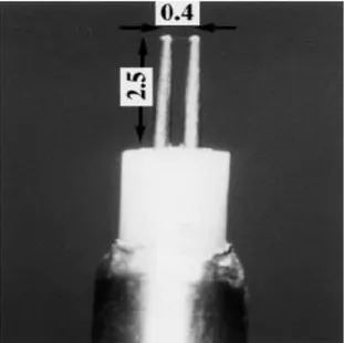
The wire is made of tungsten and has a length (lw) of 1 mm and a diameter (dw) of

2.5µm; it is held by two prongs 2 mm long.

Figure 3.16: Cold wires DAO121A, DAO123A

3.2.1.1 Calibration Process

The calibration in still air has been done in steady conditions: the cold wire and a thermocouple have been placed inside a metallic box which, in turn, have been put inside an oven (Fig. 3.17(a), Fig.17(b)). The electric cables of the probes come out of the oven through a hole which have been closed with red plasticine in order not to have heat dispersion (see Fig. 3.17(c) ).

DAO121A has been tested with 4R thermocouple; DAO123A has been tested with 2R thermocouple. The thermocouples have been linked to an amplifier in order to obtain significant values as output (in detail: thermocouple 4R was linked with TC amplifier TU4, thermocouple 2R was linked with TC amplifier TU7). For the calibration of these probes two cold wire boxes have been used: the black one (TUCW3) and the white one (TUCW2). These boxes basically consist in a Wheatstone bridge in which one of the four resistances is the cold wire, linked to the box by its input entries (Fig. 3.18).

(51)

31

(52)

32

Figure 3.18: (a) Schematic representation of the wiring of a cold wire; (b) power supplier.

The cold wire box is linked to a power supply (Fig. 3.18 (b)) which produces the desired value of voltage: for this test it has been set a value of ± 15V in order obtain a current inside the wire of around 0.2 mA. It’s important to have an electric current of small intensity in order to have a negligible Joule Effect. Through some BNC cables it was possible to read the output of the box (voltage of the bridge and current inside the wire) displayed in a multimeter.

For the calibration of the cold wire it has been chosen to set the range of temperatures between 20 and 90 °C with a ΔT of 10°C between two points. Before starting the test, the stability of the electronic setup has been tested monitoring the values of the cold wire and current outputs in function of time at ambient temperature. This is shown in Fig. 3.19: these data are relative to the white box TUCW2 and it can be noticed that they drift a bit.

Once the data relative to the current, cold wire and thermocouples outputs have been taken at ambient temperature, the oven is heated up to the prefixed target temperature. To obtain a stable value it took 1h40 minutes. The data have been registered up to 90°C degrees and the calibration was brought to an end in two days. As done for the calibration of thermocouples, also for the cold wires these data have been related with a linear trendline: using Excel it was possible to obtain

(53)

33

Figure 3.19: Stability of the white box TUCW2. The cold wire signal and the current supplied by the power

generator have been monitored at ambient temperature to test the stability of the Wheatstone bridge.

3.2.1.2 Wiring of the cold wires

Probe Head Electronics (input)

DAO123A 1A Black Box CH1

2A White Box CH1

DAO121A 1B Black Box CH2

2B White Box CH2

Table 3.3 Wiring of the cold wire transducers with the Wheatstone bridge entries.

-0,12 -0,1 -0,08 -0,06 -0,04 -0,02 0 0 10 20 30 40 50 Cold wire O u tp u t [V] TIme [min]

Cold wire output at ambient

temperature- White box

9,85 9,9 9,95 10 10,05 10,1 10,15 10,2 0 10 20 30 40 50 Volt age[ V] Time [min]

Voltage furnished by power supply at

ambient temperature- White box

(54)

34

3.2.1.3 Results

The following graphics (Fig. 3.20) are the calibration curves for the two probes.

Figure 3.20: Results of the static calibration in the oven of the two cold wires DAO121A , DAO123A

y = -0,05593x + 0,94313 R² = 0,99931 y = -0,09847884x + 1,87795631 R² = 0,99997421 -8 -7 -6 -5 -4 -3 -2 -1 0 0 20 40 60 80 100 Co ld w ir e o u tp u t [V} Temperature [°C]

TUCW2 (White Box) , 20-90 °C

2A 2B

y = 0,03341x - 0,71082 R² = 0,99923 y = 0,0308x - 0,7998 R² = 0,9996 -0,5 0 0,5 1 1,5 2 2,5 0 20 40 60 80 100 Cold wire o u tp u t [V] Temperature [°C]

(55)

35

3.2.2 Cold wire static calibration (heated jet)

The calibration in heated jet has been done using a more complicated setup. The cold wire has been tested always in static conditions registering its outputs at different Mach and temperature of an air jet.

For these tests the cold wire has been mounted on variable height support in order to put manually the probe inside and outside the heated jet setting the height of the support (Fig. 3.21). This support has been placed near a facility that blows the jet of air through a nozzle: changing the height of the support the head of the transducer was submerged into the flow. The facility for the heated jet was linked with a pipe to a heating system that, in turn, was linked to the air pressurised reservoir of the Von Karman Institute. The head of the probe was tested only for few seconds into the flow to preserve the wire which is extremely fragile: after having taken the data the support was moved manually to remove the probe from the jet.

The test consisted in measuring the output of the cold wire when inserted into a flow with known temperature and Mach conditions. At the same time pressure and temperature variations were registered with other probes. Before starting the test, the pressurized air reservoir was opened to reach a sufficient ΔP to get the desired Mach number.

Figure 3.21: Experimental setup for the static calibration of the cold wire in the jet; it is visible the metallic

(56)

36

3.2.2.1 Experimental Setup

The cold wires have been linked to the Wheatstone bridge as done in the calibration in the oven: the tested transducer has been linked to the input of the box used as Wheatstone bridge (Fig. 3.22); this box, in turn, has been connected to a power supply and to a multimeter in order to read the output of the probe. The pressurized air has been blown through a nozzle. Inside the nozzle it has been placed a differential pressure transducer (SENSYM) and a thermocouple (2R): the latter has been linked to an amplifier in order to obtain significant values. Outside the nozzle, through some rigid supports it has been installed the second thermocouple (4R, connected to an amplifier) while the cold wire has been mounted on a variable height support, as mentioned before.

The connections of the heads of the probes with the Wheatstone bridge (black/white boxes) are the same used for the calibration in the oven.

(57)

37

3.2.2.2 Pressure Readings

A differential pressure transducer (SENSYM, R4S4) has been inserted inside the nozzle in a way to get differential pressure readings. Before using the probe in the static test the transducer has been calibrated: one head of the probe has been connected inside the sealed case of the pressure calibrator through a thin plastic pipe while the other was kept to ambient pressure (Fig. 3.23). The transducer has been linked with a power supply through a connector: through a multimeter it was possible to read the electrical output of the probe.

Figure 3.23: Setup for the calibration of the SENSYM (differential pressure transducer)

The pressure calibrator output was set initially to zero. Once the sealed chamber was closed it was possible to add or subtract pressure to one side of the transducer (the other side being at constant ambient pressure) with the handles of the instrument. As done for the calibration of thermocouples also in this case several points of pressure-voltage have been taken and have been inserted in Excel in order to get a linear trend with values of slope and intercept. As can be seen in the

(58)

38 Figure 3.24: Calibration curve of the SENSYM R4S4

3.2.2.3 Temperature Readings

Two temperature probes have been installed in the facility to get more details on the evolution of temperature. The 2R thermocouple was mounted inside the nozzle and linked to the TC amplifier TU7; the 4R thermocouple was mounted with a rigid support right at the exit of the nozzle and linked to the TC amplifier

TU4. In Fig. 3.25 we can see that the head of the thermocouple 4R is closely

placed near one of the two heads of the cold wire.

Other two thermocouples have been installed inside the heating system (Fig. 3.26).

Figure 3.25: Thermocouple 4R (up) and cold wire (put horizontally).

y = 3,34675550x - 0,37742555 R² = 0,99999870 0,0000 1,0000 2,0000 3,0000 4,0000 5,0000 0,8000 0,9000 1,0000 1,1000 1,2000 1,3000 Vo ltage [V] P [bar]

(59)

39

Figure 3.26: The heating system for the air pressurized reservoir. It is provided with two thermocouples to

monitor the temperature before the air reach the nozzle.

3.2.2.4 Setting Mach number

The tests in the heated jet have been done using several Mach numbers. The desired value has been reached using air pressurized into a reservoir.

The data of ambient pressure came from the server of Von Karman Institute. Knowing the value of Mach number required for the test and the ambient pressure it was possible to obtain the required total pressure using equation (3.25)

𝑃𝑡𝑜𝑡 𝑃_𝑠 = [1 + ( 𝛾 − 1 2 ) 𝑀 2_] 𝛾 𝛾−1 (3.25)

Being 𝑃𝑠 the ambient pressure and 𝑘 the specific heat ratio of air. The air has been

considered a perfect gas, having 𝛾 = 1.4, specific heat at constant pressure 𝐶_𝑝 =

1.005 𝐾𝐽

𝐾𝑔 𝐾 and specific constant 𝑅 = 287.05

𝐽 𝐾𝑔 𝐾 .

The dynamic pressure dP stems from the difference from the total and static

pressure (𝑃_𝑎𝑚𝑏) :