A Knowledge Flow as a Software Product Line

(1)

ALMA MATER STUDIORUM - UNIVERSITA' DI BOLOGNA

CAMPUS DI CESENA

SCUOLA DI INGEGNERIA E ARCHITETTURA

CORSO DI LAUREA MAGISTRALE IN INGEGNERIA E SCIENZE

INFORMATICHE

TITOLO DELLA TESI

A KNOWLEDGE FLOW AS A SOFTWARE PRODUCT LINE

Tesi in:

INTELLIGENZA ARTIFICIALE

Relatore:

Presentata da:

Prof. Vittorio Maniezzo

Luca Parisi

Sessione II

(2)

(3)

Abstract

Constructing a data mining workflow depends at least on the collected dataset and the objectives of users. This task is complex because of the increasing number of available algorithms and the difficulty in choosing the suitable and parametrized algorithms. More-over, in order to decide which algorithm has the best performances, data scientists often need to use analysis tools to compare performances of different algorithms. The purpose of this project is to lay the foundations of a software system that leads the construction of such workflows into the right direction toward the best ones.

(4)

(5)

Acknowledgements

The research presented in this thesis has been done during my Erasmus+ experience in the university of Nice-Sophia Antipolis in the I3S Laboratory, Sophia Antipolis, France. First of all, I would like to thank my french academic supervisors, Prof. Frédéric Precioso and Prof. Mireille Blay Fornarino, by accepting me, as intern, to work on this research. They helped me constantly during my research and they explained me how to work as a researcher. I would like to thank also the engineer that worked and currently is working on the project ROCKFlows, Cécile Camilleri. She is the critical eye that every research team should have: she reviewed a lot of times my work and the results found, by ad-vising me what could be improved or was not clear. Furthermore, she taught me some engineer programming skills which I was not used to apply before. Always related to this research, I would like to thank my italian academic supervisor, Vittorio Maniezzo. His course of Artificial Intelligence taught me everything I needed to know in order to face this research, from predicate logic to the statistical hypothesis testing to the explanation of some algorithms of regression and classification. Without his course, I would not have had the necessary basics in order to face this research. Finally, I would like to thank my family, who allowed me to live this magnificent experience, which made me improve a lot both as a person and as a student. It is thanks to this experience that I’ve improved my english and learnt both french and spanish with my french and spanish friends. Further-more, I discovered that I love traveling and learn new languages, which is something that I did not know before. Lastly, I would like to thank my friends, who distracted me from the high pressure coming from the studies.

Thank you everyone,

(6)

(7)

List of Figures

1.1 General Supervised Classiﬁcation Workﬂow . . . 3

1.2 Weka’s Knowledge Flow . . . 6

1.3 Microsoft Azure Cheat Sheet . . . 7

1.4 GUI of ROCKFlows . . . 7

5.1 Linear Dependency, time of execution of (p11, Svm) . . . 46

5.2 Linear Dependency, time of execution of (p11, Bagging LWL) . . . 46

5.3 Logarithmic Dependency, memory usage of (p11, NBTree) . . . 47

5.4 Linear Dependency, memory usage of (p11, Bagging LWL) . . . 47

A.1 Simpliﬁed Feature Model ROCKFlows . . . 57

(10)

List of Tables

1.1 Subset of Iris Dataset . . . 2

3.1 List of 101 Datasets . . . 18

3.2 Domain of Applicability of Pre-processing . . . 22

3.3 Part of Collected Performances, Adult p0 . . . 27

3.4 Part of Ranking of Workﬂows, Adult . . . 29

4.1 Evaluation Impact . . . 32

4.2 Pre-processing Impact, 4-Fold cross-validation . . . 33

4.3 Pre-processing Impact, 10-Fold cross-validation . . . 33

4.4 Missing Value Impact, 4-Fold cross-validation . . . 36

4.5 Missing Value Impact, 10-Fold cross-validation . . . 36

5.1 Data pattern, 4-Fold cross-validation . . . 39

5.2 Data pattern, 10-Fold cross-validation . . . 39

5.3 Number of Classes Impact, mushrooms vs pendigits . . . 40

5.4 Number of Instances Impact . . . 41

5.5 Number of Attributes Impact, waveform vs waveform-noise . . . 43

5.6 Number of Attributes Impact, Adult p10 vs Adult p5 . . . 43

A.1 Parent-Child primitives of Feature Model . . . 54

A.2 Cross-Tree primitives of Feature Model . . . 54

A.3 Example of not knowledge . . . 55

(11)

List of Algorithms

(12)

(13)

Chapter 1: Introduction

1.1 Supervised Classiﬁcation

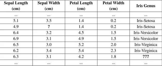
Mobile sensors and social networks are only a few examples of applications that gen-erate a huge amount of data each day. Such a collected big data can be analysed and new valuable knowledge can be extracted from it. The overall goal of data mining is to extract valuable information from datasets in order to retrieve new knowledge for further use. In the data mining field there exist several problems, one of which is the supervised classification problem. In order to explain better what supervised classification means, Table 1.1 reports an extract of the Iris dataset. Iris is a genus of one flowering plant, and its genus is defined according to the sepal length, sepal width, petal length and petal width of each flower. In the Iris dataset, each flower is one row of the dataset. In this example, there are three genuses: Iris-setosa, Iris-versicolor and Iris-virginica. In the first six rows of the dataset the Iris genus is known, but in the last one it is unknown. The goal of classification is to predict the right Iris genus for each flower where we do not know its genus, in this case the last row of the dataset. Predictions are made by a classification algorithm. Supervised classification means that before predicting the Iris genus, the clas-sification algorithm needs to learn some rule from the flowers with a known Iris genus. That is, the algorithm needs to be trained in order to build a model that knows how to predict the Iris genus. Let K be the subset of the flowers with a known Iris Genus, in this example the first six rows of the dataset. Once we choose a classification algorithm and we build a model that is able to predict the Iris genus, how can we know if the predicted genuses are the correct ones? We need to evaluate whether the predictions done by the model are good or not. We can check the performances of the model by making it predict the Iris genuses of the flowers that we already know. To this purpose, we divide K in two datasets, K1 and K2, such that K1∩ K2= /0 and K1∪ K2=K. K1 is the training set, and

it is used to train the classiﬁcation algorithm and to build the model, while K2 is the test

set, and it is used check if the predictions done by the training model correspond with the acutal Iris genus of the ﬂower. In order to check the performances of the model, we can calculate the accuracy, which is the percentage of correct predicted instances of the test set. After the evaluation, if the accuracy obtained by the model is good, the same model can be used to predict the Iris genus of the ﬂowers with an unknown genus. Otherwise, we should build a different model that leads to a better accuracy during the evaluation of the model.

(14)

1. Introduction Sepal Length (cm) Sepal Width (cm) Petal Length (cm) Petal Width (cm) Iris Genus ... ... ... ... ... 5.1 3.5 1.4 0.2 Iris-Setosa 4.9 ? 1.4 0.2 Iris-Setosa 6.4 3.2 4.5 1.5 Iris-Versicolor 6.9 3.1 4.9 1.5 Iris-Versicolor 6.5 3.0 5.2 2.0 Iris-Virginica 6.2 3.4 5.4 2.3 Iris-Virginica 6.3 3.1 4.2 1.8 ??? ... ... ... ... ...

Table 1.1: Subset of Iris Dataset

1.1.1 Vocabulary

This section aims to define well the terminology used in this report to refer to clas-sification problems. For non-data scientist readers, it may be not so easy to understand fully the concepts illustrated here if they do not know the proper terminology. Further-more, different terminologies are used in other books or articles, so sometimes it is hard to understand well the content of an article if the terminology is not well specified. The Iris dataset shown in Table 1.1 is used as an example dataset. The terminology used in this report can be summarized in the following terms:

• Instance: each row of the dataset is one instance.

• Attribute: each column of the dataset is one attribute. Examples of attributes are: ”sepal length”, ”sepal width”, ”petal length”, ”petal width” and ”Iris genus”. • Missing Value: each instance contains one value for each attribute. If, for any

attribute, the value is not known, it is a missing value. An example of a missing value is the value ”sepal width” of the second instance.

• Numeric Attribute: one attribute is numeric if it contains only numeric values. Ex-amples of numeric attributes are ”sepal length”, ”sepal width”, ”petal length” and ”petal width” are numeric attributes.

• Nominal Attribute: one attribute is nominal if it contains only categories (text val-ues). ”Iris genus” is an example of nominal attribute.

(15)

1. Introduction

Figure 1.1: General Supervised Classiﬁcation Workﬂow

• Class Attribute: it is one attribute of the dataset that identiﬁes the class of each instance. In the classiﬁcation problems, the class attribute must be nominal, it cannot be numeric. In the Iris dataset, the class attribute is ”Iris genus”.

• Class Label: each instance contains one class label, which is the value of the class attribute. An example of class label is ”Iris-Setosa”.

• Multi-Class vs Binary-Class Problem: If the class attribute contains more than two distinct categories, the classiﬁcation problem is a multi-class problem. Otherwise, it is a binary class problem (called also two-class problem).

• Classiﬁer: synonym of ”classiﬁcation algorithm”.

1.1.2 Supervised Classiﬁcation Workﬂows

A supervised classification process can be defined as a workflow of phases, as shown in Figure 1.1. An optional pre-processing to apply to the dataset is the first phase. The purpose of pre-processing is either to make the dataset compatible with the classification algorithm that we want to apply on it, or to modify the data in order to expect better accuracies when predicting classes. Typical pre-processing techniques are:

• Data Selection: only the relevant attributes are selected from the dataset.

• Data Cleaning: for example, if the dataset contains some missing values and the chosen classiﬁer cannot deal with missing values, we need to replace them with another value.

(16)

1. Introduction

• Data Transformation: the original data is transformed into a different kind of data. For example, numeric attributes may be discretized into nominal attributes, or trans-formed into a different scale, etc...

After the pre-processing phase, we need to choose a classification algorithm to apply on the pre-processed dataset. In the data mining literature there exist a lot of classifi-cation algorithms, each one with different performances. Some algorithms have some parameters to be set, and different values assigned to these parameters may change the performances of the classification algorithm. The last phase of the workflow is the evalu-ation of results. Once we have defined a pre-processing technique, chosen a classifier and set its parameters, we want to test whether the workflow will lead to good performances or not with an evaluation method. The simplest evaluation method is to train the classifier on one training set, to test it on one test set, and to calculate the accuracy obtained as performance indicator. Anyway, the accuracy obtained on only one test set may not be a good performance indicator, because it may not represent well the future instances to be predicted. In order to have an evaluation more statistically sound, we may train and test the classifier on several training sets and test sets. An evaluation method that does this is the N-fold cross validation, which evaluates for N times a classifier on different training sets and test sets. Let K be the dataset used in the evaluation phase, where in each instance the class label is known. Then, K is divided into N folds, K1,K2, ...,KN,

and for N times, (N-1) folds are used as training set and 1 fold is used as test set. The ﬁnal accuracy is the average of the N accuracies found on each of the N test sets. If the accuracy obtained during the evaluation is good enough, the evaluated model can be used to predict future instances with unknown class labels, otherwise it should be changed. There are three ways to change the workﬂow:

1. change the pre-processing technique applied to the original dataset 2. choose a different classiﬁer

3. set different values to the parameter

Each one of these changes leads to a different workﬂow that can obtain better or worse accuracies in the evaluation phase.

1.2 Motivations

When there is a classiﬁcation problem to be solved, data scientists, according to their knowledge and to their experience, know the best practices that solve it the best. They

(17)

1. Introduction

know how to manipulate the problem and which algorithms will probably lead to the best results. On the other hand, non-expert users neither know the best practices nor have any experience in the data mining field. Both for data scientists and non-expert users, there exist a lot of platforms that help them in building workflows. Section 1.2.1 reports the state of the art of such existing systems. Currently, we are implementing a system that leads users into the right direction in finding their most suitable workflow, depending on the problem to be solved. Section 1.2.2 reports the differences among the existing platforms and the system that we are implementing, called ROCKFlows1_.

1.2.1 State Of The Art

Data scientists can use platforms like Weka [6], Orange [10], KNIME [11], Rapid-Miner [12] and ClowdFlows [14] [15], in order to build workflows more easily. On these platforms, users can create and execute workflows by selecting a set of components and by connecting them. Figure 1.2 shows an example of a workflow built on Weka’s knowl-edge flow, which allows to build workflows by dragging and dropping components on the screen and to connect them easily by using arrows.

Although such platforms are useful for data scientists, they may be a little bit com-plex for non-expert users. For them, it may be more helpful a system that either solves automatically the problem, or advise a set of suitable workflows to use, or suggests the components to select. Big companies have proposed their own cloud platforms, which aim to be such a system. The IBM Watson platform [18] offers an interface to analyze unstructured data (such as text files) and take as input questions in plain English. Then, the system presents answers to the questions submitted by analyzing automatically the dataset given by the user. Amazon’s product [17] is a black box similar to the IBM’s platform, but it is focused on supervised classification and regression problems. The workflow is built and executed automatically by the platform, and minimal responsibil-ity for the choice of the workflow is left to the users. On the other hand, the solution proposed by Microsoft Azure [16] is different both from IBM’s and from Amazon’s plat-form. Instead of finding the solution automatically for users, it gives them advices on which components to select, based on the known machine-learning best practices. Figure 1.3 shows the Microsoft cheat sheet that orients users in choosing the proper classification algorithm, in case of two-class classification problems.

Finally, there exists a system born in the academic world, named MLBase [13]. It aims to free users from the algorithm choice by building a sophisticated cost-based model. It provides early answers to the users, then it keeps working in background while users use

(18)

1. Introduction

Figure 1.2: Example of a Workﬂow built on Weka’s Knowledge Flow.

the system, in order to optimize and to improve the workﬂow.

1.2.2 ROCKFlows Features

ROCKFlows aims to lay the foundations of a system intended both to data scientists and to non-expert users. Data scientists are free to build their desired workflows, while non-expert users can ask the system to select automatically components of the workflow. For example, if data scientists want to use a specific algorithm, they are free to choose it. Similarly, if non-expert users do not know which algorithm is better to use, the system will select one of the most suitable algorithm depending on their dataset. With respect to the Weka knoledge flow (Figure 1.2), users do not need to select and to connect the components with arrows. Once the components are selected, ROCKFlows knows how to connect them and how to build the workflow. Similar to the IBM Watson platform, ROCKFlows asks users questions in plain english, and they answer by choosing one on the available pre-built answers. Figure 1.4 reports an example of questions / answers

(19)

1. Introduction

Figure 1.3: Microsoft Azure cheat sheet that orients users in choosing the proper classiﬁcation algorithm, in case of two-class classiﬁcation problems

Figure 1.4: GUI of ROCKFlows: questions are asked in plain english, and users answer by selecting pre-built answers

asked by the GUI of ROCKFlows.

With respect to the solution proposed by Microsoft Azure (Figure 1.3), ROCKFlows aims to consider workflows which does not correspond necessarily to knwon best prac-tices. Our purpose is to explore more the space of the solutions of machine learning workflows. For example, in the two-class classification problem, Microsoft Azure advise only nine algorithms, depending on the dataset properties, on the speed of training and on the level of accuracy that users want. Finally, with respect to MLBase, the objective of ROCKFlows is not to keep working in background in order to improve the workflows advised to the users. ROCKFlows aims to predict right away the most suitable workflows,

(20)

1. Introduction

without comparing all the possible workﬂows in background in order to ﬁnd the best one.

1.3 Goals Of The Internship

The work done for this internship is the theoretical research that there is behind ROCKFlows. For starters, we face only the supervised classification problem. The main goal of this internship is to define a strategy that let ROCKFlows predict right away the most suitable workflows to the users, without comparing the performances of different workflows as the Amazon or MLBase solutions do. To reach this goal, ROCKFlows needs to know in advance the performances that workflows will have on the user’s dataset, that is, it should be able to skip the evaluation phase. From users’ point of view, the most suitable workflow can be either the one who reaches the best accuracy on their datasets, or the one who reaches a good accuracy by respecting, in the same time, some users’ con-straints. Users’ constraints may concern the performances of the execution of workflows, for example, the total time of execution of workflows or the amount of RAM occupied by the process executing the workflow. To this purpose, the second goal of this internship is to predict both the time of execution of a workflow and the memory used by the process executing it, depending on the user’s dataset.

1.4 Challenges

As explained in Section 1.1.2, when we build a classiﬁcation workﬂow we need to choose at least three components:

• An optional pre-processing technique to apply to the dataset • A classiﬁcation algorithm to choose

• The values for the parameters requested by the classiﬁer

The first challenge of this internship is the high variability coming from the construc-tion of workflows. Each modificaconstruc-tion to one of these three components leads to a different workflow. So, even if we would like to compare all the possible workflows among them in order to find the most suitable for the user, it would be impossible because of the huge time that we should wait. This is also one of the hot topic research in the data mining field. In terms of accuracy, predictions of workflows would be easier if, among all the classification algorithms that exist in the literature, only one of them had always better

(21)

1. Introduction

accuracies than the others. That is, the construction of workflows would be easier if we had to select only one classifier because it is always the best regardless the users’ datasets. Unfortunately, the No-Free-Lunch Theorem [2] states that the best classifier will not be the same for each dataset. The same holds for the pre-processing choice. The applica-tion of a pre-processing technique on the user’s dataset changes the performances of the algorithms of classification, and in the data mining literature there does not exist one pre-processing technique that guarantees always the best performances than the others. The second challenge of this project is to know in advance the performances that workflows will have during their execution, without doing the evaluation phase. That is:

• How can we predict the accuracy that a workﬂow will have on users datasets, without doing the evaluation phase?

• How can we predict the total time of execution that a workﬂow will have on users datasets, without doing the evaluation phase?

• How can we predict the memory usage that the process executing the workﬂow will have on users datasets, without doing the evaluation phase?

(22)

(23)

Chapter 2: Related Work

The most related work to the research done for this internship is the paper written by M.F.Delgado et al. (2014): Do we Need Hundreds of Classifiers to Solve Real World Classification Problems? Journal of Machine Learning Research 15 3133-3181. This paper does not consider all the phases of a general workflow as we do in this project, it is focused on the choice of the best classification algorithm for solving supervised classification problems. In order to know which classifiers work best in general, the authors have tested 179 classifiers on 121 datasets, of which 117 coming from the UCI repository [5]. About the 179 classifiers, they have tested the implementation of the same algorithms done on different frameworks, such as R [7], Weka [6], C and Matlab (by using the Neural Network Toolbox) [8].

Regarding the pre-processing, they have applied the same pre-processing to each dataset. At ﬁrst they have converted all the nominal attributes into numeric attributes by using a simple quantization: if a nominal attribute x may take discrete values {v1, ...,vn}

when it takes the discrete value viit is converted to the numeric value i ∈ {1,...,n}. Then,

they have standardized each attribute, so in the end each attribute is numeric, where its mean is equal to zero and its standard deviation is equal to one. Finally, they have re-placed all the missing values with the value 0. Apart from these operations, they have not done any further pre-processing. For each classifier, the authors have reported the values assigned to its parameters. Anyway, some parameters need to be tuned on the specific dataset before being assigned. In this case, the authors have tuned them on a validation dataset, which is extracted by each of the tested dataset before evaluating the algorithm. The validation dataset is formed by one training set and by one test set. The training set contains the 50% of the total number of instances of the dataset, while the test set con-tains the remaining 50%. About the datasets of the UCI repository [5], some of them are already separated in one training set and one test set, while others are defined in a unique file. For the evaluation phase, the authors have decided to use two different evaluation methods. If the dataset is defined in a unique file, the classifier (with the tuned parameter values) is evaluated with a 4-fold cross validation, otherwise, it is trained on the given training set and tested on the given test set.

As results of the paper, the authors have reported a final ranking of the 179 classifiers, where for each classifier they have calculated the Friedman rank [3], the average accuracy obtained on the 121 datasets and the Cohen k [4] as performance indicators. From their experiments, the authors have found that the algorithm that obtained the best results is Random Forest implemented in R and accessed via caret, which achieves 94.1% of the maximum accuracy, while the second best one is the SVM with Gaussian kernel imple-mented in C using LibSVM, which achieves 92.3% of the maximum accuracy. As

(24)

conclu-2. Related Work

sion, they have compared the families of classifiers. They say that random forest is clearly the best family of classifiers (3 out of 5 bests classifiers are RF), followed by SVM (4 clas-sifiers in the top-10), neural networks (5 members in the top-20) and boosting ensembles (3 members in the top-20). In order to make the experiments reproducible, the authors have made their 121 pre-processed datasets available for download1_{. Furthermore, for}

each dataset, they have also published two files: conxuntos.dat defines the validation dataset used for the parameter tuning of the algorithms, while conxuntos kfold.dat defines the folds used by the 4-fold cross validation.

2.1 Critics

The results reported into the paper are very interesting and show that, generally, there are some families of classifiers that work better than the others. Since in general we ob-tain good performances with the Random Forest or Svm families of classifiers, we could base the choice of the classification algorithm only by considering these two families of classifiers. Anyway, their experiments present five points that may change the results reported by the authors:

1. In the evaluation phase, they use two different evaluation methods in order to cal-culate the same final ranking of classifiers. If the choice of the evaluation method affects the results of the evaluation, it will affect also the final ranking of the clas-sifiers reported by the authors. For example, the authors could have obtained a different ranking of classifiers if they had used the 4-Fold cross validation method also on the datasets already separated into one training set and one test set. So, the first critic can be expressed by the following questions: What is the impact of the evaluation method used for the evaluation phase? Can we find significant dif-ferences in the final ranking of classifiers if we consider two different evaluation methods?

2. They perform only one pre-processing technique, because they say: the impact of these transforms can be expected to be similar for all the classifiers; however, our objective is not to achieve the best possible performance for each data set (which eventually might require further pre-processing), but to compare classifiers on each set. The second critic can be expressed by the following questions: What if the impact of the pre-processing is not similar for all the classifiers? Can we find

1_{http://persoal.citius.usc.es/manuel.fernandez.delgado/papers/jmlr/data.tar.gz}

(25)

2. Related Work

signiﬁcant differences in the ﬁnal ranking if we consider also other pre-processing techniques?

3. Some Weka classifiers cannot work directly on the pre-processed datasets made by the authors, because they can work only on nominal attributes. In this case, Weka converts automatically the numeric attributes into nominal attributes in order to make the dataset suitable for these classifiers. The Weka classifiers that can work only on nominal attributes are the following:

• weka.classiﬁers.bayes.BayesNet • weka.classiﬁers.rules.OneR

• weka.classiﬁers.meta.Bagging OneR • weka.classiﬁers.meta.MultiBoostAB OneR

The consequence of this is that the results obtained by these classifiers refer to datasets different from the ones used by the authors, so maybe the final ranking of classifiers has been affected by this. As we wondered in the previous critic, if the impact of pre-processing is significant, we might find a different final ranking if we test the classifiers that can work also on numeric attributes on the dataset pre-processed by Weka that contain only nominal attributes.

4. In the pre-processing technique used by the authors, they have replaced the missing values with the value 0. Anyway, some algorithms can manage missing values, so for them it is not necessary to replace them. So, the third critic can be expressed by the following questions:What is the impact of missing values on these algorithms? Can we find significant differences in the ranking for the classifiers that can manage missing values, if we do not replace them?

5. They have tested some meta-classifiers implemented in Weka with the default base classifier, the zeroR classifier [?]. This classifier always predicts the mode of the nominal attributes, that is, in case of the class labels, it predicts always the most frequent class of the dataset. This is the reason why in the final ranking reported into the paper, the following meta-classifiers have bad results:

• weka.classifiers.meta.Grading • weka.classifiers.meta.MultiScheme • weka.classifiers.meta.Vote

(26)

2. Related Work

• weka.classifiers.meta.Stacking: the authors use the stacking ensemble method only with one zeroR base classifier, while the method is intended to test sev-eral base classifiers, not only one.

• weka.classiﬁers.meta.StackingC: the same reason as Stacking.

(27)

Chapter 3: Strategy of Research

In order to skip the evaluation phase and to predict the best workflows on untested datasets, ROCKFlows needs to know at least what their performances are on some datasets. Basing on the information retrieved, we can find some rules that allow the system to pre-dict the performances of the workflows on untested datasets, without doing the evaluation phase. To this purpose, we have defined a strategy that can be summarized in four phases: 1. Experiments (Section 3.1): each workflow is tested on some datasets and its

perfor-mances are retrieved and stored in Excel ﬁles.

2. Analysis (Section 3.2): we analyse how much the accuracy obtained by the work-ﬂows on each dataset is good, without considering only the average accuracy as value of comparison.

3. Significant Impacts on Classifier Performances (Chapter 4): by using the Analysis phase, we study which factors have a significant impact on the performances among different workflows. By replicating partially the experiments done by Delgado et al. (Section 2), we want to find an answer to the questions presented in critics #1, #2 and #4 of Section 2.1.

4. Predictions (Chapter 5): by exploiting the results retrieved in the Analysis phase (Section 5.1), we want to find some rules that allow to predict the performances of workflows on untested datasets, without doing the evaluation phase. Hence, we can predict the workflows that, allegedly, will reach the best accuracy (Section 5.1) on untested datasets. Similarly, we want to predict the total time of execution of each workflow and the memory usage of the process executing it (Sections 5.2 and 5.3).

3.1 Experiments

The research done for this internship is based on the experiments reported in Section 2. We have replicated in part the experiments of Delgado et al., but we have limited our experiments on the Weka’s platform (version 3.6.14), by testing 65/179 classifiers imple-mented with the Weka’s APIs on 101/121 datasets of the UCI repository [5]. Anyway, since this project is focused on workflows and not only in classifiers, we have extended the experiments done by the authors by considering 12 pre-processing techniques along with the original dataset (without pre-processing). For each algorithm we have set the same parameters reported by the authors, hence, except for the parameters of the classi-fier LibSvm, we do not tune the parameters before testing the classiclassi-fier on each dataset. Hence, we define a workflow as a 2-tuple (pi,cj) composed by:

(28)

3. Strategy of Research

• p: the choice of a sequence of pre-processing techniques applied to the dataset • c: the choice of the algorithm of classiﬁcation

Any variation to pior to cj deﬁnes a different workﬂow that the system may take into

account when predicting the best workﬂow to the users. For research sake reproducibility, we have made available the code used to do the experiments.1

3.1.1 Datasets (D)

In our experiments, we have tested 101/121 datasets coming from the UCI repository [5]. In the rest of this report, the set of 101 datasets is referred as D.

Since we based our experiments on Weka’s platform, we have deﬁned each dataset dk∈ D in .arff ﬁles, which is the format used by Weka to read them. In the UCI repository,

for each dataset is given its raw data and the description of the problem, which explains what each attribute refers to. Generally, each nominal attribute is represented with a range of numbers, where each number refers to a specific category. For example, an attribute Size that have categories small, medium, large can be expressed as three numbers: 0,1,2 }. Since datasets in the UCI repository are not in the .arff format, we had to define manually the categories for each nominal attribute. Likewise, we have set a numeric attribute only when its values are real numbers, for example, the measure coming from a sensor. In our experiments, the difference between numeric and nominal attributes is very important because the nature of the attributes of the dataset defines which pre-processing techniques are applicable on them, as explained in Section 3.1.2. Moreover, from the description of datasets, we have removed all the instance identifiers, that is, all the attributes that present a unique value for each instance. We have done this manual pre-processing because the identifiers may affect the results obtained by the experiments.

Dataset Properties

Furthermore, in our experiments it is important to know the structure of the datasets, which we identify with the following properties:

• Number of Attributes • Number of Instances

• Number of Classes: 2 (binary-class problem) or more (multi-class problems)

1_{https://github.com/ROCKFlows/experiments-public/tree/master/sourceCode}

(29)

• Type of Attributes: nominal, numeric or both of them. • Missing Values: Does the dataset contain any missing value?

Dataset List

Table 3.1 shows the set of datasets D used in our experiments, along with the prop-erties of each dataset. For reproducible research sake, we have made the 101 datasets available for public download.2

3.1.2 Pre-Processing (P )

From each dataset dk∈ D to test, several pre-processed datasets with different

proper-ties are created by applying a set of pre-processing techniques P to dk. In our experiments,

we have decided to test the original dataset along with 12 pre-processing techniques, that is, from 1 to 12 pre-processed datasets may be created from the original one, depending on if the pre-processing technique pi∈ P is applicable to the original dataset (Section

3.1.2). Each pre-processing technique pi∈ P may contain one or more operations, in

this case they are applied sequentially to the original dataset. The set of pre-processing techniques P used in our experiments is reported in the following:

p0 No pre-processing (original dataset)

p1 {Discretize}

p2 {Replace Missing Values}

p3 {Replace Missing Values, Discretize}

p4 {Nominal To Binary}

p5 {Replace Missing Values, Nominal To Binary}

p6 {Attribute Selection}

p7 {Discretize, Attribute Selection}

p8 {Replace Missing Values, Discretize, Attribute Selection}

p9 {Nominal To Binary, Attribute Selection}

2_{https://github.com/ROCKFlows/experiments-public/tree/master/Resources/}

(30)

Dataset #Att. #Inst. #Cls. Att. Types M.V.

ac-inﬂam 6 120 2 Both no

ac-nephritis 6 120 2 Both no

adult 14 32561 2 Both yes

annealing 38 798 6 Both yes

arrhythmia 279 472 16 Both yes

audiology-std 69 171 18 Nominal yes

balance-scale 4 625 3 Numeric no

balloons 4 16 2 Nominal no

bank 16 4521 2 Both no

blood 4 748 2 Numeric no

breast-cancer 9 286 2 Nominal yes

bc-wisc 8 699 2 Nominal yes

bc-wisc-diag 29 569 2 Numeric no

bc-wisc-prog 32 198 2 Numeric yes

breast-tissue 9 106 6 Numeric no

car 6 1728 4 Nominal no

ctg-3classes 45 2126 3 Numeric yes

chess-krvkp 36 3196 2 Nominal no

congress-voting 16 435 2 Nominal yes

conn-bench-sonar 60 208 2 Numeric no

conn-bench-vowel 12 528 11 Both no

contrac 9 1473 3 Both no

credit-approval 15 690 2 Both yes

cylinder-bands 37 512 2 Both yes

dermatology 34 366 6 Both yes

echocardiogram 12 131 2 Both yes

ecoli 7 336 8 Numeric no fertility 9 100 2 Numeric no ﬂags 28 194 8 Both no glass 9 214 7 Numeric no haberman-survival 3 306 2 Both no hayes-roth 4 132 3 Numeric no

heart-cleveland 13 303 5 Both yes

heart-hungarian 13 294 2 Numeric yes

heart-switzerland 13 123 5 Numeric yes

Table 3.1: List of 101 tested datasets coming from the UCI repository. M.V. stands for ”Missing Values”

(31)

heart-va 13 200 5 Numeric yes

hepatitis 19 155 2 Both yes

hill-valley 100 606 2 Numeric no

horse-colic 22 300 2 Both yes

ilpd-indian-liver 10 583 2 Both no image-segmentation 19 210 7 Numeric no ionosphere 34 351 2 Numeric no iris 4 150 3 Numeric no led-display 7 1000 10 Nominal no lenses 4 24 3 Nominal no libras 90 360 15 Numeric no low-res-spect 101 531 9 Numeric no

lung-cancer 56 32 3 Nominal yes

lymphography 18 148 4 Both no magic 10 19020 2 Numeric no mammographic 5 961 2 Numeric no molec-biol-promoter 57 106 2 Nominal no monks-1 6 124 2 Nominal no monks-2 6 169 2 Nominal no monks-3 6 122 2 Nominal no

mushroom 22 8124 2 Nominal yes

musk-1 166 476 2 Numeric no

musk-2 166 6598 2 Numeric no

nursery 8 12960 5 Nominal no

ozone 72 2536 2 Numeric yes

page-blocks 10 5473 5 Numeric no

parkinsons 22 195 2 Numeric no

pendigits 16 7494 10 Numeric no

pima 8 768 2 Numeric no

pb-MATERIAL 11 107 3 Both yes

pb-REL-L 11 107 3 Both yes

pb-SPAN 11 107 3 Both yes

pb-T-OR-D 11 107 2 Both yes

pb-TYPE 11 107 6 Both yes

planning 12 182 2 Numeric no

(32)

post-operative 8 90 3 Nominal yes

primary-tumor 17 330 15 Nominal yes

ringnorm 20 7400 2 Numeric no seeds 7 210 3 Numeric no spambase 57 4601 2 Numeric no spect 22 80 2 Nominal no spectf 44 80 2 Numeric no st-aust-cred 14 690 2 Both no st-germ-cred 20 1000 2 Both no st-heart 13 270 2 Numeric no st-landsat 36 4435 6 Numeric no st-shuttle 9 43500 7 Numeric no st-vehicle 18 846 4 Numeric no steel-plates 27 1941 7 Numeric no synth-ctrl 60 600 6 Numeric no teaching 5 151 3 Both no thyroid 21 3772 3 Both no tic-tac-toe 9 958 2 Nominal no titanic 3 2201 2 Nominal no

trains 32 10 2 Nominal yes

twonorm 20 7400 2 Numeric no vc-2classes 6 310 2 Numeric no vc-3classes 6 310 3 Numeric no wall-following 24 5456 4 Numeric no waveform 21 5000 3 Numeric no waveform-noise 40 5000 3 Numeric no wine 13 179 3 Numeric no wine-qual-red 11 1599 11 Numeric no wine-qual-white 11 4898 11 Numeric no yeast 8 1484 10 Numeric no zoo 16 101 7 Nominal no Continuation of Table 3.1

p10 {Replace Missing Values, Nominal To Binary, Attribute Selection}

(33)

p11 The same pre-processing described in Section 2 (we have taken directly the dataset

released by the authors)

p12 We apply pre-processing p6to the pre-processed dataset p11

In the rest of this report, each pre-processed dataset is identiﬁed with the same iden-tiﬁer of the above processing techniques. For example, we can refer to ”the pre-processed dataset p4” in order to specify the pre-processed dataset obtained after applying

the pre-processing technique p4to the original dataset.

Pre-processing {pi∈ P : 1 ≤ i ≤ 10} are based on four Weka ﬁlters:

• weka.filters.unsupervised.attribute.ReplaceMissingValues: replaces missing values with the mean (if the attribute is numeric) or the mode (if the at-tribute is nominal)

• weka.filters.unsupervised.attribute.Discretize: discretizes, by simple binning, a numeric attribute into a nominal attribute. The maximum number of bins is 10.

• weka.filters.unsupervised.attribute.NominalToBinary: converts a nom-inal attribute into a set of binary numeric attributes. A nomnom-inal attribute with k dis-tinct values is transformed into k binary attributes 0-1, by using the one-attribute-per-value approach.

• Attribute Selection: we have created a custom Weka ﬁlter that selects a subset of attributes that are highly correlated with the class and have in the same time a low intercorrelation among them. The selection is done by the class weka. attributeSelection.CfsSubsetEval

Domain of Applicability

We apply pre-processing {pi ∈ P : 1 ≤ i ≤ 10} to the original dataset (p0) if and

only if the application of pi to p0 creates a pre-processed dataset with different dataset

properties with respect to p0. For example, if p0 does not contain any missing value, we

do not apply to it the pre-processing p2. The same holds for the attribute types of the

original dataset. For example, if p0 contains only nominal attributes, we cannot apply

to it the pre-processing techniques {p1,p3,p7,p8}, because the Weka ﬁlter ”Discretize”

can be applied only on numeric attributes. To this purpose, in order to know which pre-processing is applicable to p0, we need to check whether it contains or not any missing

(34)

with respect to these to properties. Regarding pre-processing p12, it can be always applied

to the pre-processed dataset p11, because it is simply a selection of its attributes.

Type of Attributes Missing Values _{pre-processing}Applicable

Nominal and Numeric Yes {∀pi∈ P | 1 ≤ i ≤ 10}

Nominal and Numeric No {p1,p4,p6,p7,p9}

Numeric Yes {p1,p2,p3,p6,p7,p8}

Numeric No {p1,p6,p7}

Nominal Yes {p2,p4,p5,p6,p9,p10}

Nominal No {p4,p6,p9}

Table 3.2: Domain of applicability of pre-processing {pi∈ P : 1 ≤ i ≤ 10} with respect

to the dataset properties

3.1.3 Classiﬁers (C)

In our experiments we have tested 65/179 classifiers of the ones tested by Delgado et al. in their paper [1]. In the rest of this report, the set of 65 classifiers is referred as C. As we already said in Critic #3 of Section 2.1, if a classifier cannot work directly on the dataset, Weka applies a hidden pre-processing on it in order to make the dataset compatible for the classifier. Since the experiments done for this project take into account the pre-processing phase as part of the workflow, this behavior should be avoided because it changes the workflow that we want to test. In such a case, we simply say that the classifier is not compatible with the dataset, so we cannot test the workflow. For example, we cannot apply the Svm classifier on a dataset dk∈ D that has both numeric and nominal

attributes, because it can work only on numeric attributes. That is, we cannot test the workﬂow (p0, Svm) on dk. However, if we apply pre-processing p4to dk, Svm becomes

compatible with the pre-processed dataset, because it contains only numeric attributes, but this is a different workﬂow (p4, Svm). Since the Weka documentation does not say

anything about the hidden pre-processing that it applies on the datasets, in order to know the kind of datasets that a classifier can work on, we had to look directly its java source code implementation. Then, we have defined three boolean properties that specify the kind of datasets on which a classifier can work on:

• Require Numeric Attributes: true if the classiﬁer can work only on numeric at-tributes. False if it can work on nominal attributes, too.

(35)

• Require Nominal Attributes: true if the classiﬁer can work only on nominal at-tributes. False if it can work on numeric attributes, too.

• Manage Missing Values: true if the classiﬁer can manage missing values. False otherwise.

If a classifier cannot work on multi class problems, we have used the strategy 1-vs-1, which trains K·(K−1)₂ binary classifiers for a K-class problem. Each binary classifier learns to distinguish two class labels, then, at prediction time, a voting scheme is applied. All the K·(K−1)₂ classifiers predict the class label of an unknown instance, and the class that receives more votes is selected as class label for the instance.

3.1.4 Classiﬁer List

This section reports the set of classiﬁers C used in our experiments, organized accord-ing to the java Weka’s packages. For each classiﬁer cj ∈ C, we report only the values

of the parameters that are different from the default values assigned by Weka (version 3.6.14). The same parameters have been used by Delgado et al. in their experiments [1].

weka.classiﬁers.functions: 1. Logistic

2. LibSVM : Svm with gaussian kernel. It requires the tuning of the parameters C andγ before being applied on datasets. For this reason, for each dataset dk∈ D, we

have used the validation dataset deﬁned into the ﬁle conxuntos.dat. That is, for each dataset we have created a distinct validation dataset, on which the parameters of Svm have been tuned with the following values:

• Parameter C: [0.1, 1, 10, 100, 1000]

• Parameter γ: [0.00001, 0.0001, 0.001, 0.01, 0.1, 1] 3. MultilayerPerceptron

4. SimpleLogistic 5. SMO

6. RBFNetwork. Number of clusters = half of training instances, ridge = 10−8_{for the}

linear regression. This classiﬁer can be applied only on datasets with standardized numeric attributes (pre-processing p11 and p12).

(36)

weka.classiﬁers.trees: 1. J48

2. NBTree

3. RandomForest. The number of trees is set to 500. 4. LMT

5. ADTree

6. RandomTree. At least 2 instances per leaf, unclassified patterns are allowed. 7. REPTree 8. DecisionStump weka.classifiers.bayes: 1. NaiveBayes 2. BayesNet weka.classifiers.lazy: 1. IBk 2. IB1 3. LWL weka.classifiers.rules: 1. JRip

2. PART. Conﬁdence threshold for pruning = 0.5. 3. DTNB

4. Ridor

5. DecisionTable 6. ConjunctiveRule

(37)

7. OneR

8. NNge. Number of folder for computing the mutual information = 1, Number of attempts of generalisation = 5.

weka.classiﬁers.misc: 1. HyperPipes 2. VFI

weka.classiﬁers.meta:

In this section we report the list of meta classifiers that we have tested. Each of the java classes representing them accepts only one base classifier as input. So, if we want to test two different base classifiers, we need to test two different meta classifiers.

1. Bagging. The base classiﬁers that we have tested with Bagging are:

• RepTree • J48 • NBTree • DecisionStump • RandomTree • OneR • JRip • DecisionTable • PART • NaiveBayes • HyperPipes • LWL

2. MultiBoostAB. The base classiﬁers that we have tested with MultiBoostAB are the same reported for Bagging, except HyperPipes and LWL.

(38)

4. LogitBoost. Threshold on likelihood improvement = 1.79. The base classiﬁer that we have tested is LogitBoost DecisionStump.

5. RacedIncrementalLogitBoost. The base classiﬁers that we have tested is RacedIn-crementalLogitBoost DecisionStump.

6. AdaBoostM1. The base classiﬁers that we have tested are: • DecisionStump

• J48

7. RandomSubSpace. The base classifier that we have tested is RepTree. 8. OrdinalClassClassifier. The base classifier that we have tested is J48.

9. Dagging. Number of folds = 4. The base classiﬁer that we have tested is SMO. 10. Decorate. 15 J48 (Section 3.1.4 #1) are used as base classiﬁers. Weka generates an

exception if the dataset contains a nominal attribute with only one distinct category.

11. ClassiﬁcationViaRegression. The base classiﬁer that we have tested is weka.classifiers. trees.M5P.

12. ClassiﬁcationViaClustering. The base classiﬁers that we have tested are: • weka.clusterers.SimpleKMeans

• weka.clusterers.FarthestFirst

3.1.5 Evaluation

When we want to test the workﬂow (pi, cj) on a dataset dk∈ D, we need to use an

evaluation method in order to compute its average accuracy. As we wondered in critic 1 of Section 2.1, we have decided to test if two different evaluation methods leads to a signif-icant difference of the average accuracy obtained by the workﬂows. In our experiments, we have used:

• 4-fold cross validation: we have built the exact 4-folds deﬁned into the ﬁle conxuntos_ kfold.datreleased by M.F.Delgado et al.

• 10-fold cross validation: we have used the Weka’s APIs Instances.trainCV and Instances.testCV, which build the folds deterministically. In this way, the 10 folds can be reproduced by other researchers who want to replicate our experiments.

(39)

pre-proc. time = 0 s

Algorithm Comp. Accuracy_(%) Training_{Time (s)} Test Time_(s) Memory_(Mb)

Logistic Regression no - - -

-Svm no - - -

-J48 yes 86,23 20 0,05 0,2

NBTree yes 86,06 201 0,78 7

Random Forest yes 84,91 975,6 87 900

Table 3.3: Example of results collected for 5 classiﬁers on the original dataset (p0)

Adult, in case of 4-Fold cross validation. Comp. = Compatible.

This way of building the folds guarantees that they are built equally for each workﬂow, so the way on which data is folded does not bias the results obtained among different workﬂows.

For a tested dataset (the original one or a pre-processed one), the the performances obtained by each tested workflow are stored into Excel files, along with the pre-processing time required by the pre-processing phase. As example, Table 3.3 reports the results obtained for five classifiers on the original dataset Adult (p0), in case of 4-Fold cross

validation. Logistic Regression and Svm are not compatible with the dataset p0 Adult,

because these two classiﬁers can work only on numeric attributes and they do not manage missing values, while the dataset p0 Adult has both numeric and nominal attributes and

missing values. In this example, the pre-processing time is 0 because we do not apply to any pre-processing to the original dataset.

For each workﬂow, we calculate the following average values, obtained either on the 4-Folds cross-validation or on the 10-Fold cross-validation.

• average accuracy • pre-processing time • training time • test time

• amount of memory occupied by the trained classiﬁer, that is, the amount of memory occupied by the java object representing the Weka implementation of the classiﬁer. The memory is computed by the java library Classmexer (ref.), which is an external agent that can read the memory used by any Java object.

(40)

Regarding the memory required by the execution of workflows, we have not been able to detect dynamically the RAM occupied by the java process that executes the workflow, so we have limited this study on the amount of memory occupied by the trained classifier (java object).

3.2 Analysis

Once all the results from the experiments have been gathered, for each dataset dk∈ D

we need to deﬁne a strategy that tells us how much the workﬂow (pi, cj) is good with

respect to the accuracy, without taking into account only the average accuracy value. We want to distinguish whether there are signiﬁcant differences between two average accuracies or not, because the average accuracy is related only to the evaluation phase, where the class labels of each instance are known. That is, we may obtain different accuracies when we use the same workﬂow on other unknown instances, which have not been used during the evaluation phase.

Hence, we have assigned to the results obtained by each workflow during the evalu-ation phase a rank value, which groups together the workflows who are not significantly different among each other. If there is a significant difference between two workflows, they will have a different rank, otherwise they will have the same rank. For example, Table 3.4 reports the top 5 ranking of the workflows obtained on the dataset Adult, in case of 4-Fold cross-validation. From the ranking, we can see that there is not a signifi-cant difference between the average accuracies of the workflows (p0, Decorate) and (p4,

RotationForest J48), because both of them have rank=1. On the other hand, there is a signiﬁcant different between the average accuracies of the workﬂows (p5, RotationForest

J48) and (p2, Decorate), because the former has rank=1 and the latter has rank=2.

The lower the rank, the better is the workflow. All the workflows that have rank=1 are considered as best workflows for the dataset. In the Adult dataset example (Table 3.4), the workflows (p0, Decorate), (p4, RotationForest J48), (p11,Bagging PART) and (p5,

RotationForest J48) are the best workflows in terms of accuracy, since they have rank=1. For each workflow, the total time of execution is calculated by adding the pre-processing time, training time and test time stored into the Excel file of the related pre-processed dataset. For example, in Table 3.4 the total time of execution of the workflow (p0, J48)

is calculated by summing the pre-processing time, training time and test time found on Table 3.3.

The algorithm that calculates the rank is reported in Algorithm 1. It needs to know, for each workﬂow, both the average accuracy value and the array of accuracies that led to that

(41)

pi Algorithm Rank Accuracy_(%) Total Time (s) Memory_(Mb)

0 Decorate 1 86,83 1569 17 4 RotationForest J48 1 86,71 1173 11 11 Bagging PART 1 86,70 979,2 17 5 RotationForest J48 1 86,65 644,1 10 2 Decorate 2 86,64 1797 7 ... ... ... ... ... ... 0 J48 6 86,23 20,5 0,2 ... ... ... ... ... ...

Table 3.4: Example of ranking of workﬂows for the dataset Adult, in case of 4-Fold cross validation.

specific average. In the pseudo code, a workflow is identified as an object Workflow, in which the average value is stored in the field Workflow.avg, the array of values in the field Workflow.array, and the output rank in the field Workflow.rank. The significant difference among the average accuracies is checked with the statistical hypothesis tests, as explained in Section 3.2.1.

3.2.1 Statistical Hypothesis Tests

The significant difference between the average accuracies of two workflows is checked with statistical hypothesis tests, which compare two arrays of values. This is the reason why in Algorithm 1 we need the array of values that form the average accuracy. In case of 4-Fold cross validation, the array contains the four accuracies found on each fold, while in case of 10-Fold cross validation the array contains ten accuracies. As null hypothesis, we set that the difference of the means of the arrays is zero. If we can reject with a degree of confidence of 95% the null hypothesis, we can say that the difference of the means of the two arrays is not zero, so the average accuracies of the two workflows are significantly different. Otherwise, we accept the null hypothesis because we do not have enough con-fidence to reject it, that is, we say that the two workflows are not significantly different. The methodology used to do the tests is the following: first of all, the two arrays are sorted from the lowest value to the highest one. Then, we check with the Shapiro-Wilk method if each of the two arrays follows a normal distribution. If this is the case, we perform the statistical tests with the Student’s paired TTest, which assumes that data is normally distributed. Otherwise, we use the Wilcoxon Signed Rank test, which does not require

(42)

Algorithm 1 Rank Calculation Algorithm procedureSETRANK(List<Workflow> W)

sort W from the best avg to the worst one for each w ∈ W w.rank_{← 1} maxRank_{← 1} top: for i = 1 to maxRank toAnalyze← W.getWorkflowsByRank(i) size← toAnalyze.getSize() first_{← toAnalyze.getWorkflow(0)} for k = 2 to size current_{← toAnalyze.getWorkflow(k)} if first.avg �= current.avg if significantDifference(first.array, current.array) for each w ∈ W | w.avg ≤ current.avg

w.rank_{← w.rank + 1} maxRank_{← maxRank + 1} goto top.

the normal distribution of the data.

The Shapiro-Wilk method is implemented into the java library jdistlib.disttest. NormalityTest, while the Student’s paired TTest and the Wilcoxon Signed Rank test are implemented into the java classes org.apache.commons.math3.stat.inference. TTestand org.apache.commons.math3.stat.inference.WilcoxonSignedRankTest

(43)

Chapter 4: Signiﬁcant Impacts on

Rankings of Classiﬁers

In this chapter, we study which factors have a significant impact when we want to compare the performances among different classifiers. By replicating partially the exper-iments done by Delgado et al. (Section 2), we want to find an answer to the questions presented in critics #1, #2 and #4 of Section 2.1. If the choice of one evaluation method, the choice of a pre-processing technique and the management of missing values have a significant impact on the accuracies obtained by classifiers, we have to take into account also these factors before saying that a classifier ca is better than a classifier cb.

Depend-ing on the question to answer, we calculate two rankDepend-ings of classifiers based on the rank value, as explained in Section 3.2. Depending on the factor studied, if for the same clas-sifier cj we find that it has two different rank values between the two rankings, we can

conclude that the factor has a significant impact on the accuracies obtained by classifiers. Since the rankings presented in this chapter are based on classifiers, the average accuracy is calculated among the datasets dk∈ D, and one rank value is assigned to each classifier.

4.1 Evaluation Impact

In order to check if the choice of the evaluation method has a significant impact on the accuracies of classifiers (critic #1, Section 2.1), we check if there are significant dif-ferences between the ranks obtained with the two evaluation methods used in our exper-iments: the 4-Fold cross validation and the 10-Fold cross validation. For each dataset dk∈ D, the results come from its pre-processed dataset p11. The left ranking of Table 4.1

reports the top 10 classifiers in case of the 4-Fold cross validation, while the right ranking reports the top 10 classifiers in case of the 10-Fold cross validation. The full comparison is not reported in this report because it would be too much large, anyway, it is anyway available for public download1_{. As Table 4.1 shows, the two rankings are significantly}

different. For example, in case of 4-Fold cross validation Logistic Model Tree has rank=3 and RotationForest RandomTree rank=2, while in case of 10-Fold cross validation Lo-gistic Model Tree has rank=2 and RotationForest RandomTree rank=3. In this example, RotationForest RandomTree is better than Logistic Model Tree with the 4-Fold cross-validation, while Logistic Model Tree is better than RotationForest RandomTree with the 10-Fold cross-validation.

1_{https://github.com/ROCKFlows/experiments-public/tree/master/Resources/}

(44)

4. Signiﬁcant Impacts on Rankings of Classiﬁers

Pre-Processing p11

4-Fold Cross Validation 10-Fold Cross Validation

Algorithm Rank _Accuracy% Avg. Algorithm Rank _Accuracy% Avg.

Rot.For. J48 1 82,72 Svm 1 76,48

Svm 1 82,68 Rot.For. J48 1 76,45

Random Forest 1 82,47 Random Forest 2 75,99

Bagging PART 2 81,60 L.M.T 2 75,92

MAB, PART 2 81,58 Rot.For. R.Tree 3 75,77

Rot.For. R.Tree 2 81,50 Bagging PART 4 75,40

Bag. NBTree 3 81,43 Bagging J48 5 75,09

Bagging J48 3 81,32 MAB J48 5 75,07

L.M.T. 3 81,28 MAB NBTree 5 75,07

MAB J48 3 81,22 MAB, PART 6 74,97

Table 4.1: Top 8 of classiﬁer rankings among the pre-processed datasets p11.

Left Ranking: 4-Fold cross validation. Right Ranking: 10-Fold cross validation.

Rot.For.=RotationForest, MAB=MultiBoostAB, Bag.=Bagging, L.M.T.=Logistic Model Tree, R.Tree=RandomTree

So we can conclude that the choice of the evaluation method has a significant impact on the ranking of classifiers, and this factor has to be taken into account when comparing the performances among classifiers or workflows.

4.2 Pre-Processing Impact

In order to check if the choice of a pre-processing technique has a significant impact on the accuracies of classifiers (critic #2, Section 2.1), we check if there are significant dif-ferences between the ranks obtained from the pre-processed datasets p11and from the best

pre-processed datasets. That is, the ﬁrst ranking is calculated with the accuracies from the pre-processed datasets p11, while the second ranking of classiﬁers is calculated with

the best accuracies coming from one of the pre-processed datasets pi∈ P. Since we have

proved in Section 4.1 that the choice of the evaluation method has a signiﬁcant impact on the rankings, we have analysed the pre-processing impact both with the 4-Fold cross val-idation and with the 10-Fold cross valval-idation. Table 4.2 reports the analysis based on the

(45)

4-Fold Cross Validation

Pre-Processing p11 Best Pre-Processing pi∈ P

Algorithm Rank _Accuracy%Avg. Algorithm Rank _Accuracy%Avg.

Rot.For. J48 1 82,72 Rot.For. J48 1 85,99

Svm 1 82,68 Random Forest 1 85,91

Random Forest 1 82,47 Rot.For R.Tree 1 85,83

Bagging PART 2 81,60 Bag. NBTree 2 85,32

MAB, PART 2 81,58 Svm 2 84,96

Rot.For. R.Tree 2 81,50 MAB NBTree 3 84,83

Bag. NBTree 3 81,43 R.C. R.Tree 3 84,75

Bagging J48 3 81,32 L.M.T. 3 84,75

Table 4.2: Top 10 of classiﬁer rankings in case of 4-Fold cross validation. Left Ranking: accuracies come from p11datasets.

Right Ranking: accuracies come from the best pi∈ P datasets.

Pre-Processing p11 Best Pre-Processing pi∈ P

Algorithm Rank _Accuracy%Avg. Algorithm Rank _Accuracy%Avg.

Svm 1 76,48 Svm 1 80,39

Rot.For. J48 1 76,45 Rot.For. J48 2 80,11

Random Forest 2 75,99 Rot.For. R.Tree 3 79,89

L.M.T. 2 75,92 L.M.T. 4 79,80

Rot.For. R.Tree 3 75,77 Random Forest 5 79,57

Bagging PART 4 75,40 MAB NBTree 6 79,19

Bagging J48 5 75,09 MLP 6 79,17

MAB J48 5 75,07 Bag. NBTree 6 79,06

Table 4.3: Top 8 of classiﬁer rankings in case of 10-Fold cross validation. Left Ranking: accuracies come from p11datasets.

Right Ranking: accuracies come from the best pi∈ P datasets.

Rot.For.=RotationForest, MAB=MultiBoostAB, Bag.=Bagging, L.M.T.=Logistic Model Tree, R.Tree=RandomTree, R.C.=RandomCommittee

(46)

4-Fold cross validation: the left ranking reports the top 8 classiﬁers by considering only pre-processing p11, while the right ranking reports the top 8 classiﬁers by considering the

best pre-processing technique where a classiﬁer gets its highest accuracy. Similarly, Table 4.3 reports the analysis based on the 10-Fold cross validation. The full comparisons are not reported in this report because they are too much large, anyway, they are available for public download2. As both Table 4.2 and Table 4.3 show, the two rankings are signiﬁ-cantly different. For example, Table 4.2 shows that with the p11 datasets, RotationForest

RandomTree has rank=2 and Svm rank=1, while with the best pi∈ P datasets,

Rotation-Forest RandomTree has rank=1 and Svm rank=2. In this example, Svm is better than RotationForest RandomTree if we consider only pre-processing p11, but RotationForest

RandomTree is better than Svm if we consider the best pre-processing pi∈ P. Similarly,

Table 4.3 shows that with the p11 datasets, Random Forest has rank=2 and

RotationFor-est RandomTree rank=3, while with the bRotationFor-est pi∈ P datasets, Random Forest has rank=5

and RotationForest RandomTree rank=3. In this example, Random Forest is better than RotationForest RandomTree if we consider only pre-processing p11, but RotationForest

RandomTree is better than Random Forest if we consider the best pre-processing pi∈ P.

So we can conclude that the choice of the pre-processing has a significant impact on the final ranking of classifiers, both in case of 4-Fold cross validation and in case of 10-Fold cross-validation. Hence, pre-processing has to be taken into account when comparing the performances among classifiers or workflows.

4.3 Missing Values Impact

In order to check if the treatment of missing values has a significant impact on the accuracies of classifiers (critic #4, Section 2.1), we check if there are significant differ-ences between the ranks obtained from the datasets that contain missing values and the pre-processed datasets without missing values. For this analysis, only the 30/101 datasets that contain missing values and only the classifiers cj∈ C that can work on missing values

are considered for building the two rankings of classiﬁers. The ﬁrst ranking is calculated with the accuracies of the original datasets (p0), while the second ranking is calculated

with the accuracies of the pre-processed datasets p2, where the missing values are

re-placed with the mean/mode of the attributes. Since we have proved in Section 4.1 that

2_4-Fold _cross _validation _{https://github.com/ROCKFlows/experiments-public/tree/}

master/Resources/comparisons/preProcessingImpact/p11-vs-bestPi-4Fold-Comparison. xlsx

10-Fold cross validation: https://github.com/ROCKFlows/experiments-public/tree/master/ Resources/comparisons/preProcessingImpact/p11-vs-bestPi-10Fold-Comparison.xlsx

(47)

the choice of the evaluation method has a significant impact on the rankings, we have analysed the impact of missing values both with the 4-Fold cross validation and with the 10-Fold cross validation. Table 4.4 reports the analysis based on the 4-Fold cross validation: the left ranking reports the top 6 classifiers on the datasets with missing val-ues, while the right ranking reports the top 6 classifiers on the pre-processed datasets p2.

Similarly, Table 4.5 reports the analysis based on the 10-Fold cross validation: the left ranking reports the top 9 classiﬁers on the datasets with missing values, while the right ranking reports the top 9 classiﬁers on the pre-processed datasets p2. The full

compar-isons are not reported in this report because they are too much large, anyway, they are available for public download3_{. As both Table 4.4 and Table 4.5 show, the two rankings}

are signiﬁcantly different. For example, Table 4.4 shows that, in case of missing values, Logistic Model Tree has rank=1 and Bagging J48 rank=2, while when the missing values are replaced, both Logistic Model Tree and Bagging J48 have rank=2. In this example, Logistic Model Tree is better than Bagging J48 only on datasets with missing values, while on datasets without missing values they can be considered equal because they have the same rank. Similarly, Table 4.5 shows that, in case of missing values, Logistic Model Tree has rank=3 and Bagging PART rank=1, while when the missing values are replaced, Logistic Model Tree has rank=2 and Bagging PART rank=3. In this example, Bagging PART is better than Logistic Model Tree only on datasets with missing values, while on datasets without missing values Logistic Model Tree is better than Bagging PART.

So we can conclude that the treatment of missing values has a significant impact on the ranking of classifiers, and this is another factor to take into account when comparing the performances among the classifiers.

3_4-Fold _{cross-validation:} _{https://github.com/ROCKFlows/experiments-public/tree/}

master/Resources/comparisons/missingValuesImpact/mv-4Folds.xlsx

10-Fold cross-validation: https://github.com/ROCKFlows/experiments-public/tree/master/ Resources/comparisons/missingValuesImpact/mv-10Folds.xlsx

(48)

Pre-Processing p0 Pre-Processing p2

Bag. NBTree 1 79,64 Rot.For. J48 1 78,89

Rot.For. J48 1 79,28 Bag. NBTree 1 78,72

L.M.T. 1 79,08 Rot.For. R.Tree 2 78,42

Bagging JRip 2 78,77 L.M.T. 2 78,26

MAB NBTree 2 78,76 Bagging J48 2 78,13

Bagging J48 2 78,63 Bagging JRip 3 78,08

Table 4.4: Top 6 of classiﬁer rankings in case of 4-Fold cross-validation. Left Ranking: accuracies come from the original datasets with missing values. Right Ranking: accuracies come from the pre-processed datasets p2without missing

values.

Pre-Processing p0 Pre-Processing p2

Rot.For. J48 1 73,88 Rot.For. J48 1 74,14

MAB, PART 1 73,83 Bag. NBTree 1 74,12

Bag. NBTree 1 73,76 Bagging J48 1 73,80

Bagging PART 1 73,69 MAB, PART 2 73,59

Bagging J48 1 73,50 L.M.T. 2 73,32

MAB NBTree 2 73,22 Bagging PART 3 73,17

A.D.T. 2 73,09 MAB J48 4 73,04

Rot.For. R.Tree 3 73,08 A.D.T. 4 73,03

L.M.T. 3 72,93 Rot.For. R.Tree 4 72,85

Table 4.5: Top 9 of classiﬁer rankings in case of 10-Fold cross-validation. Left Ranking: accuracies come from the original datasets with missing values. Right Ranking: accuracies come from the pre-processed datasets p2without missing

values.

Rot.For.=RotationForest, MAB=MultiBoostAB, Bag.=Bagging, L.M.T.=Logistic Model Tree, R.Tree=RandomTree, A.D.T=Alternating Decision Tree