Soccer Coach Decision Support System

(1)

ALMA MATER STUDIORUM - UNIVERSITÀ DI BOLOGNA

SCUOLA DI INGEGNERIA E ARCHITETTURA

DIPARTIMENTO DI INFORMATICA - SCIENZA E INGEGNERIA CORSO DI LAUREA MAGISTRALE IN INGEGNERIA INFORMATICA

TESI DI LAUREA

in

Intelligent Systems M

SOCCER COACH DECISION SUPPORT SYSTEM

CANDIDATO RELATORE:

Gustavo Huatuco Santos Chiar.ma Prof.ssa

Michela Milano

Anno Accademico 2017/18 Sessione III

(2)

(3)

(4)

(5)

Abstract

L'azienda sportiva sta attraversando una gigantesca trasformazione digitale incentrata sulle immagini, tempo reale e analisi dati utilizzati nelle competizioni. I metodi di processo convenzionali nella gestione dello sport come il fitness, la salute, la esercitazione, lo sviluppo, la realizzazione di partite e i fondamenti sono tutti rivoluzionati dalla digitalizzazione dello sport. È sempre noto che è necessaria una metodologia digitale semplice per organizzare e costruire una strategia fattibile. Concordiamo che la soluzione sia una digitalizzazione sportiva cui evoluzione continua richiederebbe sfide così pervasive. La bontà della digitalizzazione degli sport ed atleti si basa su ciò che viene fatto con la raccolta di suoi dati. Il vantaggio competitivo va a coloro che possono produrre la massima intelligenza dei dati e agire tempestivamente. L'impatto su tutti gli caratteristiche delle operazioni della squadra sportiva è potenziale. I dati non prendono tutte le decisioni, ma consentono decisioni consapevoli.

In queste circostanze e con una visione e predilezione per gli sport calcistici, abbiamo concepito un sistema di supporto decisionale, col nostro problema prospettivo di come un sistema di supporto decisionale per allenatori di calcio collabori con loro per prendere decisioni efficientemente.

Per affrontare questo problema, elaboriamo un sistema di supporto alle decisioni degli allenatori di calcio. Il sistema è organizzato in due componenti combinati; la prima simula la predizione del vincitore della partita mediante una rete neurale guidata di dati. Questa uscita attiva successivamente il secondo componente per applicare regole logiche di apprendimento e provedere l'analisi delle informazioni statistiche, consigliare le decisioni da svolgere ed inoltre pianificare le caratteristiche sportive che sperano essere migliorate come esercitazioni e addestramenti di preparazione alle prossime partite allineate con la loro concezione e il loro stile di gioco.

I punti di vista di alcuni allenatori professionisti hanno fornito generosamente estensioni, ad esempio l’analisi delle caratteristiche mentali e morali delle squadre perché la sua importanza è vista quando a volte le performance delle squadre o degli atleti cambiano improvvisamente e si esibiscono inaspettate mostre sportive con stupefacenti risultati. Inoltre dispositivi di tracciamento in tempo reale durante lo svolgimento della partita per avere informazione instantanea.

(6)

(7)

Illustration Index

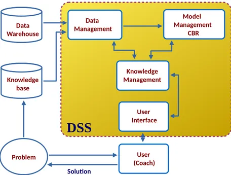
Figure 1.1 Flow diagram of the DSS components...5

Figure 1.2 Intelligence stage of the DSS framework design... 5

Figure 1.3 Design stage of the DSS framework...6

Figure 1.4 Production-rules system architecture...8

Figure 1.5 DSS conceptual framework...13

Figure 1.6 Standard statistical information of a final match competition...14

Figure 1.7 Standard stats information of the team Argentina describing the zone of attack...15

Figure 1.8. Standard stats information of the team Germany describing the zone of attack... 16

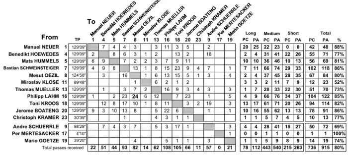
Figure 1.9 Passing distribution of the two teams...17

Figure 1.10 Standard normal distribution of matches rating...19

Figure 1.11 Distribution of classes: Home wins, Away wins and Draws...21

Figure 1.12 Anatomy of a multipolar neuron...23

Figure 1.13 An artificial neural network is an interconnected group of nodes...24

Figure 1.14 Training phase of ANN...25

Figure 1.15 Competitive learning of ANN...25

Figure 1.16 Reinforcement learning of ANN...25

Figure 1.17 The Perceptron (Rosenblatt '58)...26

Figure 1.18 Searching space of a learning rule...31

Figure 1.19 A sequential covering algorithm...31

Figure 2.1 Pitch divisions in three thirds parallel to the goal lines...34

Figure 2.2 A diagrammatic representation of the proposed system framework...35

Figure 2.3 Data input of the multilayer perceptron obtained from soccerdb...36

Figure 2.4 Example of multilayer perceptron in weka...37

Figure 2.5 Drill design of Pulling along defenders into the decision support system...38

Figure 2.6 Drill design of Central penetrating run into the decision support system...38

Figure 2.7 Drill design of Fullback crossing into the decision support system...39

Figure 2.8 Drill design of Arranging players with a deep attack into the system...39

Figure 2.9 Drill of Passing out wide to the fullback in the decision support system...40

Figure 2.10 Drill of Play for fullbacks in the decision support system...40

Figure 2.11 Drill of Play for wingers into the system...41

Figure 2.12 Drill of Passing and receiving, angles of support into the system...41

Figure 2.13 Drill of Play with fullbacks into the system...42

Figure 2.14 Drill of Possession into the system...43

Figure 2.15 Drill of Passing in two boxes into the system...44

Figure 2.16 Drill of Three servers, 1 shooting player into the system...44

Figure 2.17 Drill of One-touch finishing...45

Figure 2.18 Database model in mysql called soccerdb...46

Figure 2.19 Implementation of SCDSS in Eclipse platform...47

Figure 2.20 Java object code fragment inside the system...47

Figure 3.1 Prediction tabbedpane of the winner or maybe a draw as a match result...49

Figure 3.2 Stats tabbedpane for training direction work and feature stats analysis...50

Figure 3.3 Model tabbedpane for teams feature stats analysis comparison...50

(11)

Index of Tables

Table 1.1 Description and measurement of attacking and defensive performance indicators ...18 Table 1.2 Goal match ratings with percentages...20 Table 1.3 Fair odds expectancies...22

(12)

Introduction

The savage essence and nature of sports means those who work on it hunt for the wins. The sport enterprise is undergoing a gigantic digital transformation focused on imaging, real time and data analysis employed in the competitions. Conventional process methods in sports management such as fitness and health establishments, training, growth and match or game realisation are all being revolutionized by the sport digitization. In team sports it is well known that is needful an enough and simple digital methodology to organize and construct a feasible strategy. Digitization in sports is perpetually evolving and requires pervasive challenges. The sports and athletics digitization success is based on what is being done with collection of more data. Competitive advantages go to those who produce powerful operations using the data and acting on it in real time. The potential impact of these sport features in sport team operations is powerful. Data does not ride all decisions, but it empowers knowledgeable decisions.

In these world circumstances, our vision with this system was born from a dream helping soccer sport management systems embrace and improve its contest success. Our perspective problem is how a decision support system for soccer coaches helps them to take enhancement decisions better. To face this problem we have created a soccer coach decision support system. This system is organised in two joined components; the first simulates the prediction of the soccer match winner through a data driven neural network. This component output activates the second to operate the logic rules learning and provides the stats, analysis, decision making and additionally plans improvements like drills and training procedures. This helps on the preparation towards upcoming matches as well as being aligned with their style and playing concepts.

Future scalabilities and developments, will analyse timely the mental and moral features of the teams because their importance is seen when teams or athlete’s behavior change and they display unexpected performance with astonishment match results.

(13)

Chapter 1 Overview of decision support systems

and soccer management methods

1.1 Decision Support Systems, Categorization and Development

When it comes to good decision making [1], relying too heavily on automatic decisions stemming from perception or depending too much on conventions when information is bombarded on to us from all sides can be dangerous. Sometimes, we fail to either notice or seek out crucial information that supports decision making. This may be because of our biasness or shortage of time, funds and other resources.

In many situations, we are unable to apply fundamentals of economics, statistics and operations research to make lucid choices. This is where a decision support system comes into picture. It is a computer-based system that helps us make planning, manufacturing, operations and management decisions, based on information available. But these systems are not the decision makers. They just aid in decision making, by offering insights that we may be missing and in providing exact calculations but the ultimate decision maker are only us.

1.1.1 Decision Support System (DSS)

A decision support system:

 is a computer-based application or program

 that compiles, combines and analyzes raw data, documents, fundamentals of social science, applied science, mathematics and managerial science, and personal knowledge of decision makers

(14)

 to identify problems and determine their solutions  in order to facilitate optimal decision making.

A decision support system helps overcome the barriers to a good decision making, including:  lack of experience

 biasness

 shortage of time  wrong calculations

 not considering alternatives

The Decision Support Systems can be divided into following categories:

1.1.1.1 Model-driven DSS

A model-driven DSS is based on simple quantitative models. It uses limited data and emphasized manipulation of financial models. A model-driven DSS is used in production planning, scheduling and management. It provides the most elementary functionality to manufacturing concerns.

1.1.1.2 Data-driven DSS

Data-driven DSS emphasizes the access and manipulation of data tailored to specific tasks using general tools. While it also provides elementary functionality to businesses, it relies heavily on time-series data. It is able to support decision making in a range of situations.

1.1.1.3 Communication-driven DSS

As the name suggests, communication-driven DSS uses communication and network technologies to facilitate decision making. The major difference between this and the previous classes of DSS is that it supports collaboration and communication. It made use of a variety of tools including computer-based bulletin boards, audio and video conferencing.

1.1.1.4 Document-driven DSS

A document-driven DSS uses large document databases that stores documents, images, sounds, videos and hypertext docs. It has a primary search engine tool associated for searching the data when required. The information stored can be facts and figures, historical data, minutes of meetings, catalogs, business correspondences, product specifications, etc.

1.1.1.5 Knowledge-driven DSS

Knowledge-based DSS are human-computer systems that come with a problem-solving expertise. These combine artificial intelligence with human cognitive capacities and can suggest actions to users. The notable point is that these systems have expertise in a particular domain.

(15)

1.1.1.6 Web-based DSS

Web-based DSS is considered most sophisticated decision support system that extends its capabilities by making use of worldwide web and internet. The evolution continues with advancement in internet technology.

DSS applications are not single information resources, such as a database or a program that graphically represents sales figures, but the combination of integrated resources working together. These can support decision making in situations where precision is of importance. Additionally, they provide access to relevant knowledge by integrating various forms and sources of information, aiding human cognitive deficiencies. While DSS employs artificial intelligence to address problems, the end decision remains with the user.

1.1.2 Categorization/Classification of DSS

Let us now look at the categorization on the basis of nature of operations:

1.1.2.1 File Drawer System

As the name suggests, a file drawer decision support system provides information useful for making a specific decision. It works like a file drawer where different types of information are stored under different names or categories.

1.1.2.2 Data Analysis Systems

These decision support systems are based on a formula; and therefore, are used to make comparative analysis. These make use of simple data processing tools, such as inventory analysis.

1.1.2.3 Information Analysis System

This kind of decision support system analyzes different sets of data to generate informational reports that can be used to assess a situation for decision making.

1.1.2.4 Accounting and Financial Support System

This type of support system is based on to keep track of cash and inventory.

1.1.2.5 Representation or Solver Model

This type of system performs or represents decision making in a particular domain or for a specific problem. It calculates and compares the outcomes of different decision paths. The decision maker can conduct a ‘what if’ analysis and make an informed decision basis on the outcomes generated.

1.1.2.6 Optimization Model

This DSS is based on simulated models, majorly providing guidelines for operations management. The focus is on providing optimal solutions on job scheduling, product mix and material mix decisions.

(16)

1.1.2.7 Suggestion System

This type of support system suggests optimal decision for a particular situation by assisting in collecting and structuring data.

1.1.2.8 Categorization of DSS on the Basis of Inputs

 Text Oriented DSS  Database Oriented  Spreadsheet Oriented  Rule Oriented

 Solver (specific situation) Oriented

 Compound/Hybrid: This support system combines two or more structures from above to offer multiple functionalities.

1.1.2.9 Categorization of DSS on the Basis of Support Offered

 Personal DSS  Group DSS

 Organizational DSS

1.1.2.10 Categorization of DSS on the Basis of Type and Frequency of Decision Making a. Institutional DSS

An institutional decision support system supports recurring decisions on an ongoing basis. Basically, this is for programmed decisions, which are made on daily basis. For example, establishing routine for handling technical problems, taking disciplinary actions, unit manufacturing, a mechanic process of troubleshooting, etc.

b. Ad-hoc DSS

An ad-hoc decision support system supports one kind of decision in an unanticipated situation. The decision made is unique to a problem. This type of system is used to support non-programmed decisions as the information available is incomplete.

1.1.3 Components of a Decision Support System

Like any other software system, DSS also has components and phases of development. No matter what kind of decision support system we are looking to develop, we must plan around these four components:

 Input: What kind of input does it require to carry out the analysis? As mentioned earlier, it can be rule, problem, spreadsheet, text or database oriented.

(17)

 User Knowledge/Expertise: Whether inputs will require manual analysis by the user or not.  Output: Should the outcomes be comparative or generic?

 Decisions: Whether it should be a suggestion support system? Or we just want it to analyze the data and outcome of different actions?

1.1.4 Designing and Building a Decision Support System

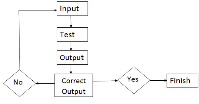
Developing a DSS is a complex process and thus, takes longer. It goes repetitively through three stages: inputs, activities and outputs during each phase of system development lifecycle. We provide an input, carry out the desired activity and measure the output. Moving us further, if it produces the right output or else we come back to the input phase and make adjustments.

Figure 1.1 Flow diagram of the DSS components.

A DSS framework design and development goes through these stages:

1.1.4.1 Intelligence

At this stage, the objective is to search for problems/situations/conditions that call for decision.

(18)

The user, as an expert, is expected to identify and define the problem context for which support is required. He must define the objectives and available resources, so that the outcomes generated meet his expectations.

1.1.4.2. Design

This stage deals in analyzing all possible actions, along with the determination of system design and system construction.

Figure 1.3 Design stage of the DSS framework.

System design includes determination of components, platform, function libraries and special languages while system structure is about deciding the prototype approach. This stage also includes identifying hardware requirements. The development starts here.

1.1.4.3 Choice

Once we shortlist and analyze all possible courses of actions in design phase, now is the time to choose the best from among them, depending upon our business objectives and results generate.

1.1.4.4 Implementation

This is the final stage where testing, evaluation, adjustments and deployment take place. However, this is the final product but this can be tweaked, refined and upgraded basis your activities and requirements.

When developing a custom DSS, these are important factors that must be kept in mind:  Data management functions

 Available hardware platforms  User interface

 Compatibility with other applications  Cost

(19)

1.1.5 Building Knowledge-Driven Decision Support System and Mining Data

Before the development of knowledge-driven DSS, people with high intellect had to perform knowledge-intensive tasks. An expert in a particular area would know how to approach a problem and go about it. Similarly, knowledge-based DSS asks relevant questions, offers suggestions and gives advice to solve a problem. The only difference is that it is automated and speeds up the whole process.

1.1.5.1 Knowledge-Driven DSS

A knowledge-driven DSS:

 is a computer-based reasoning system

 that provides information, comprehension and suggestions to users  to support them in decision-making.

It is an integration of computerized business intelligence tools and technologies customized to the needs and requirements of an organization. So, the focus is on:

 Identifying specific knowledge sharing and distribution needs of a company  Setting objectives that need to be attained with a knowledge-driven DSS  The selection of appropriate tools and technologies

 Understanding the nature of work and decision-making performed by its potential users  Selecting data mining techniques

1.1.5.2 Key Terms and Concepts

A computer-based reasoning system is similar to any other type of decision support system when it comes to their architecture. But it turns into a knowledge-drive decision support system when artificial intelligence technologies, management expert systems, data mining capabilities and other communication mechanisms are integrated.

Let us learn about few important terms and concepts used alongside knowledge-driven decision support system. This will help gain an in-depth understanding of such support systems.

a. Expertise

A knowledge-driven DSS comes with a specific problem-solving expertise. This expertise is based upon three components:

 Knowledge in a particular domain and associated symptoms and signs.  Understanding of the relationships between varied symptoms of a problems.  Skills, ways or methods of solving the problem.

(20)

b. Expert System

A computer system that imitates the decision making capability of a human expert is called an expert system or an artificial intelligence system. It is designed to solve problems by:

 Using if-then rules

 Reasoning about knowledge

 Drawing inferences from facts and rules

b.1 Production-rule systems b.1.1 Definition

Programs that implement research methods for problems represented as state space [2]. They consist of:

– a set of rules,

– a 'working memory', which contains the current states reached

– a control strategy to select the rules to be applied at the states of the 'working memory' (matching, verification of preconditions and test on goal state if achieved).

General Architecture:

Figure 1.4 Production-rules system architecture.

b.2 Two modalities of "reasoning" b.2.1 Forward or data-driven

– The working memory in its initial configuration contains the initial knowledge about the problem, those are the known facts.

(21)

– The applicable production rules are those whose antecedent can match with the working memory (F-rules).

– Each time a rule is selected and performed, new demonstrated facts are inserted in the working memory.

– The procedure ends with success when in the working memory the goal to be demonstrated is also inserted (termination condition).

b.2.2 Backward or goal-driven

– The initial working memory contains the goal (or goals) of the problem.

– The applicable production rules are those whose consequent can match with the working memory (B-rules).

– Each time a rule is selected and executed, new subgoals to be demonstrated are inserted into the working memory.

– The process ends with success when in the working memory are inserted known facts (termination condition).

c. Knowledge Discovery and Data Mining

These are interrelated terms used for the process of extracting valuable knowledge and discovering patterns, in order to transform the knowledge into easily comprehendible structure for further use. Data mining is a buzzword but a misnomer. This is because data mining is a process of collection, storing and analysis of data and not finding patterns. Knowledge discovery goes through a series of steps:  Selection  Pre-processing  Transformation  Data mining  Interpretation d. Development Environment

It is the environment in which a decision support system is developed. It typically includes software for creating a DSS and knowledge base. The development environment may vary in size, depending upon production/development needs.

e. Domain Expert

A domain expert is a subject matter expert who has expertise/authority in a particular domain. A domain expert is an integral part of the team working on developing a decision support system.

(22)

f. Knowledge Engineer

A technical expert who integrates knowledge into a computer system when developing a decision support system, in order to solve complex problems that require human expertise.

g. Knowledge Acquisition

It is extraction/mining of knowledge from various sources, such as experts, databases and external programs.

h. Knowledge Base

It is the collection and storage of structured (facts, rules, regulations, characteristics, functions, procedures and relationships) and unstructured information that will be used by a DSS in decision making.

i. Interface Engine

It is a software system to simplify the conception and development of application interfaces between application systems. Typically, it is a middleware application to transform, route and translate messages between various communication points.

j. Heuristic

It is an approach to discovery and problem solving by employing practical methods. These methods may not be optimal but can help achieve immediate goals.

These technical jargons are important in this field of use, in order to gain a deeper understanding of knowledge-driven DSS.

1.1.5.3 Characteristics of Knowledge-Driven Decision Support Systems

A knowledge-driven DSS is different from conventional systems in the way knowledge is extracted, processed and presented. The former attempts to emulate human reasoning while the latter responses to an even in a predefined manner. The main characteristics of knowledge-driven decision support systems are:

 These systems aid managers in solving complex problems.

 These systems allow users to interact with them during the process of decision making.  The recommendations made by these systems are based on human knowledge.

 These systems use knowledge base that is engineered keeping in mind the nature of problems they will solve.

 These systems aid in performing limited tasks.

(23)

1.1.5.4 Managing Knowledge-Driven Decision Support System Projects

Knowledge-driven decision support systems are expert systems that are developed when decision-making cannot be supported using traditional methods. A knowledge-driven DSS project goes through various stages and can be difficult to manage. It is important to be committed to monitor the development of a knowledge-driven DSS.

1.1.5.4.1 Development Stages

 Domain identification (choosing a subject matter)

 Conceptualization (idea formation, feasibility testing and commencement)  Formalization (beginning with development officially)

 Implementation (completion and execution)  Testing (fixing errors and modifications)

It is important to monitor project development throughout very closely. It is a collective effort of knowledge engineers, domain experts, DSS analysts, users and programmers. And a project manager keeps track of the scope, time, quality and budget, to ensure optimum allocation of resources and creation of a quality product. A project manager is a person responsible for accomplishing the pre-decided objectives of a project.

1.1.5.5 Tools and Techniques

There are a large number of tools and techniques used to extract/mine data. Which technique is to be used depends on the type of data to be extracted.

a. Case-based Reasoning

Case-based reasoning (CBR) tools are used to determine the distance between or relationship among various components. A problem solved using this tool goes through five stages:

 Presentation – the problem is described and entered into the system.  Retrieval – the system matches it with the cases stored in the system.

 Adaptation – the system matches the retrieved closest-matching case and the problem to generate a solution.

 Validation - the solution then goes through a validity test and is justified if the user gives a positive feedback.

 Update – the valid solution is accepted and added to the case base in the system.

b. Fuzzy Query and Analysis

Fuzzy query and analysis is a data mining tool follows the mathematical concept for ‘fuzzy logics – the logic of uncertainty’ to determine results that are close to a particular criterion. Users can then pick one, depending upon his or her understanding.

(24)

c. Data Visualization

As the same suggests, this helps analysts visualize complex relationships in multi-dimensional data. The benefit is that this tool graphically represents relationships among components from different perspectives. Statistical tools, such as regression, classification or cluster analysis are a part of this tool.

d. Genetic Algorithms

Similar to linear programming models, genetic algorithms conduct random experiments by selecting the genes (variables whose values are to be identified) and their values at random to find the fitness function. The software will also combines and mutates genes to find optimized value.

e. Neural Networks

Neural network tools are used to predict future information by learning patterns and then applying them to predict future relationships. Neural networks attempt to learn patterns from data directly by repeatedly examining the data to identify relationships and build a model. They build models by trial and error. The network guesses a value that it compares to the actual number. If the guess is wrong, the model is adjusted. This process involves three iterative steps: predict, compare, and adjust. Neural networks are commonly used in a DSS to classify data and, as noted, to make predictions. [3]

1.1.5.6 Evaluating Development Packages

Whenever it is decided to develop or purchase a knowledge-driven decision support system software application, it is important to consider following criteria:

a. Development Features: Input rules, customizability, capabilities and maintenance.

b. Scalability: Ease of integration with other existing hardware and software, web technologies,

operating systems.

c. Ease of Use and Installation: The ease with which end user will be able to work on it. d. Security: Safety of data and company information.

e. Cost: Cost of technology, cost of development, maintenance cost.

Knowledge-driven decision support systems help businesses solve problems and make decisions. However, a caution should be used when employing it. It does not outsmart human intellect; rather it aids decision making.

(25)

Figure 1.5 DSS conceptual framework.

1.2 Soccer management methods

Soccer coach management methods describe the decision process of a coach for analysing and planning the operations approach used to qualify a team to the competitions. There are three different levels of reviewing this goal: statistical data analysis, prediction method, and afterwards operation planning.

Conventional sport methods labor the most times in drilling plans analysis with habitual stats information of contender teams. This vision generally means a unvarying prospective knowledge and this coach working mostly times gets hard losses.

1.2.1 Stats analysis

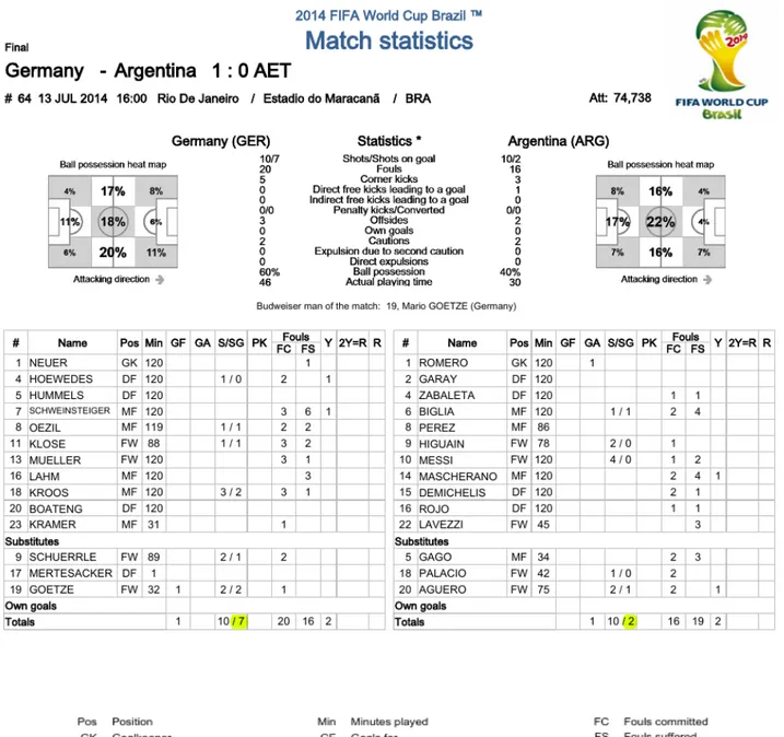
FIFA World Cup stats gives a complete analysis for each match played by the two contender teams in competition. Nextly in Figure 1.6 we show a statistical match result of the 2014 championship final contended by Germany and Argentina.

According to previous research and literature relating to soccer prediction [5], we get tactic, planning and attacking as performance indicators in competition matches. Therefore we consider these concepts to model the stats reports, which means: Shots on target, Possession of the ball and Score (Figure 1.6 [6]), Possession of the ball in the attacking third of the pitch, Forwards passes and Passes from defensive to attacking third (Figures 1.7 [7], 1.8 [8]). Passing accuracy is taken from Passing distribution showed on Figure 1.9 [9]. Some description and measurement methods are presented in Table 1.1 Data Management Model Management CBR Soluton User Interface Knowledge Management User (Coach) Problem Data Warehouse Knowledge base

DSS

(26)

Figure 1.6 Shows the standard statistical information of a final match competition1_.

(27)

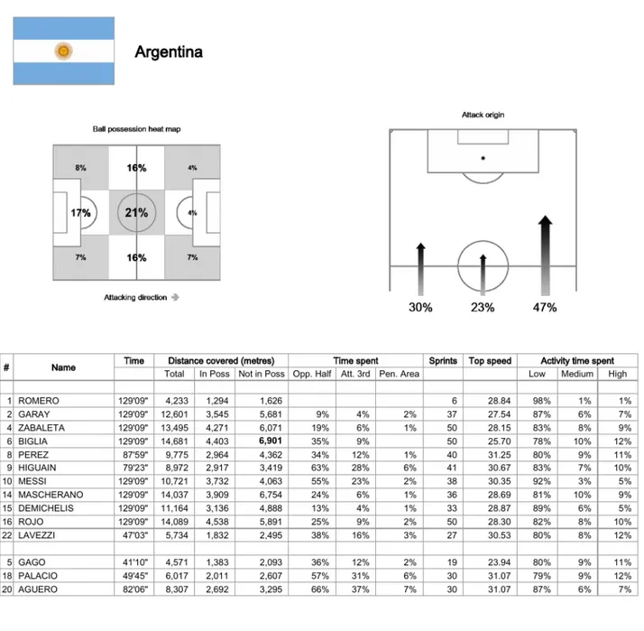
Figure 1.7 Standard statistical information of the team Argentina describing the zone of attack2_.

2 http://resources.fifa.com/mm/document/tournament/competition/02/40/51/10/64_0713_ger-arg_arg_teamstatistics.pdf

(28)

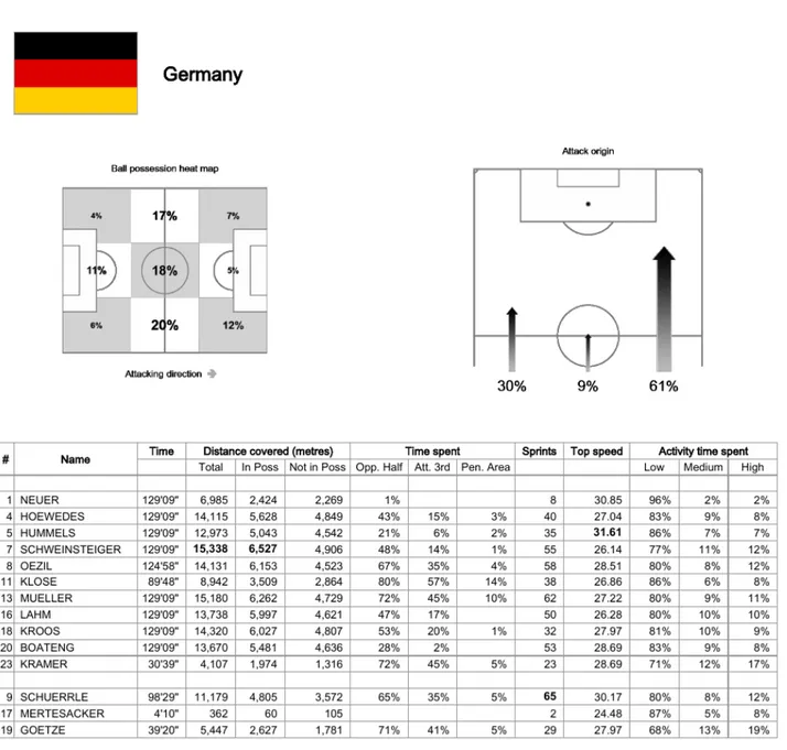
Figure 1.8. Standard statistical information of the team Germany describing the zone of attack3_.

3 http://resources.fifa.com/mm/document/tournament/competition/02/40/50/84/64_0713_ger-arg_ger_teamstatistics.pdf

(29)

(30)

Attacking performance indicators Description Measurement 1. Possession of the ball

Percentage of time that the team has possession of the ball in the match.

Possession of the ball for the team was collected separately for each half of the match as it is provided by the Amisco system [10]. The average from the possession of the two halves for each team was calculated.

These performance indicators were calculated by taking the overall time that the team had the possession of the ball and the time that the team had the possession of the ball in the area corresponding to the performance indicator. Hence the percentage (normalised data) was calculated from these data provided by the Amiscosystem.

2. Possession of the ball in the attacking third of the pitch.

Percentage of time that the team have the possession of the ball in the attacking third of the pitch (next to the opposite goal) from all the time that the team have the possession of the ball.

3. Forwards passes Percentage of passes from the overall number of passes made by the team that are made forwards (towards the opposite goal).

The Amisco system provided the direction of the movements of the ball by looking at the point where the pass started and the point where the pass was received. Data was normalised by calculating the percentage of these passes according to the total number of passes made by the team.

4. Passes from defensive third to attacking third

Percentage of passes from the overall number of passes made by the team that are made directly from the defensive third (next to the own goal) to the attacking third of the pitch (next to the opposite goal).

These performance indicators were measured by calculating the percentage of these kinds of passes from the overall amount of passes made by the team in the match.

Table 1.1 Description and measurement of attacking and defensive performance indicators [11]. 1.3 Methods of prediction

Rating methods is commonly used in mostly cases. It is showed below.

1.3.1 Rating Systems for Fixed Odds Football Match Prediction

It is defined [12], by analysing and comparing one or more aspects of past performance for each of the teams, whilst more complex ratings might be based on elaborate match statistics including shots on goal, corners, and even possession if such data are available. A simple way looks at the number of goals scored and conceded by the two teams for a specified number of matches preceding the contest under examination. A match rating must in some way be translated into a probability distribution for the three possible results in a football match: home win, the draw and away win.

1.3.1.1 A Goals Superiority Rating System

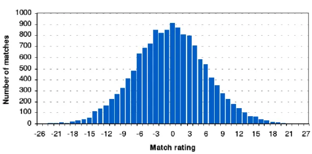
The assumption for a goals superiority rating system, then, is that teams who score more goals and concede fewer over the course of a number of matches are more likely to win their next game. To see how a goal superiority match rating is calculated, consider the following example for a game played between Tottenham and Leeds at White Hart Lane. In their last 6 games, Tottenham have scored 6 goals and conceded 9. Meanwhile, Leeds have scored 8 times and conceded 11 goals. Tottenham's goal superiority rating for the last 6 games is -3; for Leeds it is also -3. The match

(31)

rating is simply given by the home side's rating minus the away side's rating, and for this match is therefore 0. Using results data for the English Premiership and Divisions 1, 2, and 3 for seasons 1993/94 to 2000/01, goal supremacy ratings for the last 6 matches played by every team have been calculated. Of the 16,272 matches played during these 8 years, 14,002 of them were eligible for a rating calculation, with the matches played in the earlier weeks of each season obviously unsuitable for recent form analysis. The number of matches with each rating and percentages are shown in the figures below.

Figure 1.10 Standard normal distribution of matches rating.

1.3.1.2 Defining the Fair Odds

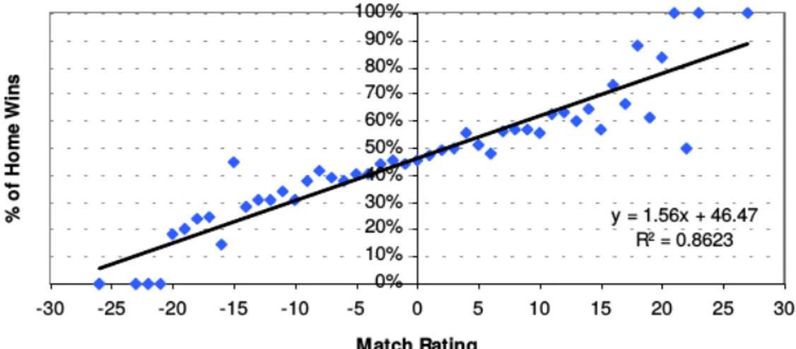
The first task is to consider each result independently, and identify the "best-fit" relationship with the match ratings. The easiest way to determine this best-fit relationship is to draw the match ratings and result probabilities as three scatter plots, one for each result, as shown on Figure 1.11. This can be done simply using any spreadsheet. For each scatter plot, the best fit line (with its equation) has been superimposed on the data points, representing what would statistically be considered to be the best relationship between match rating and result probability.

The value of R2_{shown for each of the three equations is simply a statistical measure of how closely}

the real data match the best-fit lines. A perfect relationship, denoted by R2_{= 1, would mean that the}

best-fit line and equation describe perfectly the real data. Consequently, a fairly good relationship exists between the match rating and home win probability, where as much as 86% of the variation in the real data is explained by its best-fit equation. For away wins and particularly draws the relationship is weaker. With each equation we can easily determine the expected probability of a home win, draw and away win for any match where we have calculated the goal supremacy rating. For the Tottenham-Leeds game, where the match rating was 0, the probability of a home win, for example, can be determined using: y = 1.56x + 46.47

(32)

(33)

(34)

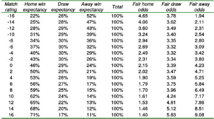
With an estimation of the probability or expectancy for a home win we can easily define the fair odds for a home win, using:

100 divided by probability of home win Fair odds for some other match ratings are show tabulated below.

Table 1.3 Fair odds expectancies.

This method could be used for analogous prediction analysis and therefore it can be performed for national soccer team tournament predictions.

1.3.2 Artificial neural networks learning 1.3.2.1 Biological neural network

In neuroscience [13], a biological neural network is a series of interconnected neurons whose activation defines a recognizable linear pathway. The interface through which neurons interact with their neighbors usually consists of several axon terminals connected via synapses to dendrites on other neurons. If the sum of the input signals into one neuron surpasses a certain threshold, the neuron sends an action potential at the axon hillock and transmits this electrical signal along the axon.

(35)

Figure 1.12 Anatomy of a multipolar neuron.

The first rule of neuronal learning was described by Hebb in 1949, Hebbian learning. Thus, Hebbian pairing of pre-synaptic and post-synaptic activity can substantially alter the dynamic characteristics of the synaptic connection and therefore facilitate or inhibit signal transmission. The neuroscientists Warren Sturgis McCulloch and Walter Pitts published the first works on the processing of neural networks. They showed theoretically that networks of artificial neurons could implement logical, arithmetic, and symbolic functions. Simplified models of biological neurons were set up, now usually called perceptrons or artificial neurons.

1.3.2.2 Artificial neural network

Artificial neural networks (ANNs) or connectionist systems are computing systems inspired by the biological neural networks that constitute animal brains [14]. Such systems learn (progressively improve their ability) to do tasks by considering examples, generally without task-specific programming. For example, in image recognition, they might learn to identify images that contain cats by analyzing example images that have been manually labeled as "cat" or "no cat" and using the analytic results to identify cats in other images. They do this without any a priori knowledge about cats, e.g., that they have fur, tails, whiskers and cat-like faces. Instead, they evolve their own set of relevant characteristics from the learning material that they process. They have found most use in applications difficult to express with a traditional computer algorithm using rule-based programming.

An ANN is based on a collection of connected units or nodes called artificial neurons (a simplified version of biological neurons in an animal brain). Each connection (a simplified version of a synapse) between artificial neurons can transmit a signal from one to another. The artificial neuron that receives the signal can process it and then signal artificial neurons connected to it.

In common ANN implementations, the signal at a connection between artificial neurons is a real number, and the output of each artificial neuron is calculated by a non-linear function of the sum of

(36)

its inputs. Artificial neurons and connections typically have a weight that adjusts as learning proceeds. The weight increases or decreases the strength of the signal at a connection. Artificial neurons may have a threshold such that only if the aggregate signal crosses that threshold is the signal sent. Typically, artificial neurons are organized in layers. Different layers may perform different kinds of transformations on their inputs. Signals travel from the first (input), to the last (output) layer, possibly after traversing the layers multiple times.

Figure 1.13 An artificial neural network, akin to the vast network of neurons in a brain. Each circular node represents an artificial neuron and an arrow represents a connection from the output of one artificial neuron to the input of another.

The original goal of the ANN approach was to solve problems in the same way that a human brain would. However, over time, attention focused on matching specific tasks, leading to deviations from biology. ANNs have been used on a variety of tasks, including computer vision, speech recognition, machine translation, social network filtering, playing board and video games and medical diagnosis.

1.3.2.2.1 Learning paradigms

The three major learning paradigms applied to ANNs correspond to a particular learning task. These are supervised learning, unsupervised learning (competitive learning) and reinforcement learning.

a. Supervised learning

It is the most widely used where the network learns to recognize a set of desired input configurations [15]. It learns to associate a set of given pairs (Xk,Ydk) (Figure 1.14). The network

operates in two distinct phases:

• Learning phase – it stores the desired information via examples. • Evolution phase – it retrieves the stored information.

(37)

Supervised learning is the machine learning task of learning a function that maps an input to an output based on example input-output pairs [16]. It infers a function from labeled training data consisting of a set of training examples. In supervised learning, each example is a pair consisting of an input object (typically a vector) and a desired output value (also called the supervisory signal). A supervised learning algorithm analyzes the training data and produces an inferred function, which can be used for mapping new examples. An optimal scenario will allow for the algorithm to correctly determine the class labels for unseen instances.

Figure 1.14 Training phase of ANN.

b. Competitive learning

• Neurons compete for specializing in the recognition of a particular stimulus. Similar stimulus end up in the same class. In the end, each neuron is activated by a given stimulus (isomorphism between stimuli and output neurons).

Figure 1.15 Competitive learning of ANN.

c. Reinforcement learning

• Reinforcement learning simulates the learning mechanism in animals based on reward and punishment: used for control systems applications.

(38)

1.3.2.2.2 Perceptron

In machine learning [17], the perceptron is an algorithm for supervised learning of binary classifiers (functions that can decide whether an input, represented by a vector of numbers, belongs to some specific class or not). It is a type of linear classifier, i.e. a classification algorithm that makes its predictions based on a linear predictor function combining a set of weights with the feature vector. The algorithm allows for online learning, in that it processes elements in the training set one at a time.

The perceptron algorithm dates back to the late 1950s. Its first implementation, in custom hardware, was one of the first artificial neural networks to be produced. Figure 1.17 represent this abstraction.

Figure 1.17 The Perceptron (Rosenblatt '58)

1.3.2.2.3 Deep learning

Deep learning (also known as deep structured learning or hierarchical learning) is part of a broader family of machine learning methods based on learning data representations, as opposed to task-specific algorithms. Learning can be supervised, semi-supervised or unsupervised. [18]

Deep learning models are loosely related to information processing and communication patterns in a biological nervous system, such as neural coding that attempts to define a relationship between various stimulus and associated neuronal responses in the brain.

Deep learning architectures such as deep neural networks, deep belief networks and recurrent neural networks have been applied to fields including computer vision, speech recognition, natural language processing, audio recognition, social network filtering, machine translation, bioinformatics and drug design, where they have produced results comparable to and in some cases superior to human experts.

(39)

 use a cascade of multiple layers of nonlinear processing units for feature extraction and transformation. Each successive layer uses the output from the previous layer as input.  learn in supervised (e.g., classification) and/or unsupervised (e.g., pattern analysis) manners.  learn multiple levels of representations that correspond to different levels of abstraction; the

levels form a hierarchy of concepts.

a. Concepts

The assumption underlying distributed representations is that observed data are generated by the interactions of layered factors.

Deep learning adds the assumption that these layers of factors correspond to levels of abstraction or composition. Varying numbers of layers and layer sizes can provide different degrees of abstraction. Deep learning exploits this idea of hierarchical explanatory factors where higher level, more abstract concepts are learned from the lower level ones.

Deep learning architectures are often constructed with a greedy layer-by-layer method. Deep learning helps to disentangle these abstractions and pick out which features improve performance. For supervised learning tasks, deep learning methods obviate feature engineering, by translating the data into compact intermediate representations akin to principal components, and derive layered structures that remove redundancy in representation.

Deep learning algorithms can be applied to unsupervised learning tasks. This is an important benefit because unlabeled data are more abundant than labeled data. Examples of deep structures that can be trained in an unsupervised manner are neural history compressors and deep belief networks.

b. Interpretations

Deep neural networks are generally interpreted in terms of the universal approximation theorem [19] or probabilistic inference [20].

The universal approximation theorem concerns the capacity of feed forward neural networks with a single hidden layer of finite size to approximate continuous functions. In 1989, the first proof was published by Cybenko for sigmoid activation functions and was generalised to feed-forward multi-layer architectures in 1991 by Hornik.

Universal approximation properties and depth: Feed forward network with at least one hidden layer provide a universal approximation framework [21].

The probabilistic interpretation derives from the field of machine learning. It features inference, as well as the optimization concepts of training and testing, related to fitting and generalization, respectively. More specifically, the probabilistic interpretation considers the activation nonlinearity as a cumulative distribution function. The probabilistic interpretation led to the introduction of dropout as regularizer in neural networks. The probabilistic interpretation was introduced by

(40)

researchers including Hopfield, Widrow and Narendra and popularized in surveys such as the one by Bishop.

c. Deep neural networks

A deep neural network (DNN) is an ANN with multiple hidden layers between the input and output layers [22]. DNNs can model complex non-linear relationships. DNN architectures generate compositional models where the object is expressed as a layered composition of primitives. The extra layers enable composition of features from lower layers, potentially modeling complex data with fewer units than a similarly performing shallow network.

Deep architectures include many variants of a few basic approaches. Each architecture has found success in specific domains. It is not always possible to compare the performance of multiple architectures, unless they have been evaluated on the same data sets.

DNNs are typically feedforward networks in which data flows from the input layer to the output layer without looping back. Recurrent neural networks (RNNs), in which data can flow in any direction, are used for applications such as language modeling. Long short-term memory is particularly effective for this use.

Convolutional deep neural networks (CNNs) are used in computer vision. CNNs also have been applied to acoustic modeling for automatic speech recognition (ASR).

d. Multilayer perceptron

A multilayer perceptron (MLP) is a class of feedforward artificial neural network [23]. An MLP consists of at least three layers of nodes. Except for the input nodes, each node is a neuron that uses a nonlinear activation function. MLP utilizes a supervised learning technique called backpropagation for training. Its multiple layers and non-linear activation distinguish MLP from a linear perceptron. It can distinguish data that is not linearly separable.

d.1 Activation function

If a multilayer perceptron has a linear activation function in all neurons, that is, a linear function that maps the weighted inputs to the output of each neuron, then linear algebra shows that any number of layers can be reduced to a two-layer input-output model. In MLPs some neurons use a nonlinear activation function that was developed to model the frequency of action potentials, or firing, of biological neurons.

The two common activation functions are both sigmoids, and are described by

y ( v_i)=tanh (v_i) and y ( v_i)=(1+e−vi)−1

The first is a hyperbolic tangent that ranges from -1 to 1, while the other is the logistic function, which is similar in shape but ranges from 0 to 1. Here yi is the output of the ith node (neuron) and

(41)

d.2 Layers

The MLP consists of three or more layers (an input and an output layer with one or more hidden layers) of nonlinearly-activating nodes making it a deep neural network. Since MLPs are fully connected, each node in one layer connects with a certain weight wij to every node in the following

layer.

d.3 Learning

Learning occurs in the perceptron by changing connection weights after each piece of data is processed, based on the amount of error in the output compared to the expected result. This is an example of supervised learning, and is carried out through backpropagation, a generalization of the least mean squares algorithm in the linear perceptron.

We represent the error in output node j in the nth data point (training example) by

e_j(n)=d_j(n)−y_j(n)

where d is the target value and y is the value produced by the perceptron. The node weights are adjusted based on corrections that minimize the error in the entire output, given by

ε(n)=1 2

∑

_j ej

2 (n)

Using gradient descent, the change in each weight is

Δw_ji(n)=−η ∂ ε(n) ∂v_j(n)yi(n)

where yi is the output of the previous neuron and η is the learning rate, which is selected to ensure

that the weights quickly converge to a response, without oscillations.

The derivative to be calculated depends on the induced local field vj , which itself varies. It is easy

to prove that for an output node this derivative can be simplified to

− ∂ ε(n)

∂v_j(n)

=e_j(n)ϕ'(v_j(n))

where ϕ’ is the derivative of the activation function described above, which itself does not vary. The analysis is more difficult for the change in weights to a hidden node, but it can be shown that the relevant derivative is − ∂ ε(n) ∂v_j(n) =ϕ'(v_j(n))

∑

k − ∂ ε(n) ∂v_k(n)wkj (n)

This depends on the change in weights of the kth nodes, which represent the output layer. So to change the hidden layer weights, the output layer weights change according to the derivative of the activation function, and so this algorithm represents a backpropagation of the activation function.

(42)

1.3.3 Logic learning machine (LLM)

Machine learning method based on the generation of intelligible rules [24]. LLM is an efficient implementation of the Switching Neural Network (SNN) paradigm, developed by Marco Muselli, Senior Researcher at the Italian National Research Council CNR-IEIIT in Genoa. Logic Learning Machine is implemented in the Rulex suite.

LLM has been employed in different fields, including orthopaedic patient classification, DNA microarray analysis and Clinical Decision Support System.

1.3.3.1 General

Like other machine learning methods, LLM uses data to build a model able to perform a good forecast about future behaviors. LLM starts from a table including a target variable (output) and some inputs and generates a set of rules that return the output value corresponding to a given configuration of inputs. A rule is written in the form:

where consequence contains the output value whereas premise includes one or more conditions on the inputs. According to the input type, conditions can have different forms:

 for categorical variables the input value must be in a given subset:

 for ordered variables the condition is written as an inequality or an interval: or

A possible rule is therefore in the form:

1.3.3.2 Types

According to the output type, different versions of Logic Learning Machine have been developed:  Logic Learning Machine for classification, when the output is a categorical variable, which can

assume values in a finite set.

 Logic Learning Machine for regression, when the output is an integer or real number.

1.3.3.3 Logic rules learning and neural networks learning

Combining deep neural networks with structured logic rules is desirable to harness flexibility and reduce uninterpretability of the neural models. The cognitive process of human beings have indicated that people learn not only from concrete examples (as DNNs do) but also from different forms of general knowledge and rich experiences (Minksy, 1980 [25]; Lake et al., 2015 [26]). Logic rules provide a flexible declarative language for communicating high-level cognition and expressing structured knowledge [27].

(43)

The neural network output like a prediction, can be transmitted to the rules set. Consequently logic rules enable the formulation of prototypical linguistic rules of a logic model that can easily be implemented and to do so, knowledge is represented by IF-THEN linguistic rules having the general form:

If X1 is A1 AND X2 is A2 ... AND Xm is Am THEN Y is B;

where X1. . .Xm are linguistic input variables with linguistic values A1, . . ., Am, respectively and where Y is the linguistic output variable with linguistic value B.

The next Figures 1.18 and 1.19 show an example of a rule learning space with an algorithm [28].

Figure 1.18 Searching space of a learning rule.

(44)

Chapter 2 Soccer coach decision support system

scenario

Methods of planning for upcoming tournaments are frequently done analising the points, the current position in the classification table and past video competitions. Examining all the soccer mass media, soccer clubs and national soccer teams we discovered that the sport model approach is changing quickly with the employment of technological solutions.

Custom techniques in sport management, physical and mental health, fitness, progress, training, match enactment, competitor analysis and realization are all being revolutionized by the sport digitization to magnify the athlete performance in such manner and triumph.

The method of the soccer coach decision support system (SCDSS) firstly predicts the eventual match output utilizing a multilayer perceptron with a hidden layer. It is trained with all results and scores data of trustly sources, we linked the following soccer site [29]. The implementation integrated the java API open source code of weka multilayer perceptron [30].

The second phase was to get the principal feature stats that according to the literature and media information they influence the high performance and success in a world or continental cup competition. Our research was focused in the website of the FIFA World Cup archives [31].

2.1 Stats analysis of the SCDSS

With the features defined in Table 1.1 of the previous chapter and adding to them other ones, as a product of our examinations, we reached to the following concepts:

(45)

2.1.1 Possession in the attacking third of the pitch

Percentage of time that the team have the possession of the ball in the attacking third of the pitch (next to the opposite goal) from all the time that the team have the possession of the ball. Indicator was calculated by taking the overall time that the team had the possession of the ball and the time that the team had the possession of the ball in the area corresponding to the performance indicator.

TimePoss . third TimePoss . ∗100 2.1.2 Forwards passing

Percentage of passes from the overall number of passes made by the team that are made forwards (towards the opposite goal).

ForwPasses TotalPasses∗100

2.1.3 Passing from defensive to attacking third

Percentage of passes from the overall number of passes made by the team that are made directly from the defensive third (next to the own goal) to the attacking third of the pitch (next to the opposite goal). This performance indicator was measured by calculating the percentage of these kinds of passes from the overall amount of passes made by the team in the match for all the matches played.

AttackPasses

TotalPasses ∗100% 2.1.4 Possession for match

Percentage of time that the team has the ball possession in the match for all matches played.

TimePossession

TimeO fMatch ∗100%

2.1.5 Passing accuracy for match

Kicking the ball from one player to another player on the same side [32], and putting the ball where you want to go [33]. This performance indicator was measured by counting the passes attempted and passes completed and then it is obtained the passing success percentage for each team in the match for all the matches played.

PassesCom pleted

(46)

2.1.6 Shots on target for match

Average of the number of goals that a player or team would have scored if the defending team had not got in the way. This stats is for all the matches played.

2.1.7 Score (a goal)

The ball put into the opposition goal [34].

We can see a panoramic pitch in the Figure 2.1that illustrates our concepts [11].

Figure 2.1 Pitch divisions in three thirds parallel to the goal lines and parallel to the touchlines.

2.2 Data driven neural network prediction

The system is determined by using multilayer perceptron and logic rules learning. The MLP is used to generate the prediction of who would win the match. Then this output is taken and analised by logic learning rules to elaborate the final planning of drill and training operations. The system input variables comprise feature stats filtered and refined from the websites: SOCCER-DB.info|Football Database [35], and Fifa World Cup [36]. Our first phase begins getting the data from the first site which will be the input of the MLP. The second site gives us the data stats analysis of each team. Then the second phase of the system makes up the actions of planning and training. Our system model is founded on the literature and the current sport mass media information. The Figure 2.2 shows the design of the proposed system.

Our data carefully verified, extracted and refined was loaded into the soccerdb database implemented in mysql wich is the system database application. In Figure 2.3 we show the file

matchevent2.arff as the input data of the MLP for the match event predictions; being a result of a

mysql query inside our eclipse java project. The input attributes are name, name1, scoreT1,

scoreT2 and the prediction attribute class is namewin which represents the winner or otherwise a

draw. This arff file is being kept up to date through the updated data and the execution of pertinent mysql queries within the decision support system.

(47)

True False

False

True

Neural network: Multlayer perceptron

Output

Wins

Enter inital input weights

Actiaton functon for input and hidden layer

Adjust weight and back propagate

Logic Learning rules

Score < ScoreRanked OR SOT < SOTRanked

IncreasingTeam Training Actinn an a Ranked team

Increane Pinnenniin if the ball in the attacking third if the pitch Increane Firwardn pannen Increane Pannen frim defennive third ti attacking third Increane Pinnenniin if the ball Increane Panning accuracy Increane Shitn in target TimePossThird TimePoss ∗100 ForwPasses TotalPasses∗100 AttackPasses TotalPasses∗100 TimePossession

TimeOfMatch ∗100 PassesCompletedPassesAttempted∗100

ShotsOnTarget

Standard Team Training Actinn

Pinnenniin if the ball in the attacking

third if the pitch

Firwardn pannen Pannen frim defennive third ti

attacking third

Pinnenniin if the ball

Panning accuracy Shitn in target TimePossThird TimePoss ∗100 ForwPasses TotalPasses∗100 AttackPasses TotalPasses ∗100 TimePossession

TimeOfMatch∗100 PassesCompletedPassesAttempted∗100 ShotsOnTarget

Figure 2.2 A diagrammatic representation of the proposed system framework. SOT: Avg Shots on target,

(48)

Figure 2.3 Data input of the weka multilayer perceptron obtained from the soccerdb through the mysql queries.

2.2.1. Weka API

We can see an instance of multilayer perceptron in Figure 2.4. The neurons used in Weka are unipolar sigmoids [37], as the following expression valuations:

(49)

Figure 2.4 Example of multilayer perceptron in weka with a hidden layer near to the output classes.

2.3 Drill plan method of the SCDSS

This component of the system was constructed having a considerable soccer sport literature [38], additionally it was an effort to get openly reliable and generous mass media information [39]. It has been an assiduous understanding and interpretation of the stats analysis features, each one was seen at 2.1.1 and afterward, the studies revealed many kinds of soccer drills and trainings for every feature that we named feature drills. The lines below expose some of our correlated drills.

2.3.1 Possession in attacking 3rd pitch 2.3.1.1 Pulling along defenders

Example of good mobility [40]. In Figure 2.6, attacker A2 has the ball. Attacker A1, the right winger, makes a checking run and moves back toward the ball, pulling along defender D1, the left back. This creates space in the right corner of the field. Attacker A3 moves into this space and D3 follows. This leaves space in front of the goal. Attacker A4 running from midfield receives the ball from A2 with the opportunity to shoot on goal. A1 and A3 made runs to open up space for A4.