BATTERY AGING CONTROL FOR
ELECTRIC VEHICLES
HARINI PUSHPARAJ
MASTERS IN AUTOMATION AND CONTROL
2
ABSTRACT
Lithium-ion batteries are prone to aging, which decreases the battery performance. Range, cost, and battery life are the central challenges for the development of Li-ion battery system for EVs. A sufficient long battery life is necessary to avoid costly battery replacements during the vehicle life. This thesis explores the possibility of controlling in closed-loop, the aging of the battery. The idea is to control the maximum current requested to the battery and to schedule the charging events in order to mitigate the battery degradation. Limiting the use of the battery means compromising with vehicle performance in terms of maximum accelerations, driving range and charge time. The control objective can be therefore defined in minimizing the battery aging and, at the same time, guarantying satisfactory vehicle performance. With respect to the above closed-loop study, vehicle driving cycle have a great effect on the vehicle performance. Generally, real-world driving conditions greatly vary from standard driving cycle used for regular tests, as they have sudden changes in the acceleration due to the different driving cycle and traffic condition. Moreover, standard driving cycle has a considerable effect on the energy consumption and the battery aging which leads to the low performance of the vehicle. In order to avoid this issue, an approach called Markov process is applied. The Markov process is based on stochastic process and probability theory, which is used to design the time-variant driving cycle.
In addition to it, this thesis deals with the control problem using PSO (Particle swarm optimization) algorithm. The control problem is formally defined in an optimization framework and an optimal benchmark is obtained for future online battery management strategies.
3
ACKNOWLEDGMENTS
First and foremost, I wish to express my gratitude towards my professor Matteo and my mentor Stefano. your thoughtful guidance and unwavering support are deeply appreciated.
In particular, professor Matteo, your ability to recommend solutions is simply uncanny. More than anything else, you always believed in me and had patience with me throughout my work.
And I also thank my mentor for always providing helpful feedback on my work. This work would not be possible without you both.
4
5 ABSTRACT ... 2 ACKNOWLEDGMENTS ... 3 Table of Figures ... 7 CHAPTER-1INTRODUCTION 1.1 INTRODUCTION ... 8
1.2 SCOPE AND INNOVATION: ... 9
1.3 ORGANIZATION OF THE THESIS : ... 1
CHAPTER-2 SYSTEM MODEL 2.1ELECTRIC VEHICLE MODELING ... 4
2.2BATTERY CELL: ... 5
2.3 BATTERY CELL MODELLING: ... 6
2.4 AGING MODEL: ... 7
2.5 ELECTRO EQUIVALENT CIRCUIT MODEL: ... 9
2.6 SOC COMPUTATION: ... 10 2.7 VEHICLE CHARACTERISTICS: ... 11 2.8.POWER TRAIN : ... 12 2.9 THERMAL MANAGEMENT ... 14 2.10 IMPORTANT TERMS: ... 16 2.11 SIMULATION RESULTS: ... 18
CHAPTER-3 DRIVING CYCLE GENERATOR 3.1 MARKOV PROCESS ... 21
3.2 DISCRETIZATION OF VELOCITY AND ACCELERATION: ... 22
3.3 TPM CONSTRUCTION: ... 23
3.4PROCEDURE TO PACK EACH SUBMATRIX: ... 25
3.5DRIVING CYCLE CONSTRUCTION ... 27
3.6 RESULTS OF DRIVING CYCLE GENERATOR: ... 27
CHAPTER-4 OPTIMIZATION FRAMEWORK 4.1 PERFORMANCE INDEX AND OPTIMIZATION HORIZON: ... 29
4.2 WITHOUT APPLYING OPTIMIZATION ALGORITHM: ... 31
6
4.4 OPTIMIZATION SOLUTION IS SOLVED USING PSO ... 33
4.5 BASIC TUNING PARAMETER OF PSO ALGORITHM : ... 36
4.6 IMPACT OF WEIGHT FACTORS IN THE COST FUNCTION: ... 37
4.7 OPTIMIZATION PERFORMANCE ANALYSIS WITH RESPECT TO TIME: ... 39
4.8 DIVIDE THE CONTROL HORIZON: ... 43
4.9 VALIDATE THE ABOVE BEST FIT : ... 44
CHAPTER-5 CONCLUSION AND FUTURE WORK FUTURE WORK: ... 47
7 Table of Figures
Fig 1 . Electric Vehicle ... 8
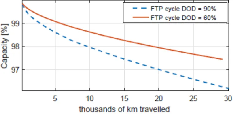
Figure 2Effect of current limitation on cell capacity, DOD fixed to 60% ... 1
Figure 3Effect of DOD on cell capacity without current limitation ... 1
Figure 4Stochastic driving cycle Vs original driving cycle ... 2
Figure 5 Scheme of the fully electric vehicle model ... 3
Figure 6 Li-ion Battery ... 5
Figure 7 Aging Model ... 6
Figure 9Severity factor map ... 8
Figure 10 Chosen parameterization of weight used to penalize low and high SOC ... 9
Figure 11Equivalent circuit ... 10
Figure 12Nissan leaf Vehicle load Curve ... 11
Figure 13 Power Train Model ... 13
Figure 14 Thermal Management ... 14
Figure 15 Comparision of thermal management ... 15
Figure 17Effect of current limitation on speed reference tracking ... 19
Figure 18 TPM Construction ... 24
Figure 19 Sub-matrix graph... 25
Figure 20 TPM Construction ... 26
Figure 21 Cycle generated-A ... 27
Figure 22 Cycle Generated-B ... 28
Figure 23 Pso algorithum ... 34
Figure 24 Flow chart of PSO algorithm ... 35
Figure 25 Time history of the optimal control variable ... 38
Figure 26 graph and table for differnt swarm size and stall iteration-2 ... 41
Figure 27 Graph and table for different swarm size and stall iteration -5 ... 42
8
CHAPTER 1
INTRODUCTION
1.1 INTRODUCTION
The next few years will be a period of further maturation of the electric vehicle industry, nurtured by government support. As a result of tightening vehicle emission regulation and extraordinary government incentives are motivating automakers effort in research and development in the powertrains, with electrified alternatives to ICE and hybrid. The main drawback of the electric vehicle is the limited driving range, relatively slow recharge time and high cost compared to traditional fuel-based vehicles. The high cost is mostly influenced by the battery pack and its replacement during the lifetime of the vehicle: an unresolved challenge is to match the
9
Lifetime of the battery with the life of the vehicle. The current level is generally high. Thus, a controller must manage the electricity requirement for each electric component. To achieve the desired performance and to prevent the possible abnormal operation. One of the main problem electric vehicles are facing is battery related issues, currently available options for batteries in electric vehicles are lead-acid batteries, nickel- metal hydride batteries, sodium-nickel-chloride batteries (also called ZEBRA batteries), and lithium-ion batteries. Lithium-ion batteries are the most common type of batteries for transportation applications, because of its high specific energy, high specific power, good lifespan attributes and low memory effect, they are currently the most commonly used battery technology in modern EVs.
Generally in batteries many different and complex aging mechanisms can be identified during batteries lifetime, but macroscopic effects of battery aging lead to loss of total storage capacity and the increase of the internal resistance, see[1] in general, battery aging can be divided into two main categories: calendar aging and cycle aging. Calendar aging is associated with the energy storage and it occurs even if the vehicle is not utilized. On the other hand, cycle aging is related to battery utilization (battery charge and discharge) and it strongly depends on how the battery is used. Due to the complexities of the electrochemical phenomena involved in the aging process, most of the studies regarding battery cycle aging are empirical studies [2]-[5]. In these works, battery cells are continuously cycled under different conditions and semi-empirical models are derived from the collected data relating battery loss of capacity to various stress factors like temperature, voltage, SOC, and current. It is well established that temperature, Depth of Discharge (DOD), and C-rate are the main stress factors for Lithium-ion batteries. This means that cycling a cell at high C-rate, high temperature and at high DOD makes the cell degrade faster.
1.2 SCOPE AND INNOVATION:
In this thesis, the idea of controlling in closed-loop the capacity loss of FEV battery is explored. Given that a measure of the remaining battery capacity is available, two control actions can be identified in this way: 1) setting the maximum admissible current Imax that can be drawn from the battery in order to dampen the current peaks 2) limit extreme battery DOD, acting on the vehicle charging management. Ideally, one would like to minimize the capacity degradation but this objective is in contrast with some desired performance of the vehicle in terms of acceleration, driving range and
10
charge time. Therefore, the control objective can be defined as controlling the capacity
degradation during the vehicle use and, at the same time, guaranteeing acceptable vehicle performance.
Other contribution of this paper consists in the development of control-oriented FEV model that can be used to understand and quantify the trade-off existing between limiting the battery usage in terms of maximum current Imax and DOD and the vehicle performance. The battery thermal management is also included in the model. Additionally, the thesis also deals with the parameterizing driving cycle, because vehicle driving cycles have a great effect on vehicle performance. If a vehicle manufacturer focuses only on a fixed driving cycle there is a risk that controllers of the vehicles are optimized for a certain driving cycle and hence sub-optimal solutions to real-world driving. To deal with this issue, a new method called Markov process which is based on stochastic process and probability theory is used to generate different driving cycle.
Furthermore, an offline optimization procedure of the control variables is carried out to get some vision of the aforementioned trade-off and to set-up an optimal benchmark for future implementation of online control strategies. Therefore, to realize accurate battery states estimation and improve the performance of EVs, it is necessary to understand the temperature, aging uncertainties to Li-ion battery modeling the techniques of overcoming these uncertainties.
1
1.3 ORGANIZATION OF THE THESIS
This thesis is organized as follows:
In chapter 2, a complete vehicle model able to quantify the effect of different driving situations on battery aging. There are three main sub-models that describe the longitudinal dynamics and the powertrain of the vehicle, the battery cell model that describes the capacity loss of the battery cell depending on the driving conditions and the thermal management module that calculates the power requested to cool down the battery. In addition to this, simulations results which are presented to demonstrate the effect of the control variables (Imax and DOD) on battery capacity loss and vehicle performance.
FIGURE 2EFFECT OF CURRENT LIMITATION ON CELL CAPACITY, DOD FIXED TO 60%
2
Chapter 3 presents a novel methodology to generate stochastic driving
cycles for the design and control optimization of an electric vehicle because using a fixed driving cycle has some sub-optimality where there is a repeatability of same data. To deal with the sub-optimality issue, it is beneficial to have a method for generating more driving cycle that in some sense are equivalent but not identical using an approach based on a multi-dimensional Markov chain.
FIGURE 4 STOCHASTIC DRIVING CYCLE VS ORIGINAL DRIVING CYCLE
Chapter 4, Introduce the Control problem in the optimization framework
using PSO. A Particle Swarm Optimization (PSO) has been used to solve the series of optimization problems using significant tuning parameters like swarm size, stall-iteration. The results of the optimization are carried out in fixing the weight factor and after we find the sensitivity of the weight fact we analysis the control variable with respect to time by changing the control horizon.
3
CHAPTER 2
SYSTEM MODELLING
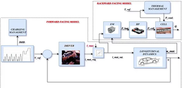
This chapter discusses the modeling approach for the vehicle. The level of acceptable approximation in modeling process defines the efficiency of the model. In order to evaluate the energy economy of the vehicle, it is necessary to understand the energy flow in different powertrain components of the vehicle. The vehicle energy consumption for a prescribed driving cycle can be estimated using backward and forward modeling approach. Where backward-facing modeling takes the assumption that the vehicle meets the target performance, and calculates the component states. Forward facing modeling, on the other hand, simulates the physical behaviors of each component with control instruction, handles state changes, and generates vehicle performance as output. Differently, from this classical approach, the model developed in this work is characterized by a mixed forward-backward facing approach as shown in the figure 5 below:
4
2.1ELECTRIC VEHICLE MODELING
The majority of the works regarding powertrain sizing and energy management utilize a backward-facing approach to model the vehicle. In backward approaches, the desired speed is imposed on the vehicle and the motor speed, torque and power are calculated backward. Differently, from this classical approach, the model developed in this work is characterized by a mixed forward-backward facing approach as highlighted in the figure above. The forward-facing art consists of the modeling of the driver’s response to the desired speed reference and in the modeling of the longitudinal dynamics of the vehicle. The backward-facing part, based on the power requested to run the vehicle, computes in a backward manner the power that is drawn from the battery. Such an approach turned out to be necessary for the framework used in this thesis since the basic assumption that the vehicle is able to meet the speed profile of the driving cycle does not hold. The reader is referred to [11] for more details on forward-facing and backward-facing vehicle simulation. The model of the driver is a simple PI regulator that requests a certain torque to the electric motor based on the speed error e = vref - v. Knowing the motor torque constant kt, The motor current can be directly derived from the torque as ireq = τreq/ kt. The requested motor current is then saturated to a maximum value Imax that, is considered as a control variable to limit the battery current at the cost of limiting also the vehicle acceleration. The motor current is then used to calculate vehicle speed according to the longitudinal vehicle dynamic equation:
𝑚𝑑𝑣 𝑑𝑡 = 𝑖𝑚𝑜𝑡𝑠𝑎𝑡 𝑘𝑡𝑘𝑔 𝑅𝑤 − 1 2𝜌𝑣 2𝐶 𝐷𝐴 − 𝐹𝑟𝑜𝑙𝑙
where Kg is the gear ratio, Rw is the wheel radius, Froll is the rolling resistance, CD and A are the drag force coefficient and the cross-sectional area respectively.
5
2.2BATTERY CELL:
LITHIUM-ION BATTERIES:
Lithium-ion batteries are the most common type of batteries for transportation applications due to high specific energy, high specific power, good lifespan attributes and low memory effect, they are currently the most commonly used battery technology in modern EVs.
LITHIUM-ION BATTERIES FUNCTION :
A lithium-ion battery is a rechargeable battery in which lithium ions move between the anode and cathode, creating electricity flow useful for electronic applications. In the discharge cycle, lithium in the anode (carbon material) is ionized and emitted to the electrolyte. Lithium ions move through a porous plastic separator and insert into atomic-sized holes in the cathode (lithium metal oxide). At the same time, electrons are released from the anode. This becomes electric current traveling to an outside electric circuit
FIGURE 6 LI-ION BATTERY
When charging, lithium ions go from the cathode to the anode through the separator. Since this is a reversible chemical reaction, the battery can be recharged. A lithium-ion battery cell contains four main components: cathode, anode, electrolyte, and separator. Table 1 shows the main components’ functions and material compositions.
6
Table 1 COMPONENTS OF LI-ION BATTERY
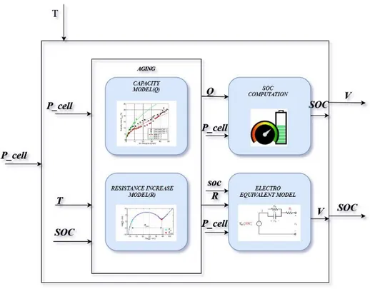
2.3 BATTERY CELL MODELLING:
FIGURE 7 AGING MODEL
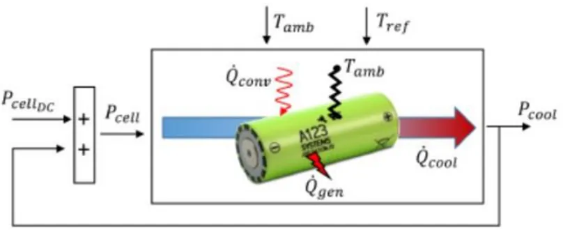
The batteries electric and thermal behavior should be considered in the cell model. The inputs to the cell model are the requested power to the cell
7
blocks they are an electrical equivalent circuit, aging model, and SOC computation as shown in figure 7
2.4 AGING MODEL:
The aging model is inspired by the experimental identified in [2”G.suri and S.onori “A control-oriented cycle-life model for hybrid electric vehicle Li-ion batteries]. It is formulated here as a non-linear differential equatLi-ion describing the rate of capacity loss with respect to the Ah processed.
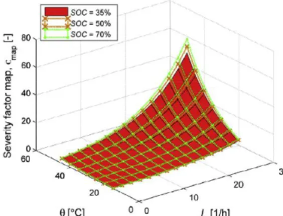
According to the above equation, three stress factors influence the battery degradation: cell temperature T, C-rate Ic defined as the operating current normalized by the nominal cell capacity Qnom and SOC. Regarding the effect of current rate on battery, aging is considered as more than the effect of temperature and SOC. Ref[2]where it shows a graph fig where the curvature of severity factor (σmap) increases significantly with Ic. This implies that the aging of the battery is accelerated under high Ic values. A high-stress zone and low-stress zone are defined on the map in order to differentiate between different severity conditions with respect to different degrees of aging.
8
FIGURE 8 SEVERITY FACTOR MAP
Temperature has two different effects on the battery's performance. As temperature increases the efficiency of the battery increases due to the decrease in battery equivalent internal resistance. Simultaneously, it also aggravates battery aging by accelerating the rate of unwanted side reactions, leading to the growth of SEI layer on the electrodes. As shown, the severity factor map rises with temperature. As shown in fig 8 are the severity factor maps for three different values of SOC that almost overlap with each other over the domain of chosen values for Ic and ϴ. But the SOC has a very little effect on battery degradation. This result can be explained by the fact that the considered range of SOC was limited to 30-75% that is the reasonable operating range for a hybrid electric vehicle where the supervisory control runs the internal combustion engine at very low and very high SOC.
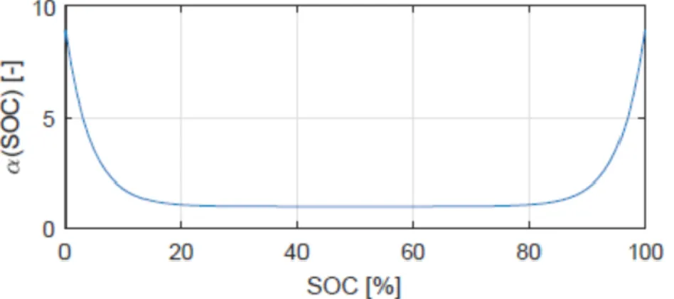
In the case of FEVs, it is important to account for the effect of high and low SOC on battery aging in case the driver wants to exploit the full capacity of the battery to extend the range of the vehicle. Previous works such as [5] and [13]showed that significant depths of discharge that leads the battery to operate below 20% and above 80% of SOC affect the battery aging for this reason the aging model includes the penalizing factor α_soc in order to provide a faster aging rate at high and low soc.
9
Where c,b,soc_min and soc_max are tuning parameters that can be used to shape the penalization function and that is practice, should be identified through ad-hoc aging experiment parametrization of α_soc chosen in this work. Besides the loss of capacity, battery aging results in an increase of the internal resistance R, Inspired by the experimental results published in[14] a linear relationship between resistance increment delta R and capacity decrement deltaQ
FIGURE 9 CHOSEN PARAMETERIZATION OF WEIGHT USED TO PENALIZE LOW AND HIGH SOC
2.5 ELECTRO EQUIVALENT CIRCUIT MODEL:
There have been many attempts to develop battery models. The most common models are the electrochemistry model and the electric circuit model. While detailed chemistry-based models have been built to investigate the internal dynamics of batteries, these models are generally not suitable for the design of electrical systems. On the other hand, circuit-based models have been built in terms of electric-circuit parameters, such as capacitances, resistances, voltage sources, etc.
10
FIGURE 10 EQUIVALENT CIRCUIT
Here equivalent circuit model has the advantage of a simple structure and a clear physical concept.OCV can accurately reflect SOC. If OCV could be observed accurately it should be possible to very accurately estimate SOC. The circuit contains an ideal power source, an internal resistance, and an equivalent RC network .The open circuit voltage V, and the estimation of the state-of-charge (SOC) are the outputs of the electrical model
Open Circuit Voltage The open circuit voltage (OCV) of the battery is the stable voltage value of the battery when the battery is left in the open circuit condition [11]. Regarding the battery after being charged, the battery terminal voltage will gradually decline to a stable value when it is left in the open circuit condition; regarding the battery after discharge, the battery terminal voltage will gradually rise to a stable value after the load is removed. The electromotive force of the battery is basically equal to the open circuit voltage of the battery, while the battery electromotive force is one of the metrics used to measure the amount of energy stored in the battery. Thus, there is a certain relationship between the battery OCV and the battery SOC [22]. There are a few ways to obtain OCV, in which the stationary method is a direct method and is relatively more accurate
11
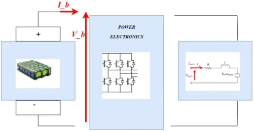
The battery is modeled by an equivalent circuit comprising a voltage source Vcc and its internal resistance R0 in series, and both variables are functions of the SOC. Thus, the battery current is given by
𝑃𝑏𝑎𝑡𝑡is the power in and out of the battery. SOC is computed from the battery current as
𝑄
𝑏𝑎𝑡𝑡is the battery capacity. In addition to SOC, battery
temperature is also a state of the battery system model. However,
in the optimal control system, temperature is not considered as a
state assuming that an independent battery thermal management
system will keep the battery temperature at a known desired value.
2.7 VEHICLE CHARACTERISTICS:
12
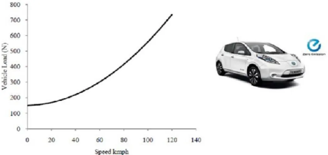
For the study, Nissan leaf vehicle parameter powertrain model assumption is made on the various components. The vehicle load force, F, as determined can be estimated on the coefficients A, B, and C published by the EPA and provided in[2] for many vehicles including several EVS and is as follows:
Where u is the vehicle speed.
The plot of vehicle load force VS speed is shown. Such a curve can also be easily generated using data for the vehicle drag coefficient and rolling resistance, as done in [4]. However, the coast-down data curve is really useful as it contains additional speed-related losses within the vehicle drivetrain in addition to all the external load forces such as drag and rolling resistance.
2.8.POWER TRAIN :
The power that the electric motor has to provide can be calculated from torque and speed:
𝑃𝑚𝑜𝑡 = 𝐾𝑡𝑖𝑚𝑜𝑡𝑠𝑎𝑡𝑣
13
FIGURE 12 POWER TRAIN MODEL
In a backward facing approach, the motor is modelled as a simple efficiency map depending on torque and speed, therefore the power requested to the battery to perform the driving cycle can be calculated dividing the motor power by the motor efficiency:
𝑃𝑏𝑎𝑡𝑡𝐷𝐶 = 𝑃𝑚𝑜𝑡
𝜂𝑚𝑜𝑡(𝑘𝑡 𝑖𝑚𝑜𝑡𝑠𝑎𝑡, 𝜔𝑚𝑜𝑡)
The power requested to the battery needs to be scaled down to the single cell based on the number of cells present in the battery pack. The battery cell considered in this work is a commercial A123 cylindrical LiFePO4 cell characterized by a nominal voltage of 3.3 V and a nominal capacity of 2.5 Ah. This particular cell has been chosen as a reference because it is very well studied in the literature, nevertheless, the modeling approach used here is general and, if accordingly parametrized, can be applied to any other Li-ion cell. In order to match the voltage and total energy of the Nissan Leaf battery pack, 2910 A123 cylindrical cells need to be used. The DOD of the battery is controlled through the charging management module: when the control schedule a charging event, the charging management block modifies the driving cycle in order to stop the vehicle and perform the charging of the battery.
14
2.9 THERMAL MANAGEMENT
Li-ion battery is very vulnerable in overheated environments during high C rate HEV operations. If the heat is accumulated in the battery package, the temperature exceeds certain limitations, which might lead to serious battery failure. Especially considering that high temperature will reduce the electric
resistance at the battery electrode end, an even larger current might be
resulted and leads to a higher heat generating rate. Therefore, the battery temperature should be strictly controlled within a narrow margin and avoid this kind of thermal runaway. Forced air or liquid cooling is required 48 in EV/HEV’s battery modules to effectively remove the heat.
The Li-ion battery cells are sensitive to temperature changes. Consequently, their performance will be significantly reduced if the internal chemical reaction cannot proceed in a proper temperature range. Long time operation under overheated conditions will also decrease the battery cycle life. Here we have a control scheme of the thermal management to keep the temperature of the cell at a certain reference temperature and two types of heat are considered one generated by the cell and other from the atmosphere
15
Electric power is equal to total amount of heat to be dissipated over coefficient of the performance of the heater or cooling system. This control theory is introduced to track the reference temperature by minimizing the temperature fluctuations. We are using a thermal management that consumes some current to keep the temperature and this current is requested from the driving cycle and some current from the thermal management.
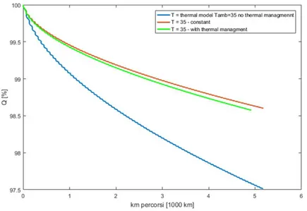
FIGURE 14 COMPARISION OF THERMAL MANAGEMENT
There are 3 cases in the graph
Case 1: Without a thermal management system (blue) – a variation of temperature is high. For an instant, if we some certain temperature in the ambient, the temperature starts increasing drastically
Case 2: With thermal management system (green)-the temperature is kept constant by the thermal management system. This thermal management system draws additional current. In order to keep the battery cool we have to pay for extra energy .so the thermal management system will draw additional current.
16
Case 3: We assume to have the ideal thermal management (red) Ideal thermal management is you don’t pay the extra cost in terms of current. The battery temperature is kept at 35 degrees. This allows quantifying additional current we have to draw to keep the battery at 35 degrees constant
2.10 IMPORTANT TERMS:
Various terms have been defined for batteries to characterize their performance. Commonly used terms are summarized in the following as a quick reference.
State of Charge (SOC) It is a percentage of instantaneous battery capacity left out of total battery capacity. SOC can be calculated by integrating battery current over a period of time.
Depth of Discharge (DOD) the percentage of battery capacity discharged in the terms of total capacity is known as depth of discharge. Generally, DOD can be related to SOC as follows;
DOD = 1−SOC
Cell, Module, and Pack A single cell is a complete battery with two current leads and separate compartment holding electrodes, separator, and electrolyte. A module is composed of a few cells either by physical attachment or by welding in between cells. A pack of batteries is composed of modules and placed in a single containing for thermal management. An EV may have more than one pack of battery situated in a different location in the car.
C-rate C (nominal C-rate) is used to represent a charge or discharge rate equal to the capacity of a battery in one hour. For a 1.6 Ah battery, C is equal to charge or discharge the battery at 1.6 A. Correspondingly, 0.1C is equivalent to 0.16 A, and 2C for charging or discharging the battery at 3.2A.
17
Specific Energy Specific energy, also called gravimetric energy density, is used to define how much energy a battery can store per unit mass. It is expressed in Watthours per kilogram (Wh/kg) as
Specific Energy = Rated Wh Capacity/Battery Mass in kg
The specific energy of a battery is the key parameter for determining the total battery weight for a given mile range of EV.
Specific Power Specific power, also called gravimetric power density of a battery, is the peak power per unit mass. It is expressed in W/kg as
Specific Power = Rated Peak Power/Battery Mass in kg
Energy Density Energy density also referred to as the volumetric energy density, is the nominal battery energy per unit volume (Wh/l).
Power DensityPower density is the peak power per unit volume of a battery (W/l).
Internal Resistance Internal resistance is the overall equivalent resistance within the battery. It is different for charging and discharging and may vary as the operating condition changes.
SOC is a critical condition parameter for battery management. Accurate gauging of SOC is very challenging, but the key to the healthy and safe operation of batteries.
State of Health (SOH) SOH can be defined as the ratio of the maximum charge capacity of an aged battery to the maximum charge capacity when the battery was new [7]. SOH is an important parameter for indicating the degree of performance degradation of a battery and for estimating the battery remaining lifetime.
18
2.11 SIMULATION RESULTS:
It is difficult to validate a battery aging model on real vehicle data because an ad hoc experimental campaign is very costly and time-consuming. In order to give a rough idea of the model validity, the capacity degradation calculated by the proposed model is compared with some experimental data published online. Despite the great number of vehicle parameters published online for the Nissan Leaf, no clear experimental analysis has been found regarding its battery aging. Therefore the capacity loss predicted by the proposed model has been compared with experimental data published in for the Tesla Model S.
The model is run over a mixed urban-highway Artemis cycle at a constant temperature of 30 degrees Celsius.figure15 shows how the capacity calculated by the model reproduce reasonably well the capacity loss of the Tesla battery. This comparison should be intended as a reasonableness check other than a rigorous model validation.
15FIG-MODEL CAPACITY DEGRADATION SIMULATED OVER A MIXED URBAN HIGHWAY ARTEMIS CYCLE COMPARED TO TESLA MODEL S EXPERIMENTAL DATA
In the following, some simulations results are presented to demonstrate the effect of the control variables Imax and DOD on battery capacity loss and vehicle performance. In a first approximation, it is possible to relate the maximum motor current to the maximum allowable cell current through the following power balance:
19
𝐼𝑚𝑎𝑥 =𝐼𝑚𝑎𝑥𝑐𝑒𝑙𝑙𝑉𝑐𝑒𝑙𝑙𝑛𝑜𝑚𝑛𝑐𝑒𝑙𝑙
𝜔𝑚𝑜𝑡𝐾𝑡𝜂
where η is an average electric motor efficiency. Therefore, in the following, the maximum allowable cell current 𝐼𝑚𝑎𝑥𝑐𝑒𝑙𝑙 is considered as a control variable that can be translated in a maximum motor current through the approximated relation described by Figure 2 shows the effect of limiting the maximum current drained from the battery during a simulation where the electric vehicle performed the US Federal Test Procedure (FTP cycle) for a total distance of 30000 km. The result is that, for the same travelled distance, limiting the maximum current at 0.75 C helps in limiting the loss of battery capacity: at 30000 km there is a 0.25% of capacity saved that corresponds to an improvement of 10% with respect to the nominal case without current limitation. There is a price to pay in controlling the maximum current: limiting the maximum current means limiting the maximum acceleration during driving and slows down the charging process.
FIGURE 16EFFECT OF CURRENT LIMITATION ON SPEED REFERENCE TRACKING
The figure16 shows the actual speed profile of the vehicle compared with the FTP reference speed: It is clear how, limiting the current, the vehicle is not able to follow the reference during demanding accelerations especially at high speeds. It is important to remark that the effect of limiting the maximum current on cell capacity is strictly dependent on the driving cycle: for the same maximum limit Imaxcell, if the speed profile is very demanding
20
in terms of accelerations, the benefit on the capacity will be relevant. In case the speed profile is so smooth that the current request rarely exceeds the limit, the effect will be almost negligible. Figure 3 shows the effect of DOD on cell capacity. It can be seen that reducing the DOD down to 60% can save 1% of battery capacity in the first 30000 km. The price to pay in this case is that the range is substantially reduced because 40% of the capacity of the battery is not exploited at all. As a side effect, the charging time is reduced. In the considered situation, it can be noted that limiting the DOD has a more evident effect on battery aging compared to setting a limit on the maximum current: this fact is a peculiarity of FEV compared to hybrid vehicles. In hybrid powertrains, the battery size is much smaller since it does not have to guarantee a long driving range but the battery is subject to higher currents in order to power the entire vehicle in EV mode. Furthermore DOD usually has a small influence in hybrid vehicles because the supervisory controller never runs the battery at extreme SOC values. On the other hand FEV are designed with large battery packs resulting in smaller cell currents and therefore a smaller current sensitivity on battery degradation.
21
CHAPTER 3
DRIVING CYCLE GENERATOR
This chapter analyzes electric vehicle behavior, its impact based on using a standard driving cycle. A driving cycle also called driving schedule or speed profile is a representation of vehicle speed versus time. Vehicle driving cycles have a great effect on the vehicle performance. In the above chapters, we use a single certification cycle, which is repeated many time to assess the performance over specific kilometers, as a drawback, applying single driving cycle create sub-optimality, this way we drop some performance in the real world. In order to fix this problem, Markov based approach which is based on stochastic process and probability theory is used. This chapter contains the generation of driving cycle including the process of construction of transition probability matrices (TPM) and uses the TMP matrix to generate the driving cycle.
DRIVING CYCLE GENERATION PROCEDURE
3.1 Markov process
Markov Process Markov process theory defines a particular type of stochastic process. The generation procedure uses Markov chain due to its simplicity in representing an unknown system. Having the Markov property means that future states depend only on the present state and are independent of the past states. A Markov chain is a sequence of random variables X1, X2, X3,...with the Markov property as expressed as
22
The set of possible values that the random variables Xn can take is called the state space of the chain. The conditional probabilities pij :=P(Xn+1 = j|Xn = i)are called transition probabilities. The probability used in the synthesis procedure is time independent. The sum of all probabilities leaving a state must satisfy
The states required to satisfy the Markov property are determined based on the assumption that the vehicle dynamics can be simplified using the following dynamic equation:
Fnet=Fprop−FRR−FWR−FGR
where Fnet is the net force applied to the vehicle, Fprop is the propulsion force from the powertrain, FRR is the rolling resistance force, FWR is the wind resistance force, FGR is the grade resistance force and all other external forces applied to the vehicle. Vehicle dynamics can be represented using two states, namely: 1) vehicle velocity and 2) acceleration. Thus, we select them as the states for the Markov chain.
The methodology based on the Markov process theory mainly consists of three steps to generate the driving cycle. Here we use UDDS (city) and HWFET (highway)
1. Discretization of velocity and acceleration profile 2. Construction of transition probability matrix(TPM)
3. Generating the driving cycle
3.2 DISCRETIZATION OF VELOCITY AND ACCELERATION:
In order to generate a TPM matrix, there is a need to discretizing velocity and acceleration into a number of time steps. Here we use UDDS(city) and HWFET(highway) driving cycle to see the performance difference. Below table shows the driving profile discretization in steps of:
23
TYPE STEPSIZE
velocity 1.0km/h
acceleration 0.2m/s^2
Characteristics of driving cycle :
3.3 TPM construction:
The TPM matrix contains probabilities to transition from one state to another state. Each state is defined by the state variables, velocity, and acceleration. To increase the readability, the TPM is constructed as a large matrix containing smaller sub-matrices, as seen in Figure17:
HWFET Duration: 765 seconds Total distance:16.45Km Average speed:77.7km/h UDDS Duration:1372 Total distance:12.07Km Average speed:31.5Km/h
24
FIGURE 17 TPM CONSTRUCTION
Each state corresponds to a specific element in the TPM, that contains a smaller matrix with the transition probabilities. The size of the large matrix is determined by the maximum velocity and the absolute maximum acceleration combined with the resolutions for velocity and acceleration. The number of rows, nr, and columns, nc, are calculated using:
For example, if the maximum velocity is 180 km/h, and the resolution is 1 km/h, there will be 181 columns. If the absolute maximum acceleration is 8.2 m/s^2, and the resolution is 0.2 m/s^2, there will be 83 rows in the TPM. The first column in the matrix corresponds to zero velocity and the middle row to zero acceleration. This way first we build the empty large matrix.
25
3.4 PROCEDURE TO PACK EACH SUBMATRIX:
First, the velocity and acceleration data of the selected driving cycles are gathered. Then, the TPM is generated in the form of a 2-D matrix. Once we discretize both velocity and acceleration profile, there will be a specific time point where both velocity and acceleration points fall within a specific time limit you are considering as shown in the figure. (blue-time when velocity inside the bin,green-time when acceleration inside the bin,red-times when both inside the respective bin).After selecting time tk we have to select time tk+1 which is the time next to the point. This way it steps through each input driving cycle and saves state transition in the correct sub-matrix. A new row is added to the sub-matrix for each time a state is visited, changing the size of the submatrix.
When all driving cycles have been sorted into the TPM, there is a need to sort and summarize the sub-matrices. A value of how many times a unique
26
transition has occurred is calculated and the transition probabilities are derived.
Probability = count of each unique pair/number of time points in total
The TPM is constructed as a Matlab structure using Matlab code since there is a need to store different kinds of data within it.
FIGURE 19 TPM CONSTRUCTION
In each cell of the TPM, the probability matrix of the velocity and the acceleration at the next time tk+1 are included. Each cell represents the conditional probability
P(vk+1 = v2,ak+1 = a2|vk = v1,ak = a1) at a given cycle velocity and acceleration. As an example, starting at a state characterized by 41 mi/h and 0.2 m/s2, the probability of acceleration increasing in the next step to 0.4 and velocity to 42 mi/h is 0.343, while the probability of cruising at exactly the same speed with zero acceleration is only 0.0132.
27
3.5DRIVING CYCLE CONSTRUCTION
When a TPM has been created, it is possible to start generating driving cycles. The process starts by calculating the desired driving cycle duration. The process starts in the idle state (zero velocity and acceleration). The first transition is leaving the idle state and the driving cycle is then built up through generating a random number. whenever the random number is less than the cumulative probability of individual bin choice them we jump to that bin and record it at the next time step. The iterative process continues until the desired duration is exceeded at the same time as the end state has a velocity equal to zero.
3.6 RESULTS OF DRIVING CYCLE GENERATOR:
The driving cycle is generated for two scenarios:
One for the city (UDDS) and other for HWFET(highway).The original driving cycle is in blue line and the stochastic driving cycle is in red line.you can see the graph generated looks
28
This way for each simulation we get different driving cycle by changing the TPM value each time. Here we are presented for two different driving style.
29
CHAPTER 4
OPTIMIZATION FRAMEWORK AND PSO
Optimization is an important activity in many fields of science and engineering. A lot of modeling, design, control and decision making problems can be formulated in terms of mathematical optimization. The classical framework for the optimization is the minimization (or maximization)of the objectives, given the constraints for the problem to be solved. Many design problems, however, are characterized by multiple objectives, where a trade-off amongst various objectives must be made, leading to under or over-achievement of different objectives. Our broader idea is to create a closed loop optimization controller, by setting the reference for the future driving cycle using Markov based process. In this chapter, to manage the battery degradation in EV we have to consider several trade-offs. It is interesting to further analyze the trade-off in an offline optimization framework, which helps in real-time. In order to create an optimal benchmark for online control strategies.
4.1 PERFORMANCE INDEX AND OPTIMIZATION HORIZON:
Define four indexes of performance: Jlife, Jspeed, Jcharge, Jrange. Consider an optimization horizon during horizon only the first element of the optimal control sequence is applied. In the vehicle, the SOC varies as we use the energy, here you let the driver accelerate and at each control horizon the algorithm will decide what is the maximum current allowed and how much the driver is allowed to cycle. At the next time steps, the prediction horizon
30
moves forward and the process is repeated. In each control horizon, Imax and DOD are optimized to minimize the cost function of the equation.
Considering an optimization horizon [0; tend], we can define Jlife as the capacity degradation over the considered time horizon normalized by the traveled kilometers:
𝐽𝑙𝑖𝑓𝑒 =Q(0) − Q(tend) ∆km
Jspeed is defined as the root mean square value of the speed difference between the cycle reference and the actual speed of the vehicle:
Jspeed= √𝑡1
𝑒𝑛𝑑∫ (𝑣𝑟𝑒𝑓 (𝜏) − 𝑣(𝜏)
𝑡𝑒𝑛𝑑
0 )
2𝑑𝜏
This index represents the driveability of the vehicle. Jcharge and Jrange are the root mean square values of the charge time and driving range calculated over the charging events in the considered time horizon:
Jcharge=√1
𝑁∑ 𝑡𝑐ℎ𝑎𝑟𝑔𝑒(𝑖) 2
𝑁 𝑖=1
31 Jrange=√1 𝑁∑ 𝑟𝑎𝑛𝑔𝑒 2 𝑁 𝑖=1 (𝑖)
where N is the total number of charging events performed on the horizon. During the vehicle life, ideally one would like to minimize the battery aging Jlife and the charge time Jcharge, maximize the driving range Jrange and to perfectly follow the speed reference i.e. minimizing Jspeed .
Of course, this objective functions are in contrast with each other and more specifically, the minimization of Jlife is in contrast with the other terms. The multi-objective optimization problem can be reduced to a single-objective optimization problem that consists in finding the optimal control variables DOD, Imax_cell to minimize a weighted summation of the various terms:
Jtot=αchargeJcharge + αspeedJspeed – αrangeJrange + αlifeJlife
Depending on the weight αlife, αcharge, αrang, αspeed one can give more importance to one or more aspects of the problem over the other.
4.2 WITHOUT APPLYING OPTIMIZATION ALGORITHM:
Below you can see the aging of the battery without applying the optimization algorithm.
32
FIGURE 22 WITHOUT CONTROL STIMULATION
This is the result of the stimulation which represents the cost function given above, here we consider 30-hour experiment.
J
charge-Each point in the graph represents a single charge. Every 3 hour wehave to recharge that recharging time takes 45 min which depends on SOC.
J
range-Each point represents the range we are able to cover in every single charge.J
life–In 30 hours we lose 0.01 Ah. This is the one we use in the cost functionJ
speed-This is the difference between drivers request and real speed of the vehicle.This graph is not an optimization model, here it just shows the aging of the battery using an experiment
4.3 OPTIMIZATION METHOD
The objective of this study is to quantify the trade-off between battery aging and performance of the vehicle. Weight factor αlife, αrange, αspeed, αcharge are
33
chosen to make Jlife , Jspeed, Jcharge, Jrange have the same weight in the cost function. While the optimization has been performed several times with different values of αl, followingly check the optimization performance of the control variable over time.
In the first method different value of αlife, a total horizon of 30,000 km of the FTP cycle and a control horizon of 3000 Km have been chosen for the optimization. On the other hand, the specific position of αlife is secured for a control horizon of 1000 Km of the ‘ArtRoad’ cycle is considered. In practice, in each control horizon, Imax and DOD are found to minimize the overall cost function given below:
4.4 OPTIMIZATION SOLUTION IS SOLVED USING PSO
Particle swarm optimization (PSO) algorithms are nature-inspired population-based metaheuristic algorithms originally accredited to Eberhart, Kennedy, and Shi. These algorithms mimic the social behavior of birds flocking and fishes schooling. Starting to form a randomly distributed set of particles (potential solutions), the algorithms try to improve the solutions according to a quality measure (fitness function). The improvisation is performed by moving the particles around the search space by means of a set of simple mathematical expressions which model some interparticle communications. These mathematical expressions, in their simplest and most basic form, suggest the movement of each particle toward its own best-experienced position and the swarm’s best position so far, along with some random perturbations.
34
PSO Algorithm works :
The PSO algorithm works by simultaneously maintaining several candidate solutions in the search space. During each iteration of the algorithm, each candidate solution is evaluated by the objective function being optimized, determining the fitness of that solution. Each candidate solution can be thought of as a particle “flying” through the fitness landscape finding the maximum or minimum of the objective function. Initially, the PSO algorithm chooses candidate solutions randomly within the search space. The figure shows the initial state of a four-particle PSO algorithm seeking the global maximum in a one-dimensional search space. The search space is composed of all the possible solutions along the x-axis; the curve denotes the objective function. It should be noted that the PSO algorithm has no knowledge of the underlying objective function, and thus has no way of knowing if any of the candidate solutions are near to or far away from a local or global maximum. The PSO algorithm simply uses the objective function to evaluate its candidate solutions and operates upon the resultant fitness values.
35
Each particle maintains its position, composed of the candidate solution and its evaluated fitness, and its velocity. Additionally, it remembers the best fitness value it has achieved thus far during the operation of the algorithm, referred to as the individual best fitness, and the candidate solution that achieved this fitness referred to as the individual best position or individual best candidate solution. Finally, the PSO algorithm maintains the best fitness value achieved among all particles in the swarm, called the global best fitness, and the candidate solution that achieved this fitness called the global best position or global best candidate solution.
Figure 24 Flow chart of PSO algorithm
The PSO algorithm consists of following steps, which are repeated until some stopping condition is met.
1. Evaluate the fitness of each particle
36
3. Update velocity and position of each particle. The first two steps are fairly trivial. The fitness evaluation is conducted by supplying the candidate solution to the objective function. Individual and global best fitnesses and positions are updated by comparing the newly evaluated fitnesses against the previous individual and global best fitnesses and replacing the best fitnesses and positions as necessary. The velocity and position update step is responsible for the optimization ability of the PSO algorithm. The velocity of each particle in the swarm is updated using the following equation:
4.5 BASIC TUNING PARAMETER OF PSO ALGORITHM :
Fundamentals of the PSO technique are stated and defined as follows:
SwarmSize: Number of particles in the swarm, an integer greater than 1.
SelfAdjustmentWeight(c1): Weighting of each particle’s best position when adjusting velocity. A finite scalar with default 1.49
SocialAdjustmentWeight(c2): Weighting of the neighborhood’s best position when adjusting velocity. A finite scalar with default 1.49
MaxIterations: Maximum number of iterations particle swarm takes.
Stall iterations.(eg-for sall iteration 5) Bestfval- Best (lowest) objective function value found.
37
Table 2 STALL ITERATION EXAMPLE
4.6 IMPACT OF WEIGHT FACTORS IN THE COST FUNCTION:
VARYING DIFFERENT αlife:
A Particle Swarm Optimization (PSO) has been used to solve the series of optimization problems using a swarm size of 200 particles. The results of the optimization for different values of αl are summarized in Figure 25
Figure 25 Pareto-front like representation of the battery Vs vechicle performance
38
The first three plots represent the trade-off between Jlife and the other performance indexes, the fourth plot represents the mean values of the optimal control variables over the entire horizon. For low-medium values of αl (green and yellow dots), the optimal control action mainly results in reducing the DOD with a consequent reduction of the driving range. For this range of αl, Imax_cell is also reduced from 3C to 2C causing a slow down of the average charge time. Driveability is not affected in this range since Jlife is reduced without affecting Jspeed: this is due to the fact that the FTP cycle never demands for long periods of time battery currents over 2C, therefore the accelerations performance of the vehicle are not modified. As we increase the weight of battery aging (red dots), the control action results in reducing the maximum current below 1C and in a consequent deterioration of the acceleration performance (Jspeed ). Furthermore, the optimal control variables for a value of αl located at the ’elbow’ of the Pareto curve (yellow-orange dots) are computed over a horizon of 200000 km, a value that usually approaches the vehicle useful life. The control variables along with the capacity loss are plotted in the time domain in Figure26
39
As it can be seen, larger control efforts are used in the first 50 thousand kilometers: DOD is limited below 50 % and the cell current is limited below 2C. After the first 50 thousand kilometers, the optimal DOD and Imaxcell settle around a constant value of 50% and 2.5 C respectively. This behavior is due to the fact that the aging degradation rate is higher for the first thousands Ah processed by the battery, motivating a greater control effort in the first thousands of kilometers compared to the rest of the vehicle life. The capacity plot in Figure shows how the optimal control sequence performs compared to using constant DOD and Imax over the entire vehicle life. A very limited DOD and Imax (es: 40% and 1.5 C respectively) produces the highest remaining capacity but strongly limit the range and the other vehicle performance for the whole vehicle lifespan. More relaxed constraints on DOD and Imax (es: 50% and 2.5 C respectively) allows better performance but results in a higher capacity degradation. The optimal control sequence stands in the middle: it limits the battery stress in the first part of the vehicle life and then reduces the control effort after 50000 kilometers.
4.7 OPTIMIZATION PERFORMANCE ANALYSIS WITH RESPECT TO TIME:
It is important to study how the optimization performance of the two control variable DOD, Imax change over time. The above-discussed results for the simulation for 30,000 km with a control horizon of 3000 km is chosen and found the sensitivity of αl. Here to analyze control variable with respect to time we are fixing the αl and see how the actual value of the cost function changes by varying the control horizon. So, here we consider 1000km as our control horizon(i.e optimal variable changes from 2,4,8). Considering ARTroad driving cycle. There are some parameters set for the optimization framework is given below :
40
Table 3 PARAMETERS FOR OPTIMIZATION
Effect of swarms:
There are different tunning parameter in PSO. In that swarm, size is considered as an important parameter. To study how population size affects both accuracy and optimization time. A small population size provides a small mapping of the search space, possibly resulting in a premature convergence. On the other hand, a large population size will considerably increase the computation effort. So that what study of population size is considered to be an important parameter. Here we have solved the optimization problem by varying the swarm size between 10 to 400 for three different values of stall iteration (i.e 2,5,10). From the table, we can see swarm size between 200 and 250 being an optimal value after that After that the optimal value keep on increasing by increasing the simulation time.
Parameter Settings Swarm size 10,100,150,200,250 Stall iteration 2,5,10 Inertial weight [0.1 , 1.1 ] Self-adjustment weight 1.49 Socialadjustment weight 1.49
41
FIGURE 27 GRAPH AND TABLE FOR DIFFERENT SWARM SIZE AND STALL ITERATION-2
We are repeating the same for stall iteration 5 and 10 by varying the swarm size between 10 to 400. From the results, we could conclude saying that if we keep on increasing the swarm size we don’t get a better accuracy and also we lose simulation time. From the results, we could see 200 seems to be the best optimal population number, swarm size 200 gives a better accuracy and satisfactory simulation time. Also we found from the result that even if we increase the swarm size with less stall iteration number we don’t find an optimal results ,this way we found that Jopt is increasing instead of decreasing, after a while we just keep on increasing the time but we do not get an optimal value(accuracy)but when we try to increase the stall iteration limit we have some satisfactory results . This shows that stall iteration places an important role in finding the optimal population number. To find the global minima of 200 particles is enough. And the optimal value of the cost function is 1239.
42
FIGURE 28 GRAPH AND TABLE FOR DIFFERENT SWARM SIZE AND STALL ITERATION -5
43 4.8 DIVIDE THE CONTROL HORIZON:
After finding the optimal swarm size, which guide to solve the optimization problem by changing the control horizon which by increasing the optimal variable by dividing the control horizon.The optimal variable(i.e 2,4,8) by setting km_end as 1000 km.
Table 4 CONTROL HORIZON STALL ITERATION 5
From the table, we can see that DOD is limited between 33 to 37 % and cell current is limited in a specific bound. for the swarm size 200 and stall iteration 5. As we keep on increasing the optimal variable the, optimal best value also increase this shows that we did not give the particle enough time to reach the optimal position in the search space. So next we tuned the parameter of the stall iteration. In the next simulation, we try to increase the stall iteration to 10.Hence, we give an algorithm much more time to find the best value.
44 USING STALLITERATION 10:
Table 5 CONTROL HORIZON STALL ITERATION 10
From the above table using stalliteration value as 10, the DOD is limited below 40% and the current Imax is limited below a specific bound respectively for the optimized population size 200 and the optimal best value is noted as 1018. This shows that stall iteration plays an important role to find the optimal results. Also when we keep on increasing the predictive horizon we are attaining the global best value.On the other hand, we also lose simulation time.
4.9 VALIDATE THE ABOVE BEST FIT :
In the above discussions we found several optimal values for a different case, but how do we check the how good are our optimal value?
We have control over the optimization parameter. In order to verify our results we have to take a random control variable without using the controller i.e we do not limit the current and on the contrast, we will take a value by using the controller i.e where the current is limited. In order to justify the results, we consider the best value 1239 which is drawn from the figure 25. And found the gain points between without control and with control are fair values.
45
Table 6 GAIN POINTS B/W WITH CONTROL AND WITHOUT CONTROL
DOD for without control without control values Best f(x) value obtained with control(30%dod for the correspondent value) Gain of points between without control and with control Percentage of the gain of points b/w without control to with control 90% 56820 1239 55581 98% 80% 13067 1239 11828 91% 70% 2849 1239 1610 56% 60% 1612 1239 373 23% 50% 1419 1239 180 13% 40% 1320 1239 81 6.1% 30% 1370 1239 131 9.5% 20% 1365 1239 126 9.2% 10% 1325 1239 86 6.4%
46
CHAPTER 5
CONCLUSION AND FUTURE WORK
In this thesis, the problem of controlling in closed-loop, the battery aging of an FEV has been defined. An ad-hoc electric vehicle model has been developed for this specific purpose. Furthermore, the existing trade-off between limiting battery usage in order to mitigate its degradation and vehicle performances has been explored in an optimization framework. The algorithm used to optimize the control variable is using particle swarm optimization(PSO) technic. This offline optimization framework gives us a benchmark that poses the basis for future implementations of online aging management strategies. The result presented for optimization framework was using the driving cycle(FTP). Here we also study about driving cycle, because the driving cycle have a great impact on vehicles performance. This work also, introduces to a novel method to parametrize a driving cycle, required as input in powertrain design studies. The attributes considered is velocity and acceleration using Markov chain theory. Where different driving cycle is generated using TPM matrix. The generated cycle is equivalent to the standard certified driving cycle. This way we can avoid the risk of using the fixed driving cycle and improve the performance of the vehicle by not repeating the same data (i.e) to avoid repeatability in the driving cycle. The result presented here of One for the city (UDDS) and other for HWFET(highway).In future work, the performance of each cycle is measured and use it for the optimization work this way we can decrease the simulation time in the optimization frame work.
47
FUTURE WORK:
The idea for some extensions and improvements arises during the work with the project. Some of the ideas are to focus on analyzing the sensitivity of the optimal control solution to different driving cycles and some for how to improve the accuracy of the driving cycle generated using Markov process by improving the data points because the data points to generate using the present driving cycle were not sufficient.This way we can improve the accuracy of the driving cycle and extend furthermore by comparing the performance of each driving cycle and apply it in the optimization framework to study the performance of the vehicle.
48
REFERENCES/BIBLIOGRAPHY
[1] A. Barr´e, B. Deguilhem, S. Grolleau, M. G´erard, F. Suard, and D. Riu, “A review on lithium-ion battery ageing mechanisms and estimatlithium-ions for automotive applicatlithium-ions,” Journal of Power Sources, vol. 241, pp. 680–689, 2013.
[2] G. Suri and S. Onori, “A control-oriented cycle-life model for hybrid electric vehicle lithium-ion batteries,” Energy, vol. 96, pp. 644–653, 2016.
[3] I. Baghdadi, O. Briat, J.-Y. Del´etage, P. Gyan, and J.-M. Vinassa, “Lithium battery aging model based on dakins degradation approach,” Journal of Power Sources, vol. 325, pp. 273–285, 2016. [4] J. Wang, P. Liu, J. Hicks-Garner, E. Sherman, S. Soukiazian, M. Verbrugge, H. Tataria, J. Musser, and P. Finamore, “Cycle-life model for graphite-lifepo4 cells,” Journal of Power Sources, vol. 196, no. 8, pp. 3942–3948, 2011.
[5] M.Ecker,N.Nieto,S.K¨abitz,J.Schmalstieg,H.Blanke,A.Warnecke, and D. U. Sauer, “Calendar and cycle life study of li (nimnco)
o2based18650lithium-ionbatteries,”JournalofPowerSources,vol.248, pp. 839–851, 2014.
[6] L. Tang, G. Rizzoni, and S. Onori, “Energy management strategy for hevs including battery life optimization,” IEEE Transactions on Transportation Electrification, vol. 1, no. 3, pp. 211–222, 2015.
[7] S. Ebbesen, P. Elbert, and L. Guzzella, “Battery state-of-health perceptive energy
management for hybrid electric vehicles,” IEEE Transactions on Vehicular technology, vol. 61, no. 7, pp. 2893–2900, 2012.
[8] R. Carter, A. Cruden, and P. J. Hall, “Optimizing for efficiency or battery life in a
battery/supercapacitor electric vehicle,” IEEE Transactions on Vehicular Technology, vol. 61, no. 4, pp. 1526–1533, 2012.
[9] Z. Song, H. Hofmann, J. Li, X. Han, X. Zhang, and M. Ouyang, “A comparison study of different semi-active hybrid energy storage system topologies for electric vehicles,” Journal of Power Sources, vol. 274, pp. 400–411, 2015.
49
[10] J. G. Hayes and K. Davis, “Simplified electric vehicle powertrain model for range and energy consumption based on epa coast-down parameters and test validation by argonne national lab data on the nissan leaf,” in Transportation Electrification Conference and Expo (ITEC), 2014 IEEE, pp. 1–6, IEEE, 2014.
[11] G. Mohan, F. Assadian, and S. Longo, “Comparative analysis of forward-facing models vs backward-facing models in powertrain component sizing,” 2013.
[12] X. Lin, H. E. Perez, S. Mohan, J. B. Siegel, A. G. Stefanopoulou, Y. Ding, and M. P. Castanier, “A lumped-parameter electro-thermal model for cylindrical batteries,” Journal of Power Sources, vol. 257, pp. 1–11, 2014.
[13] J. Schmalstieg, S. K¨abitz, M. Ecker, and D. U. Sauer, “A holistic aging model for li (nimnco) o2 based 18650 lithium-ion batteries,” Journal of Power Sources, vol. 257, pp. 325–334, 2014. [14] S. F. Schuster, M. J. Brand, C. Campestrini, M. Gleissenberger, and A. Jossen, “Correlation between capacity and impedance of lithiumion cells during calendar and cycle life,” Journal of Power Sources, vol. 305, pp. 191–199, 2016
. [15] T. Malik and C. Bullard, “Air conditioning hybrid electric vehicles while stopped in traffic,” tech. rep., Air Conditioning and Refrigeration Center. College of Engineering. University of Illinois at UrbanaChampaign., 2004. [16] F. Lambert, “Tesla battery data shows path to over 500,000 miles on a single pack,” Jan 2016.