i
POLITECNICO DI MILANO
Tesi di laurea Specialistica in Ingenieria della prevenzione e Sicurezza
dell’industria di processo
CFD validation of 2-phase ammonia release in
atmospheric boundary layer
(Desert Tortoise experiment)
RELATORE: Prof. Valentina Busini
Contents
Summary ... i
Introduction ... i
Theoretical background ... i
Governing equations ... ii
DPM temperature laws ... iii
Field study setup ... iii
2D Test case: mesh description ... iv
2D mesh validation ... iv
Test case: settings description ... iv
2D Test case: results and discussion ... v
3D case settings ... vii
3D case mesh validation ... viii
Case 1 and Case 2 ... ix
Case 3 and Case 4 ... ix
Conclusions ... xi
1 Introduction ... 1
2 State of the art ... 4
2.1 Two phase releases ... 4
2.1.1 Theorical background ... 4
2.2 TWO PHASE DISPERSION MODELS... 6
2.2.1 Flashing ... 7
2.2.2 Expansion ... 7
2.2.3 Expansion zone: source of the CFD domain ... 8
2.2.4 Drop Size ... 9
2.2.5 Integral model ... 11
2.2.6 Cloud thermodynamics ... 11
2.2.7 Rainout ... 12
2.2.8 Multidimensional models ... 14
3 MATERIALS AND METHODS ... 17
3.1 The equations of change ... 17
3.1.1 The continuity equation ... 18
3.1.2 The momentum equation ... 18
3.1.3 The energy equation ... 19
3.2 DPM ... 20
3.2.1 The EULER- Lagrange Approach ... 21
3.2.2 Equations of motion of particles ... 21
3.2.4 The integral time ... 23
3.2.5 Discrete random walk model ... 23
3.2.6 DPM Boundary conditions ... 25
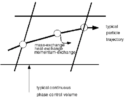
3.2.7 Coupling between the Discrete and Continuous phases ... 27
3.2.8 Momentum exchange ... 27
3.2.9 Heat exchange ... 28
3.2.10 Mass exchange... 28
3.3 Droplet temperature laws ... 29
3.3.1 Inert Heating or Cooling ... 29
3.3.2 Mass transfer during equation 3.47 ... 30
3.3.3 Droplet Boiling ... 31
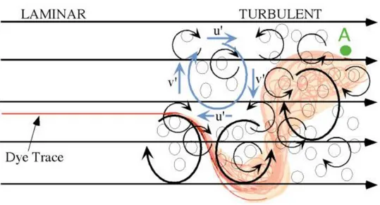
3.4 Turbulence (continuous phase) ... 32
3.4.1 3.2.1 The energy cascade and the Kolmogorov hypothesis ... 33
3.4.2 The Reynolds equation for turbolent motion ... 34
3.4.3 The reynolds Stress ... 35
3.4.4 The 𝜅 − 𝜀 model ... 37
3.4.5 The law of the wall ... 38
3.5 Computational Fluid Dynamics ... 39
3.5.1 Component of a numerical solution method ... 39
3.5.2 Numerical grid ... 40
3.5.3 Convergence criteria ... 42
3.5.4 Boundary conditions ... 43
4 Results and discussion ... 44
4.1 2D test case ... 44
4.1.1 Case settings description ... 44
4.1.2 2D Mesh description and independence ... 45
4.1.3 Droplet injection temperatures (heat description) ... 48
4.1.4 Trap and Escape boundary temperature problems ... 49
4.1.5 Wall-film boundary condition ... 53
4.2 Mesh 3D Desert Tortoise experiment ... 58
4.2.1 3D Mesh description and independence ... 59
4.2.2 Direction of plot ... 61
4.2.3 Elaboration of the experimental data ... 62
4.2.4 Setting used for the detailed description of the cases ... 62
4.3 3D case results and discussions ... 67
4.3.1 Monin-obukhov validation ... 68
4.3.2 3D Case 1 and case 2 ... 69
5 Conclusions ... 79 6 Bibliography ... 81
i
Summary
Introduction
The ammonia is one of the most important product of the chemical industry, in the past the ammonia production was the reference to understand the industrial evolution of a country, in fact the world production of ammonia in 2004 was about 109.000.000 tons. The driving force that promoted the ammonia production was the necessity to produce fertilizers for corps. Due to this bear the necessary to store ammonia in an efficient way. Three methods exist for storing liquid ammonia (Hale, Nitrogen, 1979) (Hale, Nitrogen, 1980):
- Pressure storage at ambient
temperature in spherical or cylindrical pressure vessels having capacities up to about t
- Atmospheric storage at in insulated cylindrical tanks for amounts to about per vessel
- Reduced pressure storage at about 0°C in insulated, usually spherical pressure vessels for quantities up to about 2500 t per sphere.
The first two methods are preferred and is opinion that reduced pressure storage is less attractive.
An area which deserves special attention with respect to safety is the storage of liquid ammonia. In contrast to some other liquefied gases (e.g., LPG, LNG), ammonia is toxic and even a short exposure to concentration of may be fatal. The explosion hazard from air/ammonia mixtures is rather low, as the flammability limits of 15-27% are rather
narrow. The ignition temperature is . Ammonia vapor at the boiling point of has vapor density of ca. of that of ambient air. The important reason why ammonia must be analyzed is its peculiar behavior: the molecular weight of ammonia is 17 g/mol , that is lighter than air 28.9 g/mol. The comparison of the molecular weights yield to anticipate a “light gas” behavior; this is not true due to the temperature field caused by the two-phase release.
Theoretical background
Analyzing the behavior of ammonia subject to a release from a pressurized vessel we have to take into account many aspects. The major factors which influence the amount of material which becomes airbone during an accidental release are the storage pressure and volatility of the material as reflected in its normal boiling point or vapor pressure curve. Releases of pressurized gases usually dissipate rapidly by the energetic mixing associated with high-momentum jet. Releases of pressurized liquids often pose a greater threat because they can form an immediate large air-borne mass of aerosol droplets. The aerosol increases the cloud density both directly and by depressing the cloud temperature by evaporation (as ammonia). Heavier than air clouds tend to disperse less than neutrally buoyant clouds both because they typically flow in the lower wind speeds near the ground, and also because dispersion is suppressed inside a heavy gas cloud.
Liquids stored below their normal boiling point, or as supercooled liquids normally present a lower risk because the discharged liquids form little or no airbone aerosol. Rather they rainout immediately and form a pool of relatively low volatility. However, even high boiling-point materials can form aerosols if discharged from an elevated point, or if they
ii
are stored under pressure with a padding gas. Aerosol formation occurs by mechanical shearing, termed aerodynamic breakup, the foregoing flow behavior shows that the flashing region is a complex problem and the transition between initial super-heated liquid state and the following two-phase jet is not well understood (R.K. Calay, 2007).
The liquid in aerosol form initially has a vapor pressure of one atmosphere, and continues to evaporate as it follows a trajectory along the plume. Typically the droplets cool thereby increasing the temperature driving force. This continues until the temperature driving force reaches an equilibrium so that heat loss by evaporation balances heat gain by conduction and radiation from the surroundings. The vapor pressure of the droplets decreases upon cooling, which reduces the evaporation rate of the aerosol and also that of the pool which forms from rainout or drops reaching the ground.
Rainout from aerosol clouds can form a wetted surface and/or a spreading pool. Rainout lowers the concentration in the cloud, but also tends to prolong the hazardous event by subsequent evaporation. A short discard event is transformed into a long lasting event by rainout and evaporation (Americal institute of chemical engineers , 1999).
Governing equations
The conservation equations for mass, momentum, energy (temperature) and concentration have been used to simulate the process of interest. Dρ Dt = −ρ(∇ ∙ v) ∂ρv ∂t + (∇ ∙ ρ(v ∙ v)) + (∇ ∙ P) − ∑ ρsFs= 0 s ∂ ∂t[ρ (e + 1 2V 2)] + ∂ ∂x[ρu (e + 1 2V 2)] + ∂ ∂y[ρv (e + 1 2V 2)] + ∂ ∂z[ρw (e + 1 2V 2)] = −∂qx ∂x − ∂qy ∂y − ∂qz ∂z + ∂ ∂x(uσxx+ vσxy+ wσxz) + ∂ ∂y(uσyx+ vσyy+ wσyz) + ∂ ∂z(uσzx + vσzy+ wσzz) + ρugx+ ρvgy + ρwgz
With the help of the 𝜅 − 𝜀 model, which is almost universally adopted in the study of dispersion despite its known limitations. The turbulent viscosity was calculated using the Prandtl-Kolmogorov equation. As a function of turbulent kinetic energy, κ, and its dissipation rate, ε, by the closure model defined as follows: 𝜕 𝜕𝑡(𝜌𝑘) + 𝜕 𝜕𝑥𝑗[𝑢𝑗(𝜌𝑘)] = 𝜕 𝜕𝑥𝑗 [(𝜇 +𝜇𝑡 𝜎𝜅 )𝜕𝑘 𝜕𝑥𝑗 ] + 𝐺𝑘 − 𝜌𝜀 ∂ ∂t(ρε) + ∂ ∂xj[uj(ρε)] = ∂ ∂xj [(μ +μt σε ) ∂ε ∂xj ] + C1εε kGk − C2ερ ε2 k
The liquid phase consisting of particle droplets was modeled by a Lagrangian approach. The discrete phase particle trajectories can be computed by integrating the force balance equation. The fluid phase influences the particle via drag, turbulence and momentum transfer. The particle influence the fluid phase through source terms. Mass, momentum as well as energy transfer between the phases were included. For the discrete phase (small droplets of liquid ammonia).
iii
DPM temperature laws
The inert heating or cooling laws (equations and) are applied when the particle temperature is less than the vaporization temperature that have been defined, 𝑇𝑣𝑎𝑝, and after the volatile fraction, 𝑓𝑣,0, of a particle has been consumed.
𝑇𝑃 < 𝑇𝑣𝑎𝑝
𝑚𝑝 ≤ (1 − 𝑓𝑣,0)𝑚𝑝,0
The equation above. is applied until the temperature of the droplet reaches the vaporization temperature.
When using TP < Tvap, DPM uses a simple heat balance to relate the particle temperature, 𝑇𝑝(𝑡), to the convective heat
transfer and the absorption/emission of radiation at the particle surface:
𝑚𝑝𝑐𝑝 𝑑𝑇𝑝
𝑑𝑡 = ℎ𝐴𝑝(𝑇∞− 𝑇𝑝) + 𝜀𝑝𝐴𝑝𝜎(𝜃𝑅 4
− 𝑇𝑝4)
The equation is applied to predict the convective boiling of a discrete phase droplet until the temperature of the droplet has reached the boiling temperature, 𝑇𝑏𝑝, and while the mass of the droplet exceeds the nonvolatile fraction, (1 − 𝑓𝑣,0):
𝑇𝑝 ≥ 𝑇𝑏𝑝
𝑚𝑝 > (1 − 𝑓𝑣,0)𝑚𝑝,0
When the droplet temperature reaches the boiling point, a boiling rate equation is applied: 𝑑(𝑑𝑝) 𝑑𝑡 = 4𝑘∞ 𝜌𝑝𝑐𝑝,∞𝑑𝑝(1 + 0.23√𝑅𝑒𝑑)𝑙𝑛 [1 + 𝑐𝑝,∞(𝑇∞−𝑇𝑝) ℎ𝑓𝑔 ]
Field study setup
The Desert Tortoise field study, was a series of four pressurized liquid ammonia releases made with varying release times and release rates, that was conducted in August and September of 1983 by Lawerence Livermore National Laboratory (LLNL). The test location chosen for the experiments was the Frenchman’s Flat, Nevada, that provided flat terrain with relatively steady and predictable winds.
A pair of tanker trucks were placed on site and the lines leading from each tanker were routed to a common 6-inch diameter spill line. The spill line was extended a sufficient distance cross-wind, such that the tankers and other site equipment would not represent upwind obstacles to the release. The spill line was terminated at an exit plate which reduced the exit diameter to either 3.19 or 3.72 inches. The setup was configured so that the released ammonia would be in the liquid phase when it reached the exit plate.
The field experiment recorded data on flow and temperature from the release, along with meteorological data and video recordings of the release. Concentrations were monitored at distances of 100 and 800 meters from the source.
Once released to the atmosphere, the liquid flashed into a two-phase jet of gaseous ammonia and liquid ammonia drops. Two cross-jet lines of monitors were positioned at 100 meters and 800 meters. Additional monitors were positioned at much greater distances, but failed to collect significant data. Monitors at the 100 meter distance were placed with a horizontal spacing of 15.24 meters. At the 800 meter distance the horizontal spacing was 100 meters. (Christopher G. DesAutels, 2010) (Goldwire, 1985).
iv
2D Test case: mesh description
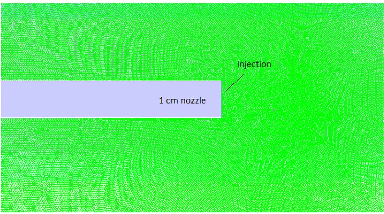
In order to better understand the behavior of the DPM under specific conditions, a 2D mesh has been designed. The mesh is a 3 meters high and a 5 meters long rectangle, with an injection at 1.5 m from the ground. The cells are about 660,000, and are thicken near the droplet release, allowing every simulation to compute 200 droplets from a 1 cm release (Figure 0-1).
Figure 0-1: 2D mesh
The boundary conditions used for this case are: velocity inlet for the inflow, pressure outlet for the outflow, wall for the ground and top, and velocity inlet for the droplets release. 2D mesh validation
When a simulation has to be performed the first step is to check the independence of the results from the mesh size: the cell number can not influence the results. In order to choose the best grid, 3 grids have been designed: 130000 cells grid, 660000 cells grid and a 2700000 cells grid.
The first grid was designed applying a structure function starting from the nozzle (which cell number had been set to 100) and defining the maximum cell size. With this method has been designed the 130000 cells mesh. The 660000 and 2700000 cells mesh were obtained thanks to the “Adapt” option
(Fluent user manual) which sets a node in the middle of the cells, resulting with the quadruplication of the number of cell per every adaption. Figure 0-2and Figure 0-3 show the comparison of the ammonia mole fraction in two directions.
Figure 0-2: Ammonia mole fraction along y axis
Figure 0-3: Ammonia mole fraction along x axis Test case: settings description
With the objective to understand the behavior of the Discrete Phase Model, many simulations were performed emphasizing the sensitivity of the model to the boundary conditions, because was noticed the non physical droplet temperature was reached under some conditions. Tab. 1 shows the
0 1 2 3 0,15 0,2 0,25 0,3 0,35 0,4 0,45 0,5 Distance [m] N H 3 mo le frac ti o n [ -] Mesh Independence 2700000 660000 165000 0 1 2 3 4 5 0,1 0,3 0,5 0,7 0,9 Distance [m] N H 3 mo le frac ti o n [ -] Mesh validation 2700000 660000 165000
v
properties used to describe the mixture template. Tab. 2 shows the properties defined for the fluids description. The properties followed by * are the standard functions in Fluent. The only customizable property is the
piecewise-polynomial describing the
ammonia , due to the improper range of temperature described by the standard function.
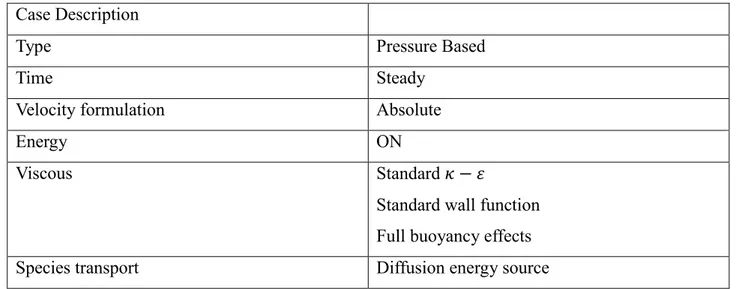
Case description
Type Pressure based
Velocity formulation Absolute
Energy On
Viscous Standard 𝜅 − 𝜀
Standard wall function Full buoyancy effects Species transport Diffusion energy
source
Tab. 1: Mixture properties description
Air Ammonia
Viscosity Constant* Constant*
𝐶𝑝 Piecewise-polynomial* Piecewise-polynomial Thermal coeff. Constant* Constant*
Tab. 2: Fluid property description
Density ( Kg/m3 ) 683 Cp ( J/Kg K ) -5311.9 + 121.71 𝑇 – 0.5051 𝑇2+ 0.0007 𝑇3 Thermal conducivity (W/m K) 0.665 Latent Heat ( J/Kg ) 1368293 Vaporization temperature ( K ) 100
Tab. 3: Drolet functions
The description of the droplets (see Tab. 3) was performed following the DIPPR (Design institute of physical property data) database, with constant parameters, except the saturation vapor pressure which was described with a piecewise linear function. Many aspects were analyzed: Tab. 4
summarizes all the cases and their differences.
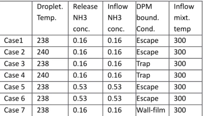
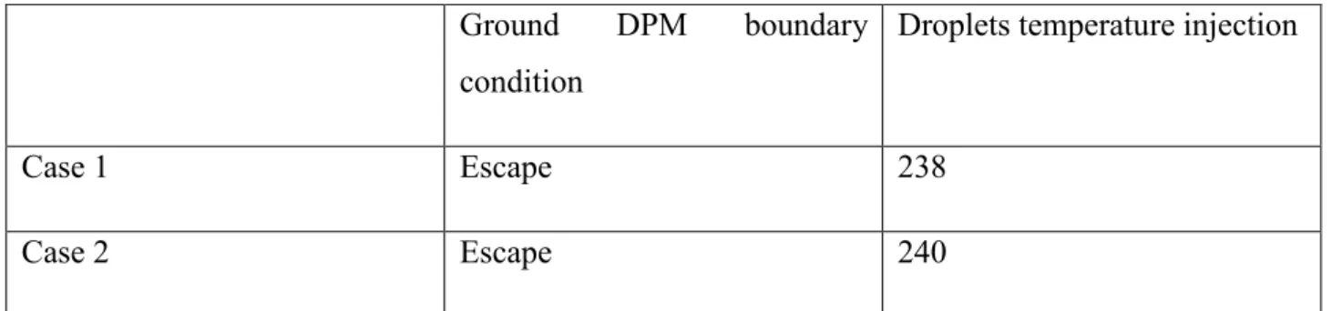
Droplet. Temp. Release NH3 conc. Inflow NH3 conc. DPM bound. Cond. Inflow mixt. temp Case1 238 0.16 0.16 Escape 300 Case 2 240 0.16 0.16 Escape 300 Case 3 238 0.16 0.16 Trap 300 Case 4 240 0.16 0.16 Trap 300 Case 5 238 0.53 0.53 Escape 300 Case 6 238 0.53 0.53 Escape 300 Case 7 238 0.16 0.16 Wall-film 300
Tab. 4: Cases settings
2D Test case: results and discussion
Many issues regarding the minimum temperature reached by the systems were encountered during the simulations. In order to understand the behavior of the DPM was performed a sensitivity analysis.
The comparison of the results between Case 1 and Case 2 led to deeply different results in terms of droplet temperature, despite the only difference refers to the droplet injection
temperature: the minimal droplet
temperature reached in case 1 is below the boiling temperature and is 212,14 K, on the other hand the minimal temperature reached in Case 2 is 239.85 (which is the boiling temperature set for the ammonia). The reason of this lays in the different laws taken into account in the calculations; the equations used do not allow to the droplet to reach a lower temperature then the boiling point. The same conclusion can be reached analyzing the results gained with Case 3 and Case 4, the only difference, compared to the previous, is
vi
the adoption of the Trap boundary condition. In these simulations another aspect must be taken into account: the Trap conditions forces the instantaneous evaporation of the liquid phase as the droplet reaches the boundary. This behave led to inconsistent air temperature (1 K in both cases) and also affected the droplet temperature only in Case 3 (due to the equation applied).
Droplet minimum temperature Air minimum temperature Case 3 183 K 1 K Case 4 239.85 K 1 K
Tab. 5:minimum temperatures
Figure 0-4 Droplet temperature Case 3
Figure 0-5: Air temperature case 3
The only way to quench this shortcoming is to impose the lower limit temperature of the system.
Case 5 and Case 6 were performed in order to check the correspondence of the lower temperature reached with the vaporization pressure: Droplet release temperature 𝑁𝐻3 minimum concentration allowed Droplet minimum temperature Case 1 238 0.16 212 Case 5 238 0.53 226 Case 6 238 0.9 236 Tab. 6
The same results can not be reached with the Trap boundary condition due to the effect of the cooling air. Comparing the results obtained with cases 1, 5 and 6 was proved the respect of the Raoult law in order to describe the equilibrium temperature between the liquid and vapor ammonia phase, moreover, this consistent behavior underlines that the temperature issues analyzed with the previous cases are caused by bug of the Ansys fluent. In Case 7 the wall-film boundary condition was tested. This type of boundary condition requires the switch to a unsteady simulation. In this situation the DPM shows its stochastic behavior.
vii
Figure 0-7:Ammonia mole fraction at time 0.1 and 0.2
Figure 0-8: Droplet Temp at time 0.8 and 0.9 sec
Figure 0-9: Amonia mole fraction at 0.8 and 0.9 sec
Figure 0-10: Droplet Temp at time 1 and 1.2 sec
Figure 0-11: Ammonia mole fraction at time 1 and 1.2 sec As long as the droplet follows its trajectory, the temperature drops according to the heat
balance due to evaporation. From Figure 0-8
to Figure 0-11 is shown the formation of the pool: the droplets still cool down due to evaporation. The simulation stops when the pool widen and starts to escape from the
outflow boundary. The minimum
temperatures reached by the system at every time step are listed below:
From Figure 0-7 to Figure 0-11 the ammonia mole fraction at every time step is shown, as long as the droplet are injected the plume widen. Particular attention must be paid at time 0.9 sec: can be noticed the increase of the ammonia near the ground, this is due to the formation of the pool, which can be seen in Figure 0-8.
3D case settings
Four cases were described in order to reproduce the Desert Tortoise experiment, Case 1 and Case 2 are made with the same general settings of the 2D cases, Case 3 and Case 4 are made with the settings shown in Table 7 and 8:
Air + NH3 mixture
Density Ideal gas
Cp Mixing-Law
Thermal conducivity Mass-weighted mixing law
Viscosity Mass-weighted mixing
law
Mass diffusivity Kinetic – theory Thermal diff. coefficients Kinetic – theory
viii NH3 (l) Property temperature dependence Density ( Kg/m3 ) 683 Cp ( J/Kg K ) -5311.9 + 121.71 𝑇 – 0.5051 𝑇2+ 0.0007 𝑇3 Thermal conducivity (W/m K) 0.665 Latent Heat ( J/Kg ) 1368293 Vaporization temperature ( K ) 100 Boiling Point ( K ) 239.85 Volatile component fraction ( % ) 100 Binary diffusion coefficient ( m2/s ) 3.05e-05 Saturation vapor pressure (Pa) -1E+07 - 196704 𝑇 – 909.48 𝑇2 + 1.4137 𝑇3
Tab. 8:Droplet functions 3D case mesh validation
The domain is 900x200x200 m3 (respectively: lenght, width, height).Only half domain of the Desert Tortoise was modeled in order to save computational effort. So that, the release surface is a half circle with a diameter of 0.53 m at 0.79 m height; it is also used as the injection for the NH3 droplets with the DPM. A 1 meter long solid part is shaped at the release in order to soften the turbulence that would be created just placing a surface, the rest of the domain is empty. The inlet is modeled as a velocity inlet with a user defined function for the description of the velocity field, the outlet is a pressure outlet, the top and the sides are symmetry planes, the ground is a wall with a roughness of 0.03 m. The resolution of the mesh is about 1250000 cells. Figure 0-12 shows the 3D mesh. Figure 0-13 shows a particular of the injection surface.
Figure 0-12: 3D case
Figure 0-13: 3D case injection particular
It can be seen in the particular that the mesh was built with a particular structure: the first 15 meters (from the bottom) has been designed with parallelepiped cells, because the flow was anticipated to be smooth and regular in front of the release. The rest of the domain is made with exagonal cells in order to reduce the number of cells within the domain. In order to validate the results gained with the mesh described a new mesh was obtained thanks to the “adapt” option provided by Fluent ( see a fluent user manual). The result is a mesh with about 10,000,000 cells. The comparison between the two meshes is shown in Figure 0-14: the plot regards the ammonia molar fraction along the x axis. By the comparison of the graphs is possible to assume the independence of the results from the mesh.
ix
Figure 0-14: ammonia molar fraction along x axis Case 1 and Case 2
For these cases the same settings of the 2D test cases have been used. The simulations regard the comparison between a case set up considering the Escape (case 1) boundary condition and the Trap (case 2) boundary condition. The problems regarding the
temperature persist, indeed, the
temperatures are: Droplet temp. [K] Air temp. [K] Rain-out Case 1 159 201 68 % Case 2 1 1 75 %
Tab. 9: minimum temperatures reached by cases The results gained thanks to these two cases led to not accurate results: both the width and the altitude of the plume are not correctly predicted, the plumes generated are too light and too narrow compared with the experimental data. This results force the definition of a new series of cases.
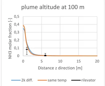
Figure 0-15: Case 1 and2, molar conc ammonia at 100 m along the z xis
Figure 0-16: Case 1 and 2, molar concentration of ammonia at 800 m along the z xis
Case 3 and Case 4
The new settings deeply influenced the results gained: now the plumes are lower and wider, this means that the temperature field is influencing the species field through the density. The most important aspect that changes with the different description of the release is the rain out: see table 10.
0 0,2 0,4 0,6 0,8 1 0 200 400 600 800 N H 3 mola r fra ctio n [ -]
Distance along x axis [m]
Mesh Independence
Mesh 10M cells Mesh 1M cells
0 0,2 0,4 0,6 0,8 0 5 10 15 20 N h 3 mola r fra ctio n [ -]
distance along z axis [m]
Plume altitude at 100 m
escape trap detector
0 0,005 0,01 0,015 0,02 0 50 100 150 200 N h 3 mo lar fra ctio n [ -]
distance along z axis [m]
Plume altitude at 800 m
x Droplet temp release [K] Calculated Rain-out Experim. Rain-out Case 3 240 80 % 40% Case 4 238 30 % 40%
Tab. 10: Calculated and expected rainout
The comparison between the two cases led to appreciable results: as long as we consider section more and more distance from the release the effect of the different description of the source is less and less important; at 100 m the plume in Case 4 is wider and lower then Case 3. See Figure 0-17 and 0-18.
Figure 0-17: Case3 and 4, molar concentration of ammonia at 100m along the z xis
Figure 0-18: Case 3 and 4, molar concentration of ammonia at 800 m along the z xis
The reason that led to an improve of the results must be found in the definition of the properties temperature dependent.
The results gained were checked with the method of the Parabola plot (Hanna & Chang, 1993). The method lays on the calculation of two parameters gained by the ratio between the experimental data and the results gained, these parameters are the geometric mean bias (MG) and the geometric variance (VG) Geometric mean bias (MG) values of 0.5- 2.0 can be thought of as a “factor of two” over predictions and under predictions in the mean respectively. A geometric variance (VG) value of about 1.5 indicates a typical of two scatter between the individual pairs of predicted and observed data. If there is only a mean bias in the predictions and no random scatter is present, then the relation (𝑙𝑛𝑉𝐺) = (𝑙𝑛𝑀𝐺)2, is valid, defining the minimum possible value of VG for a given MG.
0 0,1 0,2 0,3 0,4 0,5 0 5 10 15 20 N H 3 mola r fra ctio n [ -] Distance z direction [m]
plume altitude at 100 m
2k diff. same temp rilevator
0 0,005 0,01 0,015 0,02 0 10 20 30 40 50 N H 3 mola r fra ctio n [ -] Distance z axis [m]
Plume altitude at 800 m
xi
Figure 0-19: case 3 and case 4 parabola plot The parabola plot confirms the supposition mad analyzing the plots: the Cases tend to overestimate the results, Case 4 has a geometric mean higher then 0.5, case 3 has a MG lower then 0.5 this means that case 3 over estimates the results more then 2 times. Case 1 and case 2 led to results so non predictive that result with values of MG bigger then 500.
Conclusions
The purpose of this work is to set up a case able to reproduce the experimental data of the Desert Tortoise experiment. The goal has been reached after the study of the Discrete Phase Model, which is a stochastic model that works in a Lagrangian frame. The results from the 2D test case led to understand the main problem of the model: the laws that describe the physic of the problem are depending of the release temperature.
When droplets, below the boiling point, are injected into the domain their temperature drop can not be limited by the proper description of the condensation and solidification (temperatures reach 1 K), the method to avoid this inconsistence is either to
limit the lower temperature of the system or to describe the condensation process throw a user defined function.
When the droplets above the boiling point are injected into the domain their temperature is no more related, by a heat balance, to the continuous phase but only the mass loss is calculated (that’s why the minimum temperature reached by the droplet is equal to the boiling temperature). Other authors chose this description of the release in order to avoid temperature problems.
An other important aspect that has been taken into analysis is the boundary condition that refers to the DPM the boundary condition analyzed are: Trap, Escape, Wall-film. The Trap boundary condition forces the evaporation of the droplet when it reaches the ground, leading to a temperature drop of the surrounding air (1 K) when a huge rain out is carried out, which is inconsistent. Again, limiting the temperature of the system is the only way to quench this issue.
The Escape boundary condition didn’t led to temperature problems, but the mass loss related to the assumption of this condition do not fit the purpose of this work and have been rejected in the description of the 3D case representative of the Desert Tortoise experiment.
The Wall-film boundary condition is the only one that works only in a time dependent simulation. The advantage of this condition is that takes into account all the aspect of the physic of the droplet when reaching the ground: break, pool formation, evaporation, etc… the eventually condensation over the surface of the droplet is still not taken into account. 0,5 1 1,5 2 2,5 3 0,25 2,5 VG MG
Parabola plot
xii
In order to represent the Desert Tortoise two set of cases have been described: the first set is described with the help of the standard functions set up by Fluent, the second set has been built with the help of the DIIPR data regarding the air and the ammonia, and, where possible, temperature dependent laws have been preferred.
The Cases set up with the less accurate set of settings led to results far from the experimental data in our possess, failing in the prediction of the altitude and the width of the plume. The Introduction of a more accurate set of settings led to a more real-like simulation, which has been analyzed with the Parabola plot method, confirming a
overestimation of the results.
In order to achieve a more realistic description a sentivity analysis should be carried on, leading to the choice of those factors and laws more representative of the case analyzed.
1
1 Introduction
The ammonia is one of the most important product of the chemical industry, in the past the ammonia production was the reference to understand the industrial evolution of a country, in fact the world production of ammonia in 2004 was around 109,000,000 tons. The leading force that promoted the ammonia production was to produce fertilizers for corps. Due to this bear the necessary to store ammonia in an efficient way. Three methods exist for storing liquid ammonia:
1) Pressure storage at ambient temperature in spherical or cylindrical pressure vessels having capacities up to about 1500 t
2) Atmospheric storage at 240 K in insulated cylindrical tanks for amounts to about 50000 t per vessel
3) Reduced pressure storage at about 273 K in insulated, usually spherical pressure vessels for quantities up to about 2500 t per sphere.
The first two methods are preferred and is opinion that reduced pressure storage is less attractive. Analyzing the behavior of ammonia subject to a release from a pressurized vessel we have to take into account many aspect. First we have to consider that the phase released is liquid at the vessel conditions (if we suppose no change phase in the release section set between the stagnation condition and the exit orifice) but at the normal conditions ( T= 1atm, P=101325 Pa) the stable phase is gas. The phase exchange, assisted with the rapid expansion due to the pressurized storage, determine a drop of the temperature which prevents the total evaporation of the liquid phase. Is coarsely possible to divide the zone immediately after the release into two zone to gain a better understanding of the problem. In the first zone the behavior of the compound is mainly determinate by the pressure gradient that sets the momentum at the release and the rapid expansion and evaporation driving the component to the atmospheric pressure and to its minimum temperature, in the second zone the effect of temperature grows leading to evaporation of the liquid phase until reaches the atmospheric temperature. This clarification is important because helps to identify a pseudo-source in which the ammonia is expanded; this theoretical surface will be the source in the CFD calculations. This method is helpful to avoid the description of the distribution of the droplets size that is generated by mechanical friction during the release at the nozzle, so is coarsely possible to define an average droplets size instead of defining the all distribution it is important to underline that the droplet size may have a strong effect on the downstream temperature of the plume.
2
weight of ammonia is 17 Kg/mol, that is lighter than air (28,9 Kg/mol). The comparison of the molecular weights yield to anticipate a “light gas” behavior; this is not true due to the two-phase release: the evaporation of the liquid ammonia cools down the temperature of the stream leading to the condensation of the water vapor determining, taking into account the liquid ammonia itself, an increase of the average density. This leads to a plume that doesn’t lift, typical of the “heavy gas”, and, if the liquid mass flow rate is enough, to the formation of a pool. As long we move downstream the entrainment of air, due to the turbulence, becomes predominant, the average density drops, and the plume becomes comparable first to a “neutral gas” (where the vertical dispersion is determined by the vertical gradient of temperature of the air) then to a light gas (where the vertical dispersion is increased by the density gradient between the ammonia and the air).
An area which deserves special attention with respect to safety is the storage of liquid ammonia. In contrast to some other liquefied gases (e.g., LPG, LNG), ammoniais toxic and even a short explosure to concentration of 2500 ppm may be fatal. The explosion hazard from air/ammonia mixtures is rather low, as the flammability limits of 15-27% are rather narrow. The ignition temperature is 924 K. Ammonia vapor at the boiling point of 240 K has vapour density of ca. 70% of that of ambient air. However, ammonia and air, under certains conditions, can form mixtures which are denser then air, because the mixture is at lower temperature due to evaporization of ammonia. On accidental release the resulting cloud can contain a mist of liquid ammonia, and the density of the cloud may be greater than that of air.
In ammonia production, storage, and handling the main potential health hazard is the toxicity of the product itself. The threshold of perception of ammonia varies from person to person and may also be influenced by atmospheric conditions, values as low as 0.4 – 2 mg/m3 (0.5 – 3 ppm) are reported but 50 ppm may easily detected by everybody. Surveys found concentrations from 9-45 ppm in various plant areas.
Exposure to higher ammonia concentration has the following effects: 50 – 72 ppm does not disturb respiration significantly; 100 ppm irritates the nose and the throat; 200 ppm will cause headache and nausea; 2500 to 4500 ppm may be fatal after short exposure; 5000 ppm and higher causes death by respiratory arrest.
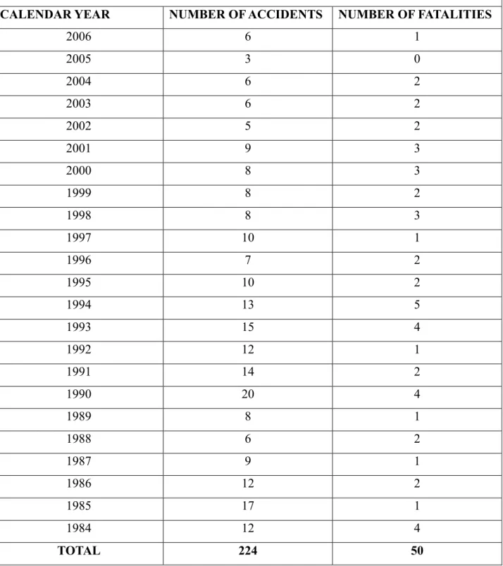
The ammonia is a so common use compound that is impossible to gather all the accidents that occured in history. Anyhow, in order to let the reader to better understand the amount of accident in which ammonia was involved is below purposed (Table 1) a summary of ammonia accidents in the United states to which OSHA (Occupational Safety & Health Administration is part of the United States Department of Labor) responded.
3
OSHA ENFORCEMENT FINDINGS- ACCIDENTS INVOLVING THE RELEASE AMMONIA
CALENDAR YEAR NUMBER OF ACCIDENTS NUMBER OF FATALITIES
2006 6 1 2005 3 0 2004 6 2 2003 6 2 2002 5 2 2001 9 3 2000 8 3 1999 8 2 1998 8 3 1997 10 1 1996 7 2 1995 10 2 1994 13 5 1993 15 4 1992 12 1 1991 14 2 1990 20 4 1989 8 1 1988 6 2 1987 9 1 1986 12 2 1985 17 1 1984 12 4 TOTAL 224 50
4
2 State of the art
2.1 Two phase releases
In many postulated releases from chemical and process plants, the material contained within the plant is ejected through a break as a two-phase jet or cloud which then disperses into the surrounding atmosphere. Estimation of the behavior of released material is necessary for hazard assessment and, for two-phase releases, is obviously more complicated than in the case of single-phase (gas) clouds. Specifically, the liquid phase may be dispersed as small droplets in the flow field, and these droplets evaporate causing changes in the temperature and composition of the surrounding gas. If the surrounding atmosphere is humid, then water vapour may condense on the droplets (which have dropped in temperature due to evaporation) and this gives a further complicating factor in the cloud behaviour. Different approaches, of varying complexity, have previously been taken to predict the behaviour following such releases. The approaches can be divided into three main categories. The first, and simplest, is the `box’ model, in which a buoyancy-driven flow in a wind field is regarded as being transported in a cylindrical shape whilst retaining a self-similar internal concentration field, i.e. the concentration distribution always has the same shape when scaled with the cloud radius and height. The cloud can increase in volume by entrainment of air through its boundaries, and can slump under the action of gravity, spreading outward in a manner analogous to that in the classic dam break problem. This allows solution of a system of `lumped’ ordinary differential equations for species mass, momentum and energy together with an equation of state. Another category of models is known as `similarity’ or `slab’ models, such as that due to Colenbrander, and are really extensions to plumes of the `box’ approach, which applies primarily to puff releases. For transient plumes, a set of partial differential equations involving time and one spatial dimension as interdependent variables is solved. The third main type of model uses a computational fluid dynamics (CFD) approach in which the equations are discretized and solved in all three spatial dimensions.
2.1.1 Theorical background
We focus here on high-momentum atmospheric releases of a liquefied gas or two-phase fluids through a break or a pressure relief system. The release is supposed to originate from a relatively small hole so that continuous, i.e. quasi-steady, conditions at the outlet can be assumed. The cloud is defined as the smallest control volume containing the contaminant. In its first stage, where its initial momentum
5
dominates, the cloud will also be referred to as jet. In most cases involving two-phase releases, the flow is choked at the exit and an external depressurization zone, where the pressure decreases down to the atmospheric pressure, is formed. When the exiting liquid is sufficiently superheated with respect to ambient conditions, it is atomized by violent vaporization (flashing atomization). Otherwise, the liquid or two-phase mixture is disintegrated due to liquid surface instabilities (aerodynamic atomization). Downstream from this region, air entrainment at the perimeter of the cloud becomes important, which causes it to further widen. At least for some distance, the cloud may be dense, i.e. heavier than air, as a result of high molecular weight ,e.g. chlorine. or low temperature and airborne droplets ,e.g. evaporating ammonia (Britter, 1989).
The dispersion of the contaminant in the atmosphere can be described in terms of cloud trajectory and dilution. From an integral point of view, the trajectory is given by a momentum balance on the cloud; the main effects involved are cross-wind, gravity and friction on the ground after touchdown. The dilution is controlled by the rate of air entrained in the cloud. Near the outlet, this is governed by the turbulence generated by the jet itself; it is then controlled by atmospheric turbulence when the jet velocity has decreased close to that of the ambient wind. Moreover, the interaction with a cross-wind induces an enhancement of the entrainment rate. In the case of dense clouds, gravity may also have an effect on air entrainment, related to gravity-induced turbulence as well as suppression of atmospheric turbulence due to stable stratification. In the following, the region of passive dispersion due to atmospheric turbulence only is referred to as the far-field and the upstream region as the near-field.
The dispersion process may be significantly affected by the presence of an aerosol phase. First, two-phase releases can lead to much higher discharge mass flow rates than single-two-phase gas releases (Fauske & Epstein) and, thus, increase the hazard zone distance. Moreover, the jet density may be significantly higher. It can firstly be increased by the mere presence of the liquid phase. However, this is only significant very close to the outlet, where the liquid mass fraction averaged over the jet cross-section is not negligibly small. The aerosol effect on jet density is mainly due to phase change phenomena. When the liquid contaminant evaporates, the jet may significantly cool down and, thus, increase in density. A gas which has a smaller molecular weight than air like ammonia can then behave as a heavy gas. The cooling process may also lead to the condensation of the entrained humidity. If the contaminant is hygroscopic, this can lead to its persistence to significantly larger distances from the outlet. The formation of the aqueous aerosol will cause the mixture to warm up more rapidly and have less density (Wheatley, 1986). Furthermore, a part of the liquid may not remain airborne in the jet and fall to the ground where an evaporating pool could build up; such a pool may also be formed from the jet impingement on a surface. This so-called rainout could induce a drastic reduction of the
6
downstream contaminant concentration but increases the danger close to the source as well as the duration of the dispersion. Besides, it may lead to soil contamination. Finally, the presence of the aerosol also affects the turbulent structure of the jet and, therefore, the air entrainment, the direction of influence (enhancement or suppression). depending on the particle size.
2.2 TWO PHASE DISPERSION MODELS
The dispersion models which take into account the presence of an aerosol phase have appeared only recently ( in the last twenty years) in the literature. They are either integral or multidimensional models. Integral models are obtained by integrating the balance equations for mass, momentum, energy and species over the cloud cross-section. The lateral variations of the local variables, such as velocity, concentration and temperature, can be obtained by introducing lateral profiles in the integrated balance equations. If these profiles are flat ‘top-hat’ profiles., the model reduces to the so-called ‘box’ model. Non uniform profiles, which are supposed to be geometrically similar after a zone of flow establishment, can also be adopted. In multidimensional models, the local time-averaged equations of mass, momentum, energy and species are locally solved in the whole space. Unlike the integral models where turbulent diffusion is implicitly given through the profile shape function, closure must be provided for turbulent stresses.
Because of the high variety of possible situations to be considered in hazard assessment, but which cannot or have not been covered by experiments, the dispersion models are often extrapolated beyond the range where they have been validated. The need for physically-based models is, therefore, very important to increase the reliability of this extrapolation. Moreover, due to the frequent need to study a large number of scenarios, a compromise between model detail and computing time/cost is often required. These conditions are best fulfilled by one-dimensional _integral or box. models, which can be in most cases helpful. However, in some situations associated with obstructed terrain, multidimensional models could be recommended, as it is shown, e.g., (Wurtz, Bartzis, & Venetsanos). They are however complex, costly to run and often faced with numerical difficulties, and require a high degree of expertise.
In the following description, every necessary jet property at the outlet, such as the mass flow rate, is supposed to be known. However, within a short distance just downstream from the outlet, the flow can experience drastic changes which must be considered for subsequent dispersion calculations. The physical phenomena taking place in this region comprise (i). flashing if the liquid is sufficiently pressurized, (ii). Gas expansion when the flow is choked and (iii). liquid fragmentation. The corresponding quantities to be determined as initial conditions for subsequent dispersion are the flash
7
fraction, the jet mean temperature, velocity and diameter, and the drop size. Due to its relatively short length, a global and simplified modelling approach is normally adopted in this region, also in the case of multidimensional models. Therefore, these initial conditions are first described, followed by the description of the integral and multidimensional dispersion models.
2.2.1 Flashing
Flashing occurs when the liquid is sufficiently superheated at the outlet (with respect to atmospheric conditions). and corresponds to the violent boiling of the jet. The vapor quality after flashing, or flash fraction, is most often determined in the models by assuming isenthalpic depressurization of the mixture between the outlet and the plane downstream over which thermodynamic equilibrium at ambient pressure is attained, i.e., any transfer with the surroundings as well as the kinetic energy change are neglected; the temperature reached is the saturation temperature at atmospheric conditions. It should be noted that this calculation is applied in the models as soon as the liquid is superheated. In this approach, the neglect of the kinetic energy change seems to be justified due to the large contribution of the heat of vaporization in the energy equation (Wheatley, 1986). However, a more general expression, where this assumption is relaxed, is recommended by (Britter R. E.). Adiabatic and frictionless conditions as well as the absence of air entrainment are reasonable approximations provided that the distance up to the point where thermodynamic equilibrium at atmospheric pressure is reached, is short enough. Atmospheric pressure is in general attained after a flow length of about two orifice diameters and the flashing phenomenon is observed to occur very fast so that these assumptions should be met in practice. When the liquid is not sufficiently superheated for flashing atomization to occur, the flow path before thermodynamic equilibrium is restored, could be greater. However, the degree of non-equilibrium being low in this case, the above assumptions should still be acceptable.
2.2.2 Expansion
When the flow is choked at the outlet, the gas phase expands to ambient pressure within a downstream distance of about two orifice diameters. This causes a strong acceleration of the two-phase mixture and usually an increase of the jet diameter. In the models, the velocity and diameter of the jet at the end of the expansion zone are given by the momentum and mass balance, respectively, integrated over a control volume extending from the outlet to the plane where atmospheric pressure is first reached. It is assumed that no air is entrained in this region. An alternative model based on isentropic expansion has been proposed by Woodward (Woodward, 1992). This led to substantially different results.
8
This control volume approach, which cannot provide the variations within the expansion zone, appears to be suitable in view of its short length. The absence of air entrainment is also justified by the strong lateral expansion. Because of the lack of experimental data, the alternative predictions obtained by using the model of Woodward could not yet be validated. Finally, it should be noted that the flow speed can be increased by a factor as high as 10 in this region, which has important consequences on the downstream dispersion (Wheatley, 1986).
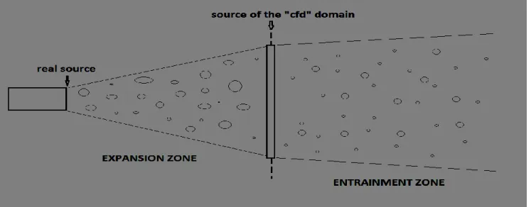
2.2.3 Expansion zone: source of the CFD domain
Flashing is violent break-up of the pressurized liquid into small droplets which occurs when a super-heated liquid comes in contact with ambient conditions (atmospheric temperature and pressure) at a point of a leak. The combination of hydrodynamic instabilities and thermal non-equilibrium conditions lead to flashing. The meta-stable liquid can only come to its equilibrium condition by releasing its super-heat through evaporation which consists of boiling and vaporizing of the droplets as they disperse in ambient air and provide an explosive characteristic to the process. Fig. 2-1. shows a schematic representation of a flashing liquid jet issuing from a circular nozzle. The flashing location depends upon the geometry of the leak, initial conditions and the liquid properties. In Fig. 2-1 flashing is shown occurring outside the nozzle but flashing may begin inside the pipe or vessel. It has been observed experimentally that the ‘expansion’ region is made up of large droplets and liquid ligaments moving with increasing velocity. The velocity starts to decrease in the entrainment region due to mixing with ambient air as jet propagates. The axial temperature keeps decreasing well below the boiling temperature at ambient pressure further downstream and reaches its minimum as droplets evaporate. Beyond this point the temperature rises to ambient value. The droplet sizes and velocity mean values also decrease due to evaporation in the entrainment region. The radial variation of droplet size, temperature and velocity at different locations along the axis of the jet shows approximately Gaussian distribution. The foregoing flow behavior shows that the flashing region is a complex problem and the transition between initial superheated liquid state and the following two-phase jet is not well understood. However, varying combinations of boiling and evaporation processes are present alongside severe mechanical break-up of droplets and turbulent mixing between the jet constituents and between these and the ambient air.
9
Fig. 2-1: Schematic rapresentation of the expansion zone
When the flow is choked at the outlet, the gas phase expands to ambient pressure within a downstream distance of about two orifice diameters. This causes a strong acceleration of the two-phase mixture and usually an increase of the jet diameter. In the models, the velocity and diameter of the jet at the end of the expansion zone are given by the momentum and mass balance, respectively, integrated over a control volume extending from the outlet to the plane where atmospheric pressure is first reached. It is assumed that no air is entrained in this region. An alternative model based on isentropic expansion has been proposed by (Woodward., 1992). This lead to substantially different results. This control volume approach, which cannot provide the variations within the expansion zone, appears to be suitable in view of its short length. The absence of air entrainment is also justified by the strong lateral expansion. Because of the lack of experimental data, the alternative predictions obtained by using the model of Woodward could not yet be validated. Finally, it should be noted that the flow speed can be increased by a factor as high as 10 in this region, which has important consequences on the downstream dispersion (Wheatley, 1986)
2.2.4 Drop Size
The models incorporating fluid dynamic and thermodynamic non-equilibrium phenomena, like rainout or droplet evaporation, require sub models for the determination of the initial drop size. There are basically two main mechanisms for atomization: flashing and aerodynamic atomization. With flashing atomization, the fragmentation results from the violent boiling and bursting of bubbles in the superheated liquid, whereas aerodynamic atomization is the result of instabilities at the liquid surface. Most authors do not use any specific criterion to determine which mechanism dominates and
10
deliberately select one of them. Nevertheless, (Ianello, Rothe, & Wallis, 1989) use a mechanistic criterion based on a critical superheat corresponding to the activation of a nucleation site. It requires, however, the specification of a characteristic nucleation site radius for which reliable predictive relations are not available consider that the actual regime is the one which predicts the smallest stable drop size. A comparison of these criteria with available empirical relations relying on experiments with low velocity jets (Brown, 1962) could be fruitful. In any case, more studies on this transition region where both fragmentation regimes may play a role are clearly needed. In the case of aerodynamic fragmentation, the maximum stable drop size is usually given by a critical Weber number, which represents the ratio of inertia over surface tensionforces:
𝑊𝑒𝑚𝑎𝑥 = ∆𝑈2𝜌𝑔𝑑𝑚𝑎𝑥/𝜎 ( 2.1)
where 𝜎 is the (static) surface tension of the liquid, 𝜌𝑔 the gas density,𝑑𝑚𝑎𝑥 the maximum stable droplet diameter and ∆𝑈 the mean relative velocity between both phases. In the models, ∆𝑈 is calculated as the jet mean absolute velocity at the end of the expansion zone in the case of choked flow conditions and the subcritical outlet velocity otherwise. This implies that interfacial stress occurs at contact with the surrounding still air, which is justified in the case of a single-phase liquid jet. However, if a two-phase choked flow were to occur at the outlet, the fragmentation will be induced by the shear stress between the liquid and the accelerating released gas and, thus, a more appropriate relative velocity should be based on the difference between the jet velocity at the end of the expansion zone _representative of the gas velocity. and the exit velocity (representative of the liquid velocity). Moreover, the number 𝑊𝑒𝑚𝑎𝑥 default values ranging are between 17 and 44, with a possible dependence on stagnation pressure (or exit velocity), have been tested by (Muralidhard, 1995); their best prediction for the liquid capture on the ground was obtained with the value of 𝑊𝑒𝑚𝑎𝑥 depending on pressure. The experimental observations provide maximum Weber values between 5 and 20 for low-viscosity liquids, with the most commonly used value being 12. The value of 20 can be deduced from a balance on the drop between drag and surface tension forces with a drag coefficient of 0.4, which is an acceptable approximation for a rigid sphere in the turbulent regime (𝑊𝑒𝑚𝑎𝑥 = ∆𝑈 𝑑𝑚𝑎𝑥/𝜇𝑔between 500 and 2𝐸5) as long as the relative velocity is small enough compared to the speed of sound. This is an upper limit for the maximum stable droplet diameter 𝑑𝑚𝑎𝑥 since in reality the particle is deformed and experiences a higher drag during the fragmentation process.
For the flashing atomization, (Ianello, Rothe, & Wallis, 1989) propose a mechanistic model based on a Weber number where the characteristic relative velocity ∆𝑈 is composed of two components, in the axial and radial direction, respectively. The axial component is due to the vapour acceleration in the expansion zone; the relative velocity is taken as the difference between the jet velocities at the end
11
and at the beginning of this zone. The radial component comes from the momentum transfer caused by the rapidly growing bubbles; it is given by the maximum bubble expansion velocity. On the other hand, (Woodward, 1992) have established a correlation for the maximum stable diameter to match rainout experimental data. As indicated by the authors, this relation may not necessarily agree with values measured independently because of incompleteness in some other parts of the dispersion model. Among the relations they considered, the one depending on a so-called ‘partial expansion energy’, which is a measure of the superheat, gave the best results. Moreover, some authors adopt constant default values for the drop size based on experimental results. They usually range between 10 and 100 μm (Pattison & Martini). Moreover, it should be noted that if flashing occurs upstream from the orifice (e.g. in a long pipe), the different flow regimes at the exit could lead to specific fragmentation processes, as shown by the drop size data obtained for the aerodynamic fragmentation of a dispersed-annular flow regime.
Regarding the assumed drop size distribution, every model considers a unique equivalent size except (Ianello, Rothe, & Wallis, 1989) who adopt a log-normal distribution and (Pereira & Chen) who use two size classes. The assumption of one-size droplets is obviously contrary to observations but simplifies the matter. A sensitivity analysis regarding this assumption should, however, be performed. Finally, other authors have shown (Kukkoken, 1993), due to compensating effects, the droplet evaporation rate does not strongly depend on the initial drop size below 100 mm. On the other hand, the results of other authors show (Muralidhard, 1995) that the rainout fraction is very sensitive to the initial drop size.
2.2.5 Integral model
Integral models can either deal with both the near-field and far-field or consider the near-field only. In the latter case, they are regarded as source term for a far-field dispersion model. However, they are similar in principle Some of these models can handle ground-level clouds, i.e., clouds in contact with the ground.
The models are all based on the balance equations for mass, momentum, energy and species, integrated over the jet cross-section; they mainly differ by the adopted closure relations. A common frame based on the mixture balance equations is first proposed to enable a comparison between the models. Then, the closure relations, or sub models, are described.
12
The enthalpy of the jet (mean or centreline value). is given by the two-phase mixture enthalpy balance equation. However, additional relationships are necessary to determine how the overall enthalpy change affects the jet composition and temperature. The jet is a mixture of the released material (liquid and/or vapour)., dry air and, for all considered models but the one of Woodward et al., ambient humidity (liquid and or vapour). Most often, the overall mixture enthalpy is expressed as a function of the enthalpies of the jet components by assuming that the mixture is in thermodynamic equilibrium. Gas and vapour are supposed to behave as an ideal gas. The partial pressures of the released material and the water are usually supposed to be given by their respective vapour pressure at the jet temperature (ideal mixture). The mass and enthalpy equation are separately written for the liquid and gas phases. When ambient humidity condensation is considered, the liquid water is either included in the liquid phase leading to binary droplets or added in the gas phase to form a fog. Heat and mass transfer coefficients are introduced for transfers at the drop surface so that drops and gas or fog can adopt different temperatures.
Kukkonen et al. checked the homogeneous equilibrium model predictions with those of a non-equilibrium approach (different velocities and temperatures for the droplets and the surrounding gas) in the case of two-phase ammonia cloud dispersion in dry and moist air. They concluded that the homogeneous equilibrium approximation seems to be adequate for droplet sizes lower than 100 μm. However, it is noted that this conclusion is only valid as far as the vaporization rate is concerned and may not apply to rainout. It may also not be valid for cases where entrainment is fast, as in the high momentum region of a jet. Moreover, Kukkonen et al. tested the effect of an introduction of ammonia/water interaction in the phase equilibrium. The assumption of non-ideal behaviour of the mixture lowered the volatility of the liquid phase, but exhibited no significant influence on the average temperature. It had, however, the effect of maintaining a low contaminant concentration much further downstream from the source. These authors also performed calculations with the assumption of zero and 100% ambient relative humidity. The difference in temperature could in some part of the dispersion reach 20 K. Similar calculations with Wheatley’s model in the case of ammonia with zero and 100% ambient relative humidity have been also performe. The difference in the jet density and concentration for these extremes was less than 10%. However, the results were restricted to the near-field where gravity effects were not considered significant.
2.2.7 Rainout
As explained by (Wheatley, 1986), provided that the drops are large enough, they are affected by gravity to a greater extent than the surrounding gas. The drops do not remain the same size during
13
their motion but steadily evaporate as the surrounding vapour is diluted by air. From the spectrum of drop sizes formed initially, some drops may be large enough that they fall out of the jet rapidly with no appreciable vaporization, while others may be small enough that they evaporate before reaching the ground. The quantity of rainout is a very important item for dispersion calculations. The description of this complex phenomenon is, however, circumvented by most modelers by assuming that the drops are sufficiently small to remain airborne until complete evaporation. Wheatley has devised a simple criterion for the absence of rainout, leaving aside the problem of what to do otherwise. From the maximum stable drop size in the initial section, the maximum gravitational settling velocity can be found from a force balance. By taking the drop axial velocity equal to the mean initial jet velocity (after the expansion zone), a bound for the initial drop trajectories can be defined. If it subtends a sufficiently small angle with the jet axis (taking it to be horizontal), this implies that rainout can be ignored. Other authors (Ianello, Rothe, & Wallis, 1989) extended this approach by applying the above criterion to the whole spectrum of drop sizes. This enables the fraction of liquid which rains out to be calculated. A more sophisticated approach has been proposed by (Woodward, 1992). The aerosol consists of single-sized spherical droplets. The local droplet diameter and trajectory is obtained by solving the balance equations on the drop for mass, energy and momentum in the vertical direction, simultaneously with the gas jet mean quantities. The horizontal drop velocity is set equal to the horizontal component of the local velocity in the jet, although in a previous version slip velocity was allowed for in the horizontal direction. Rainout occurs when the drop hits the ground. An other author (Muralidhard, 1995) proposed another simple criterion. The liquid phase is supposed to be well mixed within the jet. Rainout is considered to occur when the jet centreline hits the ground (the liquid phase due to ambient humidity condensation is however supposed to remain airborne in the jet). In accordance with the no-slip assumption made in the models, the drop inertia in the axial direction is not taken into account. Consequently, a relatively large drop which is not predicted to rainout according to Wheatley’s approach, or which will fall out at a certain distance as predicted by Woodward’s model, may eventually rainout further downstream.
Transition criteria
Generally, for some specific conditions, the model application range is exceeded or some model relationships must be modified. These conditions correspond to physical transitions for which criteria must be provided. First, a transition between elevated and ground-level clouds must be specified. This simply occurs when the lower boundary of the jet reaches the ground. Moreover, for models which apply only in the region dominated by the initial jet momentum where gravity as well as atmospheric turbulence have no significant effect, transitions towards these regimes must be given. Must be
14
adopted the following criteria to determine when the dispersion is not dominated by the initial momentum any more:
𝑢𝑚⁄𝑢𝑎 ≤ 0.8 Pasive dispersion important
𝑅𝑖 = | 𝜌𝑚− 𝜌𝑎|𝑔𝐷 𝜌⁄ 𝑚𝑢𝑚2 ≥ 0.1 Buoyancy effects important
where D is the jet cross-section diameter and Ri the Richardson number of the jet which represents the ratio of jet buoyancy over jet inertia. Equivalent criteria are mentioned by the other authors when needed.
2.2.8 Multidimensional models
The two-phase multidimensional dispersion models that we consider subsequently are the one of Wu¨rtz et al., Garcia and Crespo, Vandroux-Koenig and Berthoud, Pereira and Chen.
Wurtz et al.’s model
This three-dimensional model includes the mixture mass, momentum and energy balance equations as well as the mass balance equation for the contaminant component. The mixture is composed of the contaminant (liquid and/or) gas. and the ambient gas (no humidity condensation is considered). Thermodynamical equilibrium is assumed, i.e. all the components share locally the same temperature and pressure. The two-phase mixture is supposed to behave ideally, i.e. Raoult’s law is used for the calculation of the partial pressures. A single-phase turbulence model, based on the eddy diffusivity concept, is adopted and modified to take into account anisotropy effects. A vertical slip velocity is allowed for between the liquid and gas phase. Special attention was paid on the model’s ability to handle complex terrain. In particular, liquid deposition on solid surfaces is taken into account. Remarks already made regarding the assumption of thermodynamic equilibrium in the integral models also apply here. The first validation tests performed by the authors have shown the better performance of this model against a 1-D model when obstacles are present.
Garcia and Crespo’s model
This three-dimensional model contains the mixture mass and momentum balance equations as well as the mass balance equation for the contaminant component w48x. The total enthalpy is taken proportional to the contaminant mass fraction. The treatment of the thermodynamics as well as the composition of the mixture are similar to Wurtz et al.’s model. The relative mean velocity between the phases is neglected. The classical
15
Vandroux-Koenig and Berthoud’s model
This model is devoted to the prediction of the near-field dispersion of liquefied propane (Vandroux-Koening, 1997). It is a Eulerian–Eulerian two-fluid model which considers three components: propane (liquid and vapour), dry air and water (liquid and vapour). The condensed water is included in the gas phase to form a homogeneous fog mixture. Balance equations are written for the mass of each constituent, for the momentum of the gas mixture and of the propane droplets, and for the gas mixture energy. The temperature of the propane droplets is supposed to be uniform, equal to the saturation temperature at atmospheric pressure, so that no energy balance equation is needed for the liquid phase. To close the system of equations, a single-phase turbulence model based on the Prandtl’s mixing length theory is introduced for the gas phase. For interfacial transfers, a constant droplet diameter is assumed throughout the calculation. The momentum and heat interfacial transfer terms are calculated from a drag and a heat transfer coefficient, respectively, for rigid spheres. The mass transfer is modelled by assuming that the heat transferred from the gas phase to the droplets completely contributes to vapour production.
According to the authors, the propane droplets are predicted to persist much further downstream than experimentally observed. Several possible causes were investigated for this underestimation of droplet evaporation. Neither the assumption of a constant diameter nor the fact that no initial radial velocity was taken into account could explain this underevaluation. On the other hand, the assumption of a uniform temperature in the droplet or the inadequacy of the turbulence model (the droplets may in reality disperse more than the gas phase) have been proposed as possible explanations. One important assumption which could strongly hamper evaporation and which was not yet discussed, is to take the droplet temperature equal to the saturation temperature at ambient pressure instead of the one corresponding to the vapour partial pressure at the surface (lower due to the dilution of the contaminant vapour). This assumption contradicts the experimental observation that liquid temperature can decrease below the normal boiling point. More parametric studies as well as the comparison of the prediction with the results of controlled laboratory experiments adapted to the validation of the uncertain aspects of the model are required to solve these inconsistencies.
Pereira and Chen’s model
This Eulerian–Lagrangian model is also devoted to the near-field dispersion of liquefied propane; the single-phase version developed for the far-field dispersion is not considered here. It is constituted of a Eulerian description of the mixture phase composed of air and propane vapour (no humidity is taken into account). having the same velocity and temperature but different volume fractions, and a