Wind Tunnel Analysis of an Automotive Wheel and Comparison with Numerical Simulations

SCHOOL OF

ENGINEERING AND ARCHITECTURE

Forlí Campus

-Master’s Degree in Aerospace Engineering

class LM20

GRADUATION THESIS:

in Experimental methods in aerodynamics

Wind Tunnel Analysis of an Automotive Wheel and Comparison with

Numerical Simulations

Candidate :

Riccardo Barberini

Supervisor :

Prof. Gabriele Bellani

Abstract 11

1 Introduction 13

2 Theoretical background 15

2.1 The equations . . . 15

2.2 The boundary layer . . . 16

2.3 The vortex shedding . . . 17

2.4 Aerodynamic of a wheel . . . 23

2.5 Matematical methods . . . 25

2.5.1 Statistical moments . . . 25

2.5.2 The Fourier transform . . . 26

2.5.3 The Welch’s method . . . 28

3 Tools and facilities 31 3.1 The wind tunnel . . . 31

3.2 The Pitot probe . . . 34

3.3 The hot-wire . . . 36 4 Experimental set up 41 4.1 The cylinder . . . 41 4.2 The wheel . . . 43 5 Results 47 5.1 The cylinder . . . 47 5.1.1 Wake features . . . 47 5.1.2 Spectral analysis . . . 48 5.2 The wheel . . . 52 5.2.1 Wake features . . . 52

5.2.2 Extimation of the drag force . . . 57

5.2.3 Spectral analysis and comparison with CFD . . . 57

6 Conclusions 61

2.1 Hermann Schlichting [3]Cd-Re graph. It can be seen how the presence of a laminar boundary layer

leads to a lower drag coefficient (in this case it is considered only the skin friction not the effect of 3D) 17 2.2 Ben L. Clapperton and Peter W. Bearman [4]. Dependence of the drag coefficient to the Reynlods

number. The postion of the plateau depends on the surface roughness of the cylinder. . . . 19 2.3 A.E.Perry, M.S.Chong and T.T.Lim[7]. Behaviour of the flow for different ranges of Reynlods number.

The stable condition holds until Re 40 then the vortex shedding occurs. The vortex shedding then disappears when the Reynolds number lies in the critical region.) . . . . 20 2.4 Uwe Fey, Michael König, and Helmut Eckelmann 1998[8]. Strouhal Reynolds relationship. On the x

axis the Reynlods number is represented as 1 √

𝑅𝑒 so higher value of the Reynlods are at the left of the

graph. The maximum value is reached for a Reynolds near to 1300) . . . . 21 2.5 S.J. Price, D.Sumner.[9] Representation of the experiment conducted by Price in 2002 evaluating the

behaviour of the vortex shedding at different height form the wall . . . . 22 2.6 Fackrell [10] Differences between Cp value of stationary wheel and rotating. It is interesting to see that

the lower peaks are obtained for the stationary case while the higher one for the rotating case. . . . . 23 2.7 Fackrell [10]. Comparison of wake dimension between rotating and stationary wheel at different

dis-tance form the wheel istelf. . . . 24 2.8 Robin Knowles, Alistair Saddington [11]Difference between parallel and cambered wheels. The

pres-ence of a bigger vortex is felt in the cambered configuration, leading to have a greater resistance. . . . 25 2.9 Representation of the most famous statistical moments. . . . 26 2.10 G. D. Bergland [12]Computational cost comparison between direct calculation of DFT and calculation

of DFT using FFT. In the x-axis is represented the number of elements inside the Fourier transform, in the y-axis the number of operations required. . . . 27 2.11 G. D. Bergland[12] Example of how leakage effect occurs. The moltiplication of the sampled signal

with the rectangular data window is the cause of this effect. . . . 28 3.1 Main features of the wind tunnel used for this study. One wall of the test section is made of plexiglass in

order to be able to see what is happening inside, in the opposite wall there is a rounded window from which is possible change the set up inside the test section. The image of the inlet shows the presence of screens and honeycombs, that guarantee the creation of a laminar and organized flow. Being a suction open loop wind tunnel, the fan is installed at the exit of the diffuser as shows the last image.. . . . 32 3.2 Velocity tendency of the flow inside the wind tunnel for different values of velocity. It can be seen that

the variation of velocity is of the order of 10−_{7, thus can be considered negligible. . . . 33} 5

3.3 B.J.McKeon, J.Li [15]Two type of Pitot total port interference: velocity gradient and wall interference.

In the first case the flow particle shift down, so the velocity read is higher than the real one, the opposite happens in the second case. . . . 35 3.4 G.Bellani, A.Talamelli, Lecture notes [16]. Sketch of the static port in a Pitot probe. There exist lot of

variable that can interfere with the reading of the signal. It is very important to understand how the error can be reduced. . . . 36 3.5 Hot wire calibration curve obtained interpolating a 4th polynomial curve. . . . 37 3.6 G.Bellani, A.Talamelli, Lecture notes [16].Relation between Nu and Re. At very low Reynolds number

the relation is dependent on the Grashof number. . . . 38 3.7 G.Bellani, A.Talamelli, Lecture notes [16]. Directional sensitivity of the hot wire anemometer. The yaw

and pitch angle are the ones that can affect the reading of the signal. . . . 39 3.8 The shortening probe it is necessary to evaluate the value of the resistance of the Wheaston bridge and

the cable. Once the hot wire is installed in order to compute the value of the resistance of the sensor it must be subtract the value of the new value of the resistance (Wheaston bridge+cable+HW) to the value previosly calculated. . . . 40 4.1 Close up of the hot wire installed on the traverse system. . . . 41 4.2 Cylinder set up. Here it is shown the cylinder in exam having a diameter of 8cm and length of 58cm.

On the back it is present the hot wire anemometer installed on the traverse system. . . . 42 4.3 Scheme of acquisition points for the study of the cylinder. . . . 42 4.4 The three different types of wheel studied. On the lest there is the wheel with the sharp shoulder, in the

centre the one with edges at 45 degrees and on the right the one with rounded shoulder. . . . 43 4.5 Example of installation of the wheel on the ground. Thanks to the eyelet the wheel can be moved back

and forth in order to evaluate the wake at different positions. Before every acquisition the eyelet is covered by a layer of tape in order to do no permit the air to flow under the ground. . . . 44 4.6 Close up of the strips. When the flow is attached the stripes are steady and directed as the longitudinal

axis of the ground. If the flow separates on the leading edge the strips will move chaotically. . . . 45 4.7 Installation of the traverse system on the wind tunnel. By moving the traverse back and forth and

inclining it with respect the horizontal plane it is possible to cover all the points of a given plane. . . . 45 4.8 Scheme of acquisition points for the study of the wheel wake. . . . 46

5.1 On the left is represented the standard deviation value in the different acquisition points. In the centre

it shown the skewness value of the different acquisition points. On the right it is shown the wake profile of the cylinder with D=0.8m, V=10 m/s evaluated in x/D=1.1. . . . 47 5.2 Comparison of the results of the wake velocity profile behind a cylinder in x/D=1.1 between the actual

data and the one obtained by Ong and Wallace[18] . . . . 48 5.3 Standard deviation, skewness and mean profile of the cylinder evaluated at x/D=8.8 with a velocity

equals to 10 m/s. It can be seen that there is no more the relation between the maximum value of the standard deviation and the highest gradient. The skewness relation still holds true. . . . 48

5.4 Figure a shows the frequency spectrum in function of the shedding frequency, obtained through the

Welch’s method. Figure b shows the frequency spectrum in function of the shedding frequency, obtained through the FFT. The overshoot is much more visible in this case. The Welch’s method reduces this effect by the usage of the windowing. . . . 49 5.5 Some examples of the velocity spectrum. In this case are reported four velocities:1.07;4;7;10 m/s. In

each plot are present four spectra depending on the position of the hot wire. As it might be expected the peaks translates to the right as the velocity increases. Furthermore the second harmonic is more relevant in the case of y/D closer to the wake centre line. . . . 50 5.6 Relationship between frequency and velocity. As expected from the theory it is a linear relationship

proportional to the Strohual number and the diameter. The Strouhal obtained is 0.197. . . . 51 5.7 Voltage and frequency relationship. For each voltage it is extracted the frequency in which it is present

the highest peak. . . . 51 5.8 Comparison between the two calibration curves. The one obtained in the non convential way it diverges

a little from the standard one only at the higher velocities . . . . 51 5.9 Velocity contour of the wake with different types of wheels. In the case (a) the wake is high as the wheel

generating an higher resistance. In (b) the shape is completely different from the previous one and the presence of two big vortices can be seen. In (c) the shape is similar to the one with 45 degrees. The main difference is on the top region of the wake where it seems to be more compact and organized. The lower peaks on the right can be due to a wrong positioning of the hot wire . . . . 53 5.10 Evolution of the wake in the case of the wheel with 45 degrees shoulder. As the distance increases the

wake enlarges and becomes flatter. . . . 54 5.11 Evaluation of the wake in the case of the wheel with rounded shoulder. The behaviour is very similar to

the one obtained in the previous case, where the wake becomes flatter and larger as the distance increases. 54

5.12 Wake of cambered round shoulder wheel at two different distances. On the left z/D=2.25 one the rigth

z/D=3.85. The camber angle has been set to -3.5 . . . . 55 5.13 Wake of rounded shoulder wheel with a camber angle equalo to -3.5° and a toe angle equalo to -0.5°

at two different distances. On the left z/D=2.25 one the rigth z/D=3.85. . . . 55 5.14 Comparison of wake velocity contour between cambered and not cambered wheel in z/D=3.85. It can

be seen a little asymmetry in the case of cambered wheel. . . . 56 5.15 Comparison of wake velocity contour between -0.5° of toe and 0° of toe in z/D=3.85. In this case the

difference is very small. The wake profile in the case of a toe angle different from zero is larger on the left side rather than in the case of no toe angle. . . . 56 5.16 Comparison of the results between experimental (a) and CFD (b) in z/D=1.45. Some similar features

can be seen: the two symmetrical vertices located close to half wheel heigth;a region of faster velocity present at the lower center of the wheel; a circular region of lower velocity over the two vertices. . . . 58 5.17 Comparison of the results between experimental (a) and CFD (b) in z/D=2.25. In both cases there is

no more the presence of the vertices, the wake is more relaxed and it starts to enlarge. . . . 58 5.18 Spectral analysis computed at wake center in different y/D. The location where the peaks are more

relevant is in y/D=0.48, as y/D decreases the spectrum becomes flatter and more noisy. . . . 59 5.19 Spectral analysis computed at y/D=0.5 at different values of x/W. It can be clearly seen the presence of

5.20 Spectral analysis evaluated at y/D=0.5 and x/W=0. The peaks are inside the intervals previously

2.1 Resuming table of different behaviour of Strouhal number depending on the Reynolds number range. . 22 3.1 Value of standard deviation for each velocity. For all the velocities the value of the standard deviation

is very small, this is another indicator of the good quality of the flow. . . . 33 3.2 Evaluation of the velocity inside the test section of the wind tunnel in two different points. The values

are almost the same, it can be said that the flow can be considered homogeneous in space . . . . 34 5.1 Resuming table of 𝐶𝐷in the case of rounded and 45 degrees shoulders, and ratio between parallel and

cambered. . . . 57 5.2 Comparison of Strouhal number evaluation between different type of modeling turbulence and

experi-mental data. . . . 60

The main purpose of this thesis is to find a relation between the results obtained with numerical simulations and the results coming from the experiments in the case of an automotive wheel. Before this study, it was investigated the phenomenon of the vortex shedding of a 2D cylinder. It was proven that the shedding frequency has a linear relation with the free stream velocity and this relation depends on the Strouhal number. The last stage of this acquistion campaign was to compare the calibration of the hot-wire anemometer with the Pitot probe and the calibration exploiting the vortex shedding frequency, obtaining very similar results.

The second step of this study was focused on the wake of three different type of wheels (sharp shoulders, 45 degrees shoulders and rounded shoulders) discovering that the sharp one generates a much larger wake than the other two. Also the Cd was evaluated, through the Trefftz plane method, obtaining a value of 0.98 for the rounded shoulders and 1.3 for 45-degrees one. The wake develpoment was very similar between the 45 degrees shoulders and rounded one. It was also studied the effect of some angles (camber and toe) on the rounded shoulders wheel, the camber (with an angle of -3.5°) produces an asymmetry of the wake, while the toe angle (with an angle of -0.5°) does not affect too much the results. The comparison with the CFD was made with the wheel without any angles of toe and camber[1]. Similar results were obtained in the wake shape and in the evaluation of the Strohual number. In particular the wake shape (visualized through the velocity contours) was compared with the solution of the RANS equations with Spalart-Allmaras turbulence model. Furthermore, the spectral analysis was compared with the Detatched-Eddy-Simulation. Both the S-A and the spectral analysis show a good match between numerical results and experimental ones.

Introduction

Since the dawn of the motorsport, the aim of engineers was to build the fastest car possible. In order to do that two requirements must be fulfilled: reduce the drag and increase the downforce. The increasing of the downforce is useful in order to increase the velocity of the car during corners and turns, the reduction of the drag permits the car to reach the highest possible velocity in the straights. Before the installation of the wings, the cars were designed to have the lowest drag possible, they are known as cigar shape car. The reason why engineers adopted this shape was to minimize the form drag as low as possible, dealing only with skin friction. Obviously the performances in terms of cornering speed of those cars were miserable due to the absence of any wings that can increase the downforce, hence, increasing the adhesion force of the car to the ground. With the arrival of the wings F1 cars were capable to decrease a lot the time lap of the circuit. Even if more than 1000 grand-prix are passed, there is still one common point: the wheels. The wheels have changed size due to regulations and safety reasons but still they are uncovered and they are the part of the car that mostly affects the drag, almost 40% of the total drag [2]. The study of the wake generated by a wheel is paramount for understand the physics and try to invent ways in order to reduce the drag of the total car, knowing how the wheel interacts with the car. This study can be faced in two different ways: numerically or experimentally. In this case it was chosen the experimental point of view and in particular the task was to compare the results obtained with the ones coming from the CFD study, already existing. The determination of a relation between numerical and experimental results is really important for engineers, it can permit ,in fact, to validate several simulations technique and understand which one is better to use in different situations.

Before focusing on this problem an intermediate step was performed: the study of the 2D cylinder (with a diameter of 80mm) in a cross-flow through the hot wire anemometer. It was obtaiend the mean velocity wake profile, it was computed the spectral analysis and the Strouhal number. Succesively it has gone from the 2D world to the 3D with 3 different wheels (with different type of shoulders: sharp, 45°, and rounded) at different distances and different geomet-rical variables (camber and toe angle in the case of rounded shoulder). Finally, the comparison with the CFD results were performed. In order to better simulate the reality the three wheels were put near the ground.

In the following chapters it will be illustrated the necessary aerodynamic theory in order to better comprehend this study: a brief introduction in the aerodynamic world and a specific focus on the phenomenon of vortex shedding and the behaviour of the wake of a bluff body. After this section an explanation of the methods used to study the data obtain from the experiments is explained. At the end there are presents the results obtained in both 2D and 3D cases and the conclusions.

Theoretical background

2.1

The equations

The aerodynamics field is governed by the Navier-Stokes equations. It is a set of three equations that describes how a generic fluid interacts with a body immersed in it. The three equations are: conservation of mass, momentum balance and balance of the energy. The latter one can be neglected if it is assumed that the viscosity is constant (condition that hold true for most of the automotive cases). The conservation of mass is a scalar equation while the momentum balance is a vector equation of three components: x,y,z. Considering that the unknowns are the pressure (p) and the three component of the velocity vector (u,v,w) the problem can be considered mathematically closed, 4 unknowns in 4 equations. Before starting with the equations one hypothesis have to be made: the aerodynamic field deals with the continuous world, this means deal with average quantities inside a small volume. This volume is called fluid particle and must be large enough in order to contain a good amount of fluid molecules that can permit to extract a reliable average value for all the quantities. Let’s have a look now on the equations.

The mass conservation has this form:

𝜕𝑢 𝜕𝑥+ 𝜕𝑣 𝜕𝑦+ 𝜕𝑤 𝜕𝑧 = 0 (2.1)

This means that the variation of the velocity in the three directions must be zero. The momentum balance is:

𝜕 ⃗𝑉

𝜕𝑡 + ⃗𝑉 ⋅ ∇ ⃗𝑉 = ⃗𝑓 −

1

𝜌∇𝑝 + 𝜈∇

2_{𝑉 (2.2)}

This is written in the vectorial form, this must be split in its three components. The left hand side of the equation is the sum of the contribution of unsteady term and convective term while the right hand side represents the force per unit mass. It is composed of gravity term (that is the volume force), pressure stresses and viscous stresses that together form the surface forces. The viscous stresses are divided in their two components: the one normal to the surface particle and the one that is tangential. The stress tensor is defined as:

𝜏_𝑖𝑗= 𝜇( 𝜕𝑢𝑖 𝜕𝑥_𝑘 + 𝜕𝑢_𝑘 𝜕𝑥_𝑖 ) (2.3) It can be seen that there is a relation between the components of the velocity vector and the stress tensor, this will

be recalled when it will be introduced the procedure to solve the aerodynamics problem. Now it must be introduced another variable, the vorticity. The vorticity is defined as follows:

𝜔= 𝑐𝑢𝑟𝑙 ⃗𝑉 (2.4)

Once the velocity is known it is known also the vorticity and vice versa. Making the momentum balance of the vorticity : 𝜕 ⃗𝑉 𝜕𝑡 + 𝜔𝑥𝑉 = −∇ (𝑝 𝜌+ 𝑉2 2 + Ω ) − 𝜈𝑐𝑢𝑟𝑙𝜔 (2.5)

Form here, making the hypothesis of irrotational flow it is lost the viscous term (the curl of omega is equal to 0) and by adding the presence of a steady flow it will obtained the Bernoulli equation:

𝑝 𝜌+

𝑉2

2 + Ω = 𝑐𝑜𝑛𝑠𝑡𝑎𝑛𝑡 (2.6)

The condition of irrotationality implies also:

⃗

𝑉 = ∇Φ (2.7)

If this expression is put in the conservation of mass it is obtained:

∇2Φ = 0 (2.8)

This formula, however, holds true only for irrotational flow, but due to no slip condition at the boundary of a generic body it is impossible to have irrotational flow. In fact on the surface of the body in exam it is possible to put two different boundary conditions: no slip boundary condition (called also Dirchlet from a mathematical point of view) or no penetration condition (called also Neumann boundary condition). While the first is more restrictive, in fact requires that the relative velocity to the wall of a fluid particle is equal to zero, the latter one is more permissive: only the vertical component of the velocity is set to zero on the boundary, meaning that the flow must not penetrate the surface of the body. Having irrotational flow means to adopt a Neumann boundary condition, thus no vorticity can be generated. [5]

2.2

The boundary layer

So why it is necessary having two type of boundary conditions? If it is impossible to have an irrotational flow it seems that the no penetration condition is useless. The answer of this question is given by Prandtl. Prandtl found that on the surface of the body it exists a region called boundary layer in which the effect of the viscosity it is not negligible, furthermore it discovered that the velocity of a fluid particle goes from zero to the one of the free stream at the edge of the boundary (where the flow can be considered irrotational) and there is no pressure variation along the thickness of the boundary layer. This discovery is a masterpiece for aerodynamics, in fact knowing the pressure on the wall of a body means also know the pressure on the edge of the boundary layer. To solve a generic aerodynamic problem an iterative process is needed: the first step implies to put the thickness of the boundary layer equal to zero (this does not mean that does not exists at the first iteration). The no penetration condition is now used in order to solve the problem and know the pressure distribution on the boundary, once the pressure distribution is known it is possible to know the tangential stresses and the thickness of the boundary. The thickness will be the input of the second iteration and so on.

Figure 2.1: Hermann Schlichting [3]Cd-Re graph. It can be seen how the presence of a laminar boundary layer leads

to a lower drag coefficient (in this case it is considered only the skin friction not the effect of 3D)

The procedure stops when the value of the pressure in two adjacent iteration is almost equal. In order to obtain the forces acting on the body it must be integrate the value of the tangential stresses and the pressure distribution. The boundary layer is born when the fluid particles hit the surface of the body and its behaviour along the longitudinal direction of the body depends mainly from the pressure gradient that the boundary layer encounters: in presence of negative pressure gradient the boundary layer accelerate and becomes thinner penetrating more and remaining more attached to the body remaining laminar. This condition is the one that engineers want in order to reduce the drag, later it is explained why. On the other hand in presence of adverse pressure gradient the boundary layer does not have enough energy to penetrate and it separates. This condition is reached when the velocity profile of the boundary layer has an inflexional point. After this point the flow is no more attached to the body, this region is called wake. It is obvious to understand that the iterative procedure explained before is valid only in the case of a boundary layer attached to the surface. The reason why it is preferable having a laminar boundary layer rather than a turbulent one is given by the drag that born in the two different cases as shown in the following figure. There is a linear relation between the skin drag coefficient and the Reynlods number and the slope of the relation depends on the flow regime: the slope in the case of a laminar flow is -2/3 while for a turbulent is -5/3.

2.3

The vortex shedding

The bodies in the aerodynamic world are divided in two families: aerodynamic bodies, bluff bodies. The aerody-namic bodies are the one that have the boundary layer attached to their surface for most of the length of the body and have a small base (the base is the height of the wake). The bluff bodies, on the contrary, have a larger base due to a more anticipated detachment of the boundary layer. Another feature that can permits to identify if a body is bluff or aerodynamic is the ratio between lift and drag, called aerodynamic efficiency. Usually aerodynamic bodies have larger

efficiency than the bluff bodies, it must be said that aerodynamic bodies can become bluff bodies once they have a wrong attitude with respect to the flow. For instance, a wing with 45 degrees of angle of attack can be considered a bluff body. Considering that this study is oriented on the wake of a wheel (one of the most famous bluff bodies) let’s put aside the aerodynamic bodies and let’s focus on the bluff bodies.

The family of the bluff bodies can be divided in two groups: free separation and fixed separation bodies. As their name suggests, the free separation bodies are those ones in which the boundary layer separates accordingly to the pressure gradient (as explained before). The fix separation ones separate in a given point, without the dependence on the external factor. In order to give a better understanding, an example of free separation body is a cylinder, an example of a fix separation body is a squared prism. Now it will be explained more accurately this concept. Starting from the circular cylinder, the boundary layer separates in different positions depending on the flow regime. Three main regions can be identified: subcritical, critical and supercritical.

The subcritical region is for 𝑅𝑒 < 5 ⋅ 105_{. In this region the flow is still laminar, even if the flow has low intensity} the drag produced is higher, in order to understand this, three main aspects must be taken into account. The first is the separation point. In this case is placed at almost 84°, the flow it is not able to penetrate inside the pressure gradient given by the geometry. It can be raised the question about why the separation point is not exactly at 90°. This is due to the subsonic condition, the information of the adverse pressure gradient propagates backwards and for this reason the separation point is anticipated by 5/6°. The separation point leads to confer the wake to have a certain base, in this case the length of the base is large and implicates having a large drag. The second aspect is given by the formation of the vortex, being the flux laminar the vortex created at the separation point have an higher intensity because they are more compact this means bring more vorticity in the wake, increasing the drag force. The last point is the relative influence that the upper and lower vortices have: being the wake wide the annihilation given by the vortex with opposite value of vorticity will be low.

In the supercritical region, happens exactly the opposite, this justify a lower value of the drag coefficient. The boundary layer is now turbulent, thus it can go deeper into the pressure gradient, separating almost at 120°. This separation point leads to have a narrower base, so a smaller wake. Furthermore at the separation point, when the vortex is rolled up, the vortex will have a lower intensity due to the minor compactness of the vorticity, thus minor vorticity is released in the wake. The narrower wake implicates that the vortices annihilate each other more than in the previous case. All these three aspects bring having a lower Cd in the supercritical regime. The most interesting region is the critical one. Here it exists a plateau where the drag is reaches the minimum value. The explanation of the behaviour is to a attribute to the separation line. It must be imagined to see the cylinder in 3D, in the case of subcritical and supercritical region the separation point was fixed in a certain point, this brings in 3D to have a straight separation line. In the case of the critical region the separation line is not straight, this is due to the phenomenon of transition. The transition of the boundary layer from laminar to turbulent is mostly affected to external disturbances (as surface roughness). In the transition it is possible to see at different length of the cylinder separation point at different locations. Not having a straight separation line means the lack of vortex produced. In fact, for the Naumann condition, in order to a vortex be crated it is necessary to have a separation line that coincides with a generatrix of the body. The lack of vortex is the reason why it exists that plateau. There is a relation between the surface roughness of a cylinder and the position of the critical region. In particular, increasing the roughness of the surface the plateau region is anticipated. With the exception of the critical regime, when the flow encounters a cylinder there is the formation of vortices. The first who discovered it was Von Karman, he saw an alternating creation of vortex in the upper and lower part of the cylinder. He was able to derive the drag produced knowing the intensity of the vortices and the distance between those [6].

Figure 2.2: Ben L. Clapperton and Peter W. Bearman [4]. Dependence of the drag coefficient to the Reynlods number.

The postion of the plateau depends on the surface roughness of the cylinder.

𝐹_𝐷= 𝜌Γℎ 𝑙 ( 𝑉 − 𝑉𝜈 ) + 𝜌 Γ 2 2𝜋𝑙 (2.9)

With l that is the longitudinal distance between two vortices and h is the spanwise distance. Γ is vortex intensity and and Vv is the translation velocity of the vortices with respect to the flow that can be obtained from:

𝑉_𝜈 = Γ 2𝑙tanh

𝜋ℎ

𝑙 (2.10)

These two relations even if they are useful are difficult to use, in fact it is very difficult knows a priori the distance between the two vortices and their intensity given a certain body. The phenomenon of the formation of the vortex in a bluff body is known as vortex shedding and even if a lot of research has been made on this subject, nowadays is still one of the most interesting aerodynamic problem to investigate. The formation of the vortex shedding starts from a value of the Reynlods number equal to 47 almost. For a range between 0 and 47 there exists a stable configuration in which is present a recirculation region which increases its dimension for an increasing Reynlods number. This configuration is stable up to the point in which two alternating vortices starts to detach from the body for a given frequency. An interesting study on the stability analysis of the wake of the bluff body was made in the last century. Before talking about the results obtained it is useful to introduce some definition regarding the stability analysis. A velocity profile is said to be locally absolutely unstable if a localized disturbance is spread both downstream and upstream. If the disturbance is swept away only downstream we are talking about locally convectively unstable velocity profile. In the

case of the vortex shedding, in wake regions near the body the velocity profile is absolutely unstable while in regions far away the profile becomes convectively unstable. Those conditions can be changed in stable if it is introduced in the wake the effect either of suction or blowing. For instance it was proved that over a certain amount of suction the wake becomes stable. It was discovered also that the lack of the vortex shedding in addition to already mentioned not straight separation line, can be obtained for different values of the velocity between upper and lower part of the cylinder.

Previously, talking about subcritical and supercritical region, it was sentenced that every time a vortex detaches from the body a finite amount of vorticity is introduced in the wake. In order to evaluate this amount it was found that the instantaneous flux of vorticity is:

𝜕Γ 𝜕𝑡 = 1 2 ( 𝑉_𝑠2− 𝑉_𝑏2) (2.11)

With 𝑉𝑠that is the velocity out of the boundary layer in the separation point and 𝑉𝑏the velocity in the same point of

the base. In order to evaluate the amount of vorticity in a certain period 𝑇 = 1∕𝑓𝑠 (fs is the shedding frequency) this relation must be integrated in time in the same period. Comparing the results of the measured vorticity evaluated

Figure 2.3: A.E.Perry, M.S.Chong and T.T.Lim[7]. Behaviour of the flow for different ranges of Reynlods number.

The stable condition holds until Re 40 then the vortex shedding occurs. The vortex shedding then disappears when the Reynolds number lies in the critical region.)

downstream, it was founded that only the 40∕60% of the vorticity survives the formation process. There are different reasons why this happen; it can be due to the presence of the oscillating component of the velocity which brings an underestimation of the vorticity introduced from the base. An experiment conducted by Cantwell and Coles in 1983 stated that “turbulent mixing by convection at inviscid scales, rather than turbulent diffusion at viscous scales, is probably a sufficient mechanism to account for much of the cancellation of mean vorticity in the base region”. Perry in 1982 proposed a simplified model of a shedding cycle, proposed in the next figure [7]

. The left column shows the evolution in time of the upper vortex while the right one the evolution of the lower vortex. The white closed regions are called saddles and contain one vortex each. The saddles are divided by a continued line called alleyways. It can be said that the shedding of a vortex occurs when one saddle already formed reaches the separation saddle opposite to the one it stems from.

The frequency of the vortex shedding has a linear relationship with the free stream velocity in particular:

𝑓_𝑠= 𝑆𝑡⋅ 𝑈

𝐷 (2.12)

Where 𝑈 is the free stream velocity, 𝐷 is the diameter of the cylinder in exam and 𝑆𝑡 is the Strouhal number. The Strouhal number is a variable which value is between 0.18 and 0.22. At the end of the previous century it was found a relation between the Strouhal number and the Raynolds number. This relation changes depending on the range of interest, figure 5 illustrates this relationship. For an increasing of the Reynolds number there is a linear increment of the Strouhal number up to a certain condition in which the relation changes slope and tents to decrease.

It can be seen that the strouhal number reaches its maximum value for Reynolds number almost equal to 1300, then entering in the subcritical regime it decreases its value.[8]

Figure 2.4: Uwe Fey, Michael König, and Helmut Eckelmann 1998[8]. Strouhal Reynolds relationship. On the x axis

the Reynlods number is represented as 1 √

𝑅𝑒 so higher value of the Reynlods are at the left of the graph. The maximum

Reynolds range St M

47<Re<180 0.2684 -1.0356

180<Re<230 0.2437 -0.8607

230<Re<240 0.4291 -3.6735

240<Re<360 Depends on the B.C. Depends on the B.C

360<Re<1300 0.2257 -0.4402

1300<Re<5000 0.2040 0.3364

500 < 𝑅𝑒 < 2⋅ 105 _{0.1776 2.2023}

Table 2.1: Resuming table of different behaviour of Strouhal number depending on the Reynolds number range.

Since the last step of this study is the evaluation of the wake of an isolated wheel near the ground, it is interesting to see the intermediate step between the 2D cylinder and the wheel near the ground: a 2D cylinder near the ground.

It was found that the Strouhal number was independent from the ratio G/D for G/D>0.3, under this value the vortex shedding is suppressed. By the reading of the pressure measurements, for low values of gap-to-diameter ratio the front stagnation point was rotated towards the plane wall giving a forcing lift to the cylinder moving away it from the wall. When the cylinder was put attached to the wall the upstream and downstream separation regions were attached to the cylinder and no regular vortex shedding was observed. For gap ratios between 0.5 and 0.75 an alternating vortex shed-ding was found but with a lower strohual number. It was also seen that the flow detaches form the ground downstream of the cylinder and the frequency of this separation is coupled with the vortex shedding of the cylinder. For gap ratio between 0.25 and 0.375 it was seen a separation region upstream the cylinder and this region decreases as the gap ratio increases. The shear layer shed from the outer surface shed in a periodic manner but this phenomenon can not be seen as the vortex shedding, while the inner does not shed unlike the outer layer. [9]

Figure 2.5: S.J. Price, D.Sumner.[9] Representation of the experiment conducted by Price in 2002 evaluating the

Figure 2.6: Fackrell [10] Differences between Cp value of stationary wheel and rotating. It is interesting to see that the

lower peaks are obtained for the stationary case while the higher one for the rotating case.

2.4

Aerodynamic of a wheel

Due to technology limitations it was not possible to conduct experiment with a rotating wheel inside the wheel tunnel, all the results obtained will refer to a stationary wheel in contact with the ground. Considering that most of the literature deals with rotating wheel, even if the results will be different it is interesting, however, to see how the flow behaves around a 3D bluff body.

An interesting comparison between the stationary and rotating wheel can be done looking at the pressure distribution around the wheel. It can be seen from the figure that higher positive peaks are reached by the rotating wheel while the negative peaks are obtained for the stationary. For the stationary case the flow is capable to be more attached to the surface, in the rotating case, instead, the flow is subjected to an high acceleration and it is not able to follow the curvature, this leads to a fully turbulent separation. In particular Fackrell suggested that while the flow in the stationary case remains attached until 120° (as in 2D condition) in the case of rotating the separation point moves forward of 70°. The reason why the Cp reaches values higher than 1 is due to the squeezing action of the air by the ground. Focusing on the wake structure of the stationary case study have shown that the wake is smaller rather than the rotating case and has stronger lower vortices. This happen because the flow has to go down to the rear face before rolling up, for rotating one vortices are formed by a lower recirculation area in rear region. In the following figure it can be seen the bulges near to the ground, they showed the presence of a vortex shed from either side of the front wheel, where local vorticity created in the flow by the movement around the base of the wheel had pooled and formed a stable vortex core.[10] This features are valid for a wheel with in a neutral camber position. The camber angle is the angle between the vertical axis of the wheel and the vertical plane. The camber angle can be positive, neutral or negative. The positive camber is obtained inclining the wheel towards the outside while a negative camber is obtained inclining the wheel towards the inside of the car. The positive camber is mostly used in the off road applications while the negative one is installed in race cars. The negative camber is useful in the corners, in particular it improves the cornering grip because the

Figure 2.7: Fackrell [10]. Comparison of wake dimension between rotating and stationary wheel at different distance

form the wheel istelf.

outer wheel generates a greater lateral force on the entry to a corner. The drawback is the behaviour of the wheel in the straights, in fact during the straights both wheels will suffer an higher consumption on the inner shoulders of both wheels, this over consumption of the wheel can bring the wheel to generate blistering. A lot of research has been been made in order to understand how the wake is affected by the camber angle. An interesting results was derived by Robin Knowles, Alistair Saddington and Kevin Knowles who, through the PIV measurements found the creation of a larger vortex in the portion of the wheel that is more in contact with the ground.[11] The drag is influenced as well in the cambered condition, due to the asymmetry of the wake. In particular the ratio between the drag in the parallel condtion and with the camber angle is equal to 0.8. The toe angle is defined as the angle between the axis of the wheel and the direction of the velocity vector. As well as the camber angle, the toe can be negative, neutral or positive. The positive toe is obtained by directing the wheel to the inside of the car (from a top view) while a negative toe is reached when the wheel point outside the car. The toe angle is used in order to correct the car behaviour during corners, avoiding understeer or oversteer. As it happens for the camber, the performance of the car during straight is decreased using a toe angle due to less contact patch area rather than a neutral condition.

Figure 2.8: Robin Knowles, Alistair Saddington [11]Difference between parallel and cambered wheels. The presence

of a bigger vortex is felt in the cambered configuration, leading to have a greater resistance.

2.5

Matematical methods

To understand the physics of the problem it is necessary to adopt different mathematical methods in order to get the right information. In the following sections there will be illustrated the definition and the meaning of the statistical moments, the Fourier transform and the Hamming windowing . The statistical moments are useful when using mean values, the other methods are used for comprehend the shedding frequency.

2.5.1 Statistical moments

The most used statistical moments are: mean, standard deviation, skewness and the kurtosis. Each of these moments carry an information of the signal. The easiest one to comprehend is the mean. The mean is the most frequent value in a set of data. The standard deviation reveals how much the data are spread out from the mean value. An high value of standard deviation means a big uncertainty on the data (mostly due to the presence of noise in the signal), it can be seen as a confidence interval. The skewness reveals if the data are asymmetric with respect the mean. A positive skewness is an indication of a distribution shifted to the left while a negative skewness implies having a distribution shifted to the right. A null skewness is a symmetric distribution. The last moment is the kurtosis, the kurtosis is an index of the importance of the tails of the distribution curve. For a kurtosis less than 3 means having fewer and less extreme outliers

Figure 2.9: Representation of the most famous statistical moments.

than the normal distribution, in this case the distribution is said to be “platykurtic”. In the opposite case the distribution is called “leptokurtic”.

These mathematical tools are very useful for the wake evaluation of the 2D cylinder. It will be shown in the results that the minimum value of skewness is the indicator of the edge of the wake, while the highest standard deviation is and indicator on the maximum gradient reached in the wake profile. From a mathematical point of view the statistical moments can be defined as:

𝑀_𝑟= 1 𝑁 𝑁 ∑ 𝑖=1 ( 𝑋_𝑖− ̄𝑋)𝑟 (2.13)

With N that is the number of data and r is the moment in exam, reminding that the mean is the first moment, the second moment is the standard deviation, then the skewness and finally the kurtosis.

2.5.2 The Fourier transform

The Fourier transform it is used in this study in order to get the power spectrum of both the cylinder and the 3D wheel. Other operation associated with FFT are: the convolution of two time series to perform digital filtering and the correlation of two time series. In particular it was used a specific Fourier transform, called Fourier Fast Transform (FFT). The FFT takes the signal in the time domain and it converts it to the frequency domain, in this way it is possible to find the characteristic frequency of the signal. This algorithm reduces the computational cost maintaining similar results. Working with sampled data means working with a finite number of element, thus the discrete Fourier transform (DFT) must be used. The FFT is an efficient method of solving DFT. The DFT can be written in this way:

𝑋(𝑗)= 1 𝑁 𝑁_∑−1 𝑘=0 𝑥(𝑥)𝑒− 𝑖2𝜋𝑗𝑘 𝑁 (2.14) 𝑥(𝑘)= 𝑁_∑−1 𝑗=0 𝑋(𝑗)𝑒 𝑖2𝜋𝑗𝑘 𝑁 (2.15)

Figure 2.10: G. D. Bergland [12]Computational cost comparison between direct calculation of DFT and calculation

of DFT using FFT. In the x-axis is represented the number of elements inside the Fourier transform, in the y-axis the number of operations required.

The proof of the previous statement regarding the computational cost of the FFT is given by the following figure. In particular the gap between DFT with FFT and DFT with direct calculation is very relevant at high values of N (number of elements inside the Fourier transform). For instance, for N=1024 there is a computational reduction of more than 200 to 1.

Some problems can be faced during the using of the FFT, the drawbacks that can afflict this study are: the leakages and the aliasing.[12] The leakages born with sampled signal, in particular when the signal to be studied is multiplied for a rectangular data window. Multiplying the signal for the data window is similar to perform a convolution in the frequency domain. The results are several spurious peaks called sidelobes and in addition the function it is not localized on the frequency axis.

It is easy to understand that the aim is to reduce at maximum the presence of the sidlobes, this can be done adopting a different type of data window. One of the most used is the Welch windowing which will be illustrated in the following section. The second problem that can rise is the aliasing. The aliasing phenomenon occurs when the sampling frequency is too low with respect the frequency of the signal to be sampled. The results is a signal sampled completely different from the real one. In order to avoid this phenomenon it is necessary to sample the signal with at least twice the frequency of the signal to be sampled. This is given by the Nyquist criterion.

Where is the difference between DFT and FFT? The difference lays in the number of computation. Taking the expression of the Fourier transform written before and write it in a matrix form (for N=4) it is obtained:

⎡ ⎢ ⎢ ⎢ ⎢ ⎢ ⎣ 𝑋(0) 𝑋(1) 𝑋(2) 𝑋(3) ⎤ ⎥ ⎥ ⎥ ⎥ ⎥ ⎦ = ⎡ ⎢ ⎢ ⎢ ⎣ 𝑊0 … 𝑊0 ⋮ ⋱ ⋮ 𝑊0 … 𝑊9 ⎤ ⎥ ⎥ ⎥ ⎦ ⎡ ⎢ ⎢ ⎢ ⎢ ⎢ ⎣ 𝑥(0) 𝑥(1) 𝑥(2) 𝑥(3) ⎤ ⎥ ⎥ ⎥ ⎥ ⎥ ⎦ (2.16)

(a) (b)

Figure 2.11: G. D. Bergland[12] Example of how leakage effect occurs. The moltiplication of the sampled signal with

the rectangular data window is the cause of this effect.

operation, reducing the computational cost.

2.5.3 The Welch’s method

This method it is implemented in order to reduce the sidelobes present in the power spectrum using the FFT and decreasing the amount of noise present in the signal in exam. This process consists in creating a certain number of windows of the same length, overlap them by a distance equal to half the length of the window, evaluate the FFT of each window and obtaining the mean value from the all results. In this case, the function that represents the window it is not a rectangular function but it is rounded at the boundaries (Hamming window). The function that in exam is given by: 𝑊(𝑗)= 1 − (_𝑗−𝐿−1 2 𝐿+1 2 )2 (2.17)

Where j that goes from 0 to L-1 (L is the length of the signal segment). This window is put in the Fourier transform:

𝐴_𝑘= 1 𝐿 𝐿_∑−1 𝑗=0 𝑋_𝑘(𝑗)𝑊(𝑗)𝑒− 2𝑘𝑖𝑗𝑛 𝐿 (2.18)

Where 𝑋𝑘is defined as:

𝑋_𝑘(𝑗)= 𝑋(𝑗+(𝐾− 1)𝐷) (2.19)

D is the value of how much the segments are overlapped each other and K is the number of segments. The results obtained from the Fourier transform are then insert in:

𝐼_𝑘= 𝐿 𝑈||𝐴𝑘|| 2 _(2.20) Where U is: 𝑈= 1 𝐿 𝐿_∑−1 𝑗=0 𝑊(𝑘)2 (2.21)

And finally: 𝑃 = 1 𝐿 𝐿 ∑ 𝑘=1 𝐼_𝑘 (2.22)

The previous expression of W(j) is the one adopted for this study, it has the shape 1 − 𝑡2_{and its shape is very similar to} Hamming or cosine arch spectral window. The other possible shape could be:

𝑊(𝑗)= 1 −|||| || 𝑗−𝐿−1 2 𝐿+1 2 || || || 2 (2.23)

Tools and facilities

To make possible the success of the experiments several tools are required. The most important is the wind tunnel facility, then the hot-wire anemometer necessary to measure the speed of the flow, the Pitot probe, used to calibrate the anemometer, and the data acquisition. Each of these tools has its role in the experiment, in this chapter will be illustrated the importance of them and how they work.

3.1

The wind tunnel

The wind tunnels can be classified in two families: low speed and high speed. The low speed work in subsonic condition while the high speed work in transonic and supersonic condition. Another distinction between the wind tunnel can be the type of the loop: open loop or closed loop. The open loop, as the one used for these experiments, are simpler to build but they are influenced by external conditions. Usually the open loop configuration is composed by: effuser, test section, diffuser and the fan driven by the motor. The effuser has the duty to accelerate the air prior the test section avoiding any separation of the flow near the walls and stretching the turbulent fluctuations. The test section is the place where the body that must be studied has to be installed. The test section must be accessible in order to install easily sensor and the body to study and one wall is made by glass or plexiglass in order to be able to watch inside the test section. The diffuser is the most delicate part of the wind tunnel, here the flow reduces its speed in order to have a pressure recovery. In this section the flow has an high probability to separate because of the increasing section, thus the flow feels an adverse pressure gradient. Considering that the wind tunnel works in subsonic condition any detachment of the flow in the diffuser is felt in the test section producing results different from the expected ones. The length of the diffuser determines the encumbrance of the overall wind tunnel. In order to avoid separation, the opening angle of the diffuser must be the lowest possible but this will bring the diffuser to have a longer length, thus increasing the encumbrance. There is an optimum angle that can be achieved avoiding the separation of the flow and this is almost equal to 3°. Another problem faced in the diffuser is the polygonal section due to the test section. If the diffuser had a polygonal cross section then there would be the development of corner vortices, for this reason there is a changing in the shape of the cross section of the diffuser from polygonal to circular. After the diffuser the motor with the fan are installed, this configuration is called suction because the air is sucked from the effuse to the fan. Another type of open loop wind tunnel is the blower type. In this case the motor is placed in front of the model, then a settling chamber is placed where the flow is relaxed, then there is the contraction that plays the role of the effuse, at the end of a long pipe it is placed the test section that is outside the wind tunnel. This type of configuration is not so spread due to the

positioning of the test section, being outside the wind tunnel all the measurements acquired are highly dependent on the external conditions.

The second member of the family of the wind tunnel is the closed loop. The closed loop configuration is more complicated than the open loop and also bulkier but it offers a higher quality of the flow and more controlled. All the variables that can affect the measurements can be controlled and changed during the operation, so there is no more a link with the external conditions. Less energy is required to run an experiment thanks to the pressure recovery in the diffuser. The installation of heat exchangers is needed in order to cool down the flow, in fact being continuously inside the loop at a certain velocity due to the skin friction the flow tents to heat up, changing the density and the pressure. In order to keep constant the variables during the operations it is necessary to cool down the flow. In this case in order to reduce the length of the diffuser expanding corners can be adopted. The expanding corners have an outlet area greater than the inlet one, they need guide vanes in order to direct correctly the flow without face separation; usually the guide vanes are 3D airfoil. Using expanding corners the circuit length of the wind tunnel can be reduced up to 20%for a given test section. Prior the stagnation camber layers of honeycomb and screens are installed. The role of these layers is to create a homogeneous, uniformly directed and constant velocity profile. The presence of screens and honeycomb

(a) Wind tunnel (b) Test section

(c) Inlet of the wind tunnel (d) Exit section of the diffuser

Figure 3.1: Main features of the wind tunnel used for this study. One wall of the test section is made of plexiglass in

order to be able to see what is happening inside, in the opposite wall there is a rounded window from which is possible change the set up inside the test section. The image of the inlet shows the presence of screens and honeycombs, that guarantee the creation of a laminar and organized flow. Being a suction open loop wind tunnel, the fan is installed at the exit of the diffuser as shows the last image..

Figure 3.2: Velocity tendency of the flow inside the wind tunnel for different values of velocity. It can be seen that the

variation of velocity is of the order of 10−_{7, thus can be considered negligible.}

involves a large pressure drop, usually it is preferred the installation of a cascade of screens rather than a single screen with equal pressure drop.

For the experiments the wind tunnel has a test section with these dimensions:180𝑥90𝑥60 with rectangular cross section. In on wall of the test section three rectangular holes are placed in order to measure the flow in different region. The inlet consists in a rectangular section with the size of 150𝑥225. One layer of honeycomb is installed with a cascade of three screens. The settling chamber has a length of 70cm, then is placed the contraction. Here the cross section dimension is reduced up to the one of the test section. After the test section there is the diffuser with circular section. The diameter in the exit section is equal to 252cm. The overall length of the diffuser is 11 meters

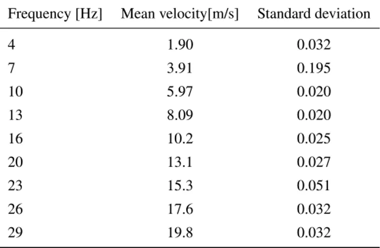
The analysis of the quality of the flow inside the wind tunnel shows the following results. The figure shows how the flow velocity changes in time for a given velocity. The values were obtained approximating the signal in time with a linear curve (using least square approach), and then the information was extrapolated from the slope of the linear curve. No great peaks are visible and are all in the order of 10−7_{so the flow can be considered stable in time. The following} table shows the standard deviation evaluated for every velocity measured

Frequency [Hz] Mean velocity[m/s] Standard deviation

4 1.90 0.032 7 3.91 0.195 10 5.97 0.020 13 8.09 0.020 16 10.2 0.025 20 13.1 0.027 23 15.3 0.051 26 17.6 0.032 29 19.8 0.032

Table 3.1: Value of standard deviation for each velocity. For all the velocities the value of the standard deviation is

Being the standard deviation an indicator of how much the data are spread from the mean (as expressed in the previous chapter), it can be seen as a parameter linked to the turbulence level inside the wind tunnel.

These results were obtained using the Pitot probe, that was fixed in a certain position inside the wind tunnel (bottom half of the cross section of the test section). The quality of the flow was also studied in space and not only in time. This step was made through the use of the hot wire. The acquisition were made in the centreline and top half of the test section. The results show a little difference in the velocity, thus the flow can be considered homogeneous also in space. This study was necessary in order to understand the quality of the flow and if the wind tunnel had critical velocities in which the flow can be unstable or separate. Be aware of the characteristic of the flow means better comprehend the results obtained in the future experiments.

Frequency [Hz] Velocity [m/s] Up Center 4 1.64 1.60 10 5.20 5.26 16 9.94 9.70 29 19.1 19.3

Table 3.2: Evaluation of the velocity inside the test section of the wind tunnel in two different points. The values are

almost the same, it can be said that the flow can be considered homogeneous in space

3.2

The Pitot probe

One of the most important tool in this type of experiment is the Pitot probe. The Pitot probe is necessary to measure the velocity of the flow inside the wind-tunnel. It measures the speed starting form the pressure measurement, thanks to two hole placed one in the stagnation point (total pressure) and one on the surface of the probe (static pressure). The relation between pressure and velocity is given by the Bernoulli equation: the total pressure is equal to the dynamic pressure and static one. Once it is known the total pressure and the static pressure it can be obtain the speed that is inside the dynamic pressure:

𝑃_𝑡= 𝑃_𝑠+ 𝑃_𝑑 (3.1) 𝑃_𝑡= 𝑃_𝑠+ 𝜌𝑉 2 2 (3.2) 𝑉 = √ 2(𝑃_𝑡− 𝑃_𝑠) 𝜌 (3.3)

The Pitot probes are useful to measure the main mode of the flow because it has a low dynamic response, for this reason it is mainly adopted to measure the main velocity. During the installation inside the wind tunnel, it must be pay close attention to the axial direction of the probe with respect to the flow. The Pitot probe in fact has a great directional sensitivity and some degrees of misalignment can produce wrong results.

Regarding the total pressure hole it must be paid attention on the shape of the velocity profile, in fact if the flow it is not homogeneous in the direction orthogonal to the probe axis some corrections must be applied. This because it was found that the flow particles measured are not the one who lays in that given coordinate but they are shifted down a

little. The opposite phenomenon happens in the case of wall interference. In the case of a velocity gradient there exist three different corrections obtained empirically.

Δ𝑦 𝑑 = 𝜀 𝜀= 0.15 (3.4) Δ𝑦 𝑑 = 0.18𝛼 ( 1 − 0.17𝛼2) 𝛼= 𝑑 2𝑈(𝑦_𝑐) 𝑑𝑈 𝑑𝑦 (3.5) Δ𝑦 𝑑 = 0.15 tanh 4 √ 𝛼 (3.6)

These are based on analytical displacement correction for a sphere in a velocity gradient.[15] In the case of wall inter-ference, instead:

𝛿_𝑤= 𝜖𝑑_𝑝 (3.7)

With 𝑑𝑝that is the diameter of the probe. Depending on the distance of the probe to the wall 𝜖 has different values:

⎧ ⎪ ⎪ ⎨ ⎪ ⎪ ⎩ 𝜖= 0.150 𝑑+<8 0.120 8 < 𝑑+_<110 0.085 110 < 𝑑+_<1600 (3.8)

In this study none of these corrections were necessary because the measurements were done in far from the wall and in absence of any velocity gradient. Also the static port can have some bad readings, these errors can be due to: orifice shape, orifice orientation, depth of the cavity and the surface orientation.

In order to look at all the quantities that can affect a bad reading on the static port a PI group is created:

Π = Δ𝑝 𝜏_𝑤 = 𝑓 (𝑑𝑠𝑢𝜏 𝜈 , 𝑑_𝑠 𝐷, 𝑀 , 𝑙_𝑠 𝑑_𝑠, 𝑑_𝑐 𝑑_𝑠, 𝜀 𝑑_𝑠 ) (3.9) to reduce the errors it is important to work with these quantities, or at least with the most of them.

Figure 3.3: B.J.McKeon, J.Li [15]Two type of Pitot total port interference: velocity gradient and wall interference. In

the first case the flow particle shift down, so the velocity read is higher than the real one, the opposite happens in the second case.

Figure 3.4: G.Bellani, A.Talamelli, Lecture notes [16]. Sketch of the static port in a Pitot probe. There exist lot of

variable that can interfere with the reading of the signal. It is very important to understand how the error can be reduced.

3.3

The hot-wire

The hot-wire is another tool useful to study the velocity of the flow in consideration. Unlike the Pitot probe, the hot wire has a much larger dynamic response, for this reason it is used in order to study fluctuation of the flow in the turbulent regime. The hot-wire consists in a tiny resistance connected to an arm of a Wheatstone bridge. Prior any experiments the calibration of the hot wire is necessary. Despite the Pitot probe that does not require any calibration because the reading of the pressure measurements gives immediately the values of the velocity, the hot wire needs to be calibrate in order to link any values of the output voltage to the velocity. The process of calibration starts with the evaluation of the resistance of the anemometer. The resistance of the anemometer is evaluated by subtracting the value of the resistance of the cable and Wheaston brdige, obtained by introducing a shortening probe, to the overall system: hot-wire, cable and Wheastone bridge. This first step is essential considering that due to the aging effect the value of the resistance can change, obtaining wrong measurements. Once the resistance has been evaluated different measure at different velocities are made. A key factor is to place close to each other the Pitot probe and the hot wire in order to know exactly the value of the velocity. After several measurements at different velocity, through an interpolation by point it is obtained the calibration curve that links the voltage and the velocity. The main drawback of the Pitot probe is its behaviour at low velocities, it has an offset that tents to disappear as the velocity increases. This is shown in the calibration curve, in fact it starts from a velocity equal to 0.6 m/s. This aspect is felt in the results in the regions where the velocity is low.

The physics behind the functioning of this device is related to the Joule effect: a current flows through a resistance that heats up, when this resistance is exposed to a flow there will be a heat loss due to convection, radiation and con-duction; know the amount of heat lost means know the velocity of the flow. As already said the three main component that cause the heat loss are: convection, it plays the main role, conduction and radiation are very small with respect the other one and sometimes they can be considered negligible. The governing equation is:

𝑑𝐸

Figure 3.5: Hot wire calibration curve obtained interpolating a 4th polynomial curve.

dE/dt=W-H Where 𝐸 = 𝐶𝑤𝑇𝑠and 𝑊 = 𝐼2𝑅𝑤. E is the thermal energy stored in the wire and it is defined as the

product between the heat capacity of the wire and the temperature; W is the power generating by the Joule effect and it is defined as the square of the current times the resistance of the wire, that is a function of the temperature of the wire itself[14]. The overall system is in equilibrium when 𝑊 = 𝐻. In particular, defining 𝑇𝑎as the ambient temperature

and knowing that 𝐼 = 𝑉 𝑅_𝑤: 𝑊 = 𝐻 (3.11) 𝑉2 𝑅_𝑤 = ℎ𝐴𝑤 ( 𝑇_𝑤− 𝑇_𝑎) (3.12)

the previous expression can be written by introducing a dimensionless number: the Nusselt number 𝑁𝑢 = ℎ𝑑 𝑘. 𝑉2 𝑅_𝑤 = 𝑘𝑁𝑢 𝐴_𝑤 𝑑 ( 𝑇_𝑤− 𝑇_𝑎) (3.13)

where k is the thermal conductivity of the fluid and d the characteristic length of the body, in this case the diameter of the wire. The Nusselt number is a function of several quantities:

𝑁 𝑢= 𝑁𝑢(𝑅𝑒, 𝑃 𝑟, 𝑀 .𝜏,…) (3.14) Where 𝑅𝑒= 𝑈 𝑑𝜌 𝜇 ; 𝑃 𝑟= 𝑐_𝑝𝜇 𝑘 ; 𝑀 = 𝑈 𝑎; 𝜏= 𝑇_𝑤− 𝑇_𝑟 𝑇₀ (3.15)

𝜏is called overheat ratio, with 𝑇_𝑟that is the recovery temperature and 𝑇0the stagnation temperature. The relation that

links all these variables is known as the King’s law and it is written as:

𝑁 𝑢= 𝐴′(𝜏)+ 𝐵′(𝜏)𝑅𝑒𝑛 (3.16)

Combining this expression with the one obtained in the previous equation it is obtained the equation for the calibration of the sensor:

(a) (b)

Figure 3.6: G.Bellani, A.Talamelli, Lecture notes [16].Relation between Nu and Re. At very low Reynolds number the

relation is dependent on the Grashof number.

The exponent n is in the range of 0.4/0.55. It is interesting to look at the relation between the Nusselt number and the Reynolds number. 𝐺𝑟= 𝑔𝛽𝐷 3(_𝑇 𝑠− 𝑇inf ) 𝜈2 (3.18)

The Grashof number is a dimensionless number and it is the ratio between buoyancy and viscous force acting on a fluid. g is the gravity acceleration, 𝛽 is the coefficient of thermal expansion of the wire, D the diameter of the wire, 𝑇𝑠the

temperature of the wire and 𝑇infthe temperature of the environment and 𝜈 is the kinematic viscosity of the fluid. If very low Reynolds number are reached it is possible to face some buoyancy effect, in order to avoid it the Reynolds number must be at least one third greater than the Grashof number. In standard case this means have a velocity greater than 0.07m/s.[16]

As well as the Pitot probe, also the hot wire anemometer is directional sensitive. It must be paid attention on the direction of the sensor with respect the flow. There are two coefficients that takes into account the yaw (𝜃) and pitch (𝛼) components of the velocity:

𝑈_{𝑒𝑓 𝑓}2 = 𝑈_𝑥2+ 𝑘2𝑈_𝑦2+ ℎ2𝑈_𝑧2 (3.19)

This velocity is called “effective cooling velocity”, that is different from the velocity acquired in the computer, in fact the velocity acquired is the perpendicular component of the velocity. The previous expression was found taking the components of the velocity in the normal and tangential plane with respect to the wire. In the case of x-y plane, the angular response is characterized by a strong decrease of effective velocity when the angle 𝛼 increases. This can be explained thanks to the heat transfer of a cylinder, the heat transfer is highest when the flow is normal to the cylinder. This is called Champagne law:

Figure 3.7: G.Bellani, A.Talamelli, Lecture notes [16]. Directional sensitivity of the hot wire anemometer. The yaw

and pitch angle are the ones that can affect the reading of the signal.

In the x-z plane the angular response is expressed by Gilmore:

𝑈_{𝑒𝑓 𝑓}2 = 𝑈2(cos 𝜃2+ ℎ2sin 𝜃2)= 𝑈_𝑥2+ ℎ2𝑈_𝑧2 (3.21)

Usually the value of k is around 0.1, regarding h it is in the range between 1 and 1.1. This is due to the effect of the wire prongs that, in case of binomial direction of the flow, cause an acceleration of the flow in the location of the wire. The family of the hot-wire can be divided in three groups depending on the principle of functioning: Constant Current Anemometer (CCA), Constant Voltage Anemometer (CVA) and Constant Temperature Anemometer (CTA). As the name suggests, the CCA keeps the current constant through the sensor. This type of Hot-wire is not so spread, it has several drawbacks such as: highly risk of probe burnout, low frequency response and the output of the sensor decrease with the increasing of the velocity. The main advantage of this configuration is the low level of noise. The CVA keeps constant the voltage through the sensor, it has a large response and high frequency response. The CTA keeps the temperature constant, it is the configuration adopted for this experiment. It has a great dynamic response but it is very susceptible to the noise. The frequency response of the CTA is determined by the square wave test. The hot wire receives a train of square waves, depending on the settling time (time in which the signal returns in the previous configuration) the frequency response is determined. Regarding the CCA the frequency response can be obtained by:

𝑀 = 𝑐𝑤𝜌𝑤𝛼𝑅𝑑 2

𝑘_𝑓𝑁 𝑢 (3.22)

Where 𝑐𝑤is the heat capacity of the wire, 𝜌𝑤is the density of the wire material, 𝛼𝑅is the thermal coefficient of the wire,