Effects of settlements on Pombalino buildings (Lisbon) taking into account soil-structure interaction

ALMA MATER STUDIORUM - UNIVERSITÀ DI BOLOGNA

SCUOLA DI INGEGNERIA E ARCHITETTURA

DIPARTIMENTO DI INGEGNERIA CIVILE, CHIMICA, AMBIENTALE E DEI

MATERIALI

CORSO DI LAUREA MAGISTRALE IN INGEGNERIA PER L’AMBIENTE E IL

TERRITORIO

TESI DI LAUREA

in

Opere in Sotterraneo M

Effects of settlements on Pombalino buildings (Lisbon) taking into

account soil-structure interaction

CANDIDATO:

RELATORE:

Giacomo Rigon

Prof.ssa Ing. Daniela Boldini

CORRELATORE:

Prof. Ing. Rui Carrilho Gomes

Anno Accademico 2017/2018

Sessione III

Abstract

Failures and damages to infrastructures and buildings may occur near an excavation. One of the causes is the lowering of the water level, which is necessary to perform the excavation or to maintain service. Nowadays the development of underground infrastructures requires a careful analysis of the soil- struc-ture interaction in order to preserve the strucstruc-tures’ integrity. This analysis acquires a peculiar relevance when the excavation is done in densely occupied areas or near old buildings. This thesis, developed at Instituto Superior T´ecnico (IST), presents the case of the Pombalino building in the downtown of Lis-bon which, in the last years, has seen an increase in the construction of underground structures. The Pombalino, constructed in the second half of the XVII century, is the symbol of the city’s reconstruction after the 1755’s earthquake. It is characterized by the Pombalino cage, a wooden structure installed to resist the seismic action; however nowadays this structure has become an element of weakness in the masonry. The work of the thesis aims to analyze the interaction between the soil and the Pombalino building when in the nearby area a drawdown of water level is carried out . The analysis is conducted with the finite element code PLAXIS 2D and focuses on the assessment of the movements under the Pombalino building and on the deformations induced on the facade of the building. The Pombalino cage is simulated thanks to the Jointed Masonry constituitve model, which allows to simulate the weaknesses’ directions defined by the wooden beams and enables to quantify the deformations entity.

Keywords

Water drawdown, displacements, excavation, finite element, PLAXIS;

Resumo

Na vizinhanc¸a de uma escavac¸˜ao pode ocorrer deformac¸˜oes excessivas em infraestruturas e construc¸˜oes. Uma das causas ´e o rebaixamento do n´ıvel fre´atico necess´ario para realizar a escavac¸˜ao ou durante a fase de servic¸o. Hoje em dia, a criac¸˜ao de estruturas subterrˆaneas exige uma cuidadosa an´alise sobre a interac¸˜ao terreno-estrutura, a fim de salvaguardar a integridade da estrutura. Esta an´alise torna-se fundamental quando a escavac¸˜ao ´e feita em ´areas densamente ocupadas ou na presenc¸a de edif´ıcios antigos. Esta tese analisa o caso do um edif´ıcio pombalino do centro hist´orico de Lisboa onde, nos ´ultimos anos, se tem desenvolvido a construc¸˜ao de estruturas subterrˆaneas. O edif´ıcio Pombalino, que remonta `a segunda metade do s´eculo XVIII, representa o s´ımbolo da reconstruc¸˜ao da cidade ap´os o sismo do ano 1755, e caracteriza-se pela presenc¸a da gaiola pombalina, uma estrutura de madeira criada naquela altura para resistir `a actividade sismica, que hoje torna-se elemento de fraqueza da alvenaria devido `a sua degradac¸˜ao. Esta trabalho analisa a interac¸˜ao entre o terreno e o edif´ıcio pom-balino quando nas proximidades ´e efectuada o rebaixamento do n´ıvel fre´atico. A an´alise ´e efetuada atrav´es do programa PLAXIS 2D e concentra-se na determinac¸˜ao dos assentamentos do edif´ıcio pom-balino e nas deformac¸˜oes induzidas na fachada do pr´edio. A gaiola pombalina ´e simulada atrav´es do modelo num´erico Joint Masonry que permite simular as direc¸˜oes de fraqueza determinadas pelas vigas de madeira, e permite avaliar os danos no edif´ıcio.

Palavras Chave

Rebaixamento do n´ıvel fre´atico, deslocamentos, escavac¸˜ao, elemento finito, PLAXIS;

Abstract

In prossimit`a di uno scavo possono verificarsi cedimenti e danni ad infrastrutture ed edifici. Una delle cause `e l’abbassamento del livello di falda necessario per eseguire lo scavo. Oggi giorno lo sviluppo di infrastrutture sotterranee richiede un’attenta analisi dell’interazione terreno-struttura al fine di preser-vare l’integrit`a delle strutture. Tale analisi assume particolare importanza quando lo scavo `e eseguito in aree congestionate o quando si `e in presenza di antichi edifici. Questa tesi, sviluppata presso l’Instituto Superior T`ecnico, presenta il caso dell’edificio Pombalino nel centro storico di Lisbona in cui negli ul-timi anni `e cresciuta la costruzione di infrastrutture sotterranee. Il Pombalino, risalente alla seconda met`a del ’700 rappresenta il simbolo della ricostruzione della citt`a dopo il sisma del 1755 e si contrad-distingue per la presenza della gabbia pombalina, una struttura lignea all’epoca installata per resistere all’azione sismica, ma oggi divenuta un elemento di debolezza della muratura. Il lavoro di tesi intende analizzare l’interazione tra il terreno e l’edificio Pombalino quando nelle vicinanze viene eseguita una riduzione del livello di falda. L’analisi `e condotta con il codice agli elementi finiti PLAXIS 2D e si concentra sulla valutazione degli spostamenti al di sotto del Pombalino e sulle deformazioni indotte nella facciata dell’edificio. La gabbia pombalina `e simulata attraverso il modello numerico Joint Masonry Model il quale permette di simulare le direzioni di debolezza definite dalle travi in legno e consente di stimare l’entit`a delle deformazioni.

Keywords

Abbassamento falda, cedimenti, scavo, elementi finiti, PLAXIS 2D;

Contents

2.2 Pombalino building . . . 12

2.3 Lisbon downtown settlements . . . 14

3 Numerical simulation 21 3.1 Finite element method (FEM) . . . 23

3.2 Constitutive models . . . 23

3.2.1 Hardening Soil model and Hardening Soil model with small-strain stiffness (HSsmall) 24 3.2.1.A HSsmall simulation . . . 28

3.2.2 Jointed Rock Model and Masonry Model. . . 31

3.2.2.A Masonry model simulation . . . 37

3.3 Drainage conditions simulated in PLAXIS 2D . . . 41

3.3.1 Drained and undrained analysis . . . 42

3.4 2D Model . . . 43

3.4.1 Ground model . . . 43

3.4.1.A Geometry. . . 43

3.4.1.B Properties . . . 44

3.4.1.C Results . . . 45

3.4.2 2D with underground structure . . . 47

3.4.2.A Geometry. . . 47

3.4.2.B Properties . . . 47

3.4.2.C Results . . . 48 vii

4 Case study 55

4.1 Modeling Pombalino facade . . . 57

4.1.1 Geometry of Pombalino facade . . . 57

4.1.2 Properties of Pombalino facade. . . 58

4.1.3 Soil profile. . . 59

4.1.4 Soil properties . . . 61

4.2 Drawdown of water level . . . 61

4.3 Results . . . 63

List of Figures

2.1 Left: surface geology of the Baixa area. Right: digital terrain model (DTM) obtained from a 1:1000 survey scale. Dashed black lines separate the three defined zones (north, central

and south) [1]. . . 8

2.2 Left: thickness of anthropogenic deposits (left) and alluvial deposits (right) in Baixa [1]. . . 9

2.3 Distribution of NSPT values in the alluvial deposits for the three zones for different depths (left) and with depth clayey and sandy materials (right) [1]. . . 11

2.4 Example of a Pombalino building [3]. . . 12

2.5 Foundations and frontals in a Pombalino building [4]. . . 13

2.6 Example of wood piles in Pombalino building (left) longitudinal section and cross section (right). . . 13

2.7 Example of frontals in a Pombalino building (ovoodocorvo.blogspot.com). . . 14

2.8 Location of piezometers (blu), marks (pink) and leveling slabs (green) installed in Lisbon downtown from March 2004 to December 2010 [8]. . . 15

2.9 Variation of water table in the alluvium layer from March 2004 to December 2010 [7]. . . . 16

2.10 Variation of water table in the miocene layer from March 2004 to December 2010 [7]. . . . 17

2.11 Map of underground constructions in Lisbon downtown [7]. . . 18

2.12 Contour of vertical displacements measured from 2004 to 2010 in Lisbon downtown [8]. . 19

2.13 Behavior of surface marks, leveling slabs and measuring points recorded in Lisbon down-town [8]. . . 20

3.1 Hyperbolic stress-strain relation in primary loading for a standard drained triaxial test [12]. 25 3.2 Results from theHardin-Drnevich relationship compared to test data by Santos & Correia (2001) [12]. . . 27

3.3 Rigidity modulus E0, Eurand E50in a triaxial test for HSsmall model [12]. . . 27

3.4 Triaxial test for alluvium layer: q versus "1and "v versus "1. . . 29

3.5 Triaxial test for alluvium layer: "vversus "1. . . 29

3.6 Triaxial test for alluvium layer: ⌧ versus 0_{. . . . 30}

3.7 Stiffness degradation curve. . . 30

3.8 Idea behind Joint Rock model [12]. . . 31

3.9 Global and local coordinate systems in 2D conditions for the joints [10]. . . 32

3.10 Definition of ↵1and ↵2[12]. . . 32

3.11 Example of failure directions for JR model in PLAXIS 2D [12]. . . 33

3.12 Definition of Plane 1 and Plane 2 in the Modified Jointed Rock Model [10].. . . 34

3.13 Stress state on a portion of the masonry wall (left) and in the single brick (rigth) [10]. . . . 34

3.14 Geometry of panels tested. Dimensions are given in meters. . . 37

3.15 Total principal strain "1for set a. . . 39

3.16 Total principal strain "3for set a. . . 39

3.17 Total principal strain "1for set b. . . 39

3.18 Total principal strain "3for set b. . . 40

3.19 Total principal strain "1for set c. . . 40

3.20 Total principal strain "3for set c. . . 40

3.21 Geometry of the model without underground structure. . . 44

3.22 Principal vertical effective stress (blu) and principal horizontal effective stress (orange) at the end of water drawdown. . . 46

3.23 Shadings (right) and contour lines (left) of total displacement at the end of calculation. . . 46

3.24 Geometry of the model with underground structure.. . . 47

3.25 Evolution of water drawdown surrounding the parking area. . . 49

3.26 Evolution of total displacements surrounding the parking area. . . 49

3.27 Evolution of vertical displacements surrounding the parking area. . . 50

3.28 Evolution of horizontal displacements surrounding the parking area. . . 50

3.29 Deformed mesh at the end of calculation. . . 51

3.30 Contour lines of total displacements at the end of water drawdown. . . 51

3.31 Arrows of total displacements at the end of water drawdown. . . 52

3.32 Water pressure at the end of calculation.. . . 52

4.6 Arrows of total displacements after the Pombalino and parking area activation (left) and

at the end of water level drawdown (right). . . 63

4.7 Evolution of total displacements in the entire domain.. . . 64

4.8 Evolution of total displacements induced only by water drawdown under Pombalino build-ing. . . 65

4.9 Evolution of total displacements under Pombalino building. . . 66

4.10 Evolution of water drawdown under Pombalino building. . . 67

4.11 Evolution of total displacements under Pombalino building. . . 67

4.12 Evolution of vertical displacements under Pombalino building. . . 68

4.13 Evolution of horizontal displacements under Pombalino building. . . 68

4.14 Evolution of total strain "1(left) and "3(right) of Pombalino building ground floor at the end of water drawdown.. . . 69

4.15 Evolution of total strain "1(left) and "3(right) of Pombalino building upper floors at the end of water drawdown.. . . 69

4.16 Evolution of total strain "1(left) and "3(right) of Pombalino building openings at the end of water drawdown.. . . 70

4.17 The generated deformed mesh for the case study. . . 70

4.18 Geometry considered to calculate distortion . . . 71

4.19 Intensity of damage as a function of distortion and soil extension deformation "h (modi-fied by Boscarding & Cording 1989) [13] . . . 72

4.20 From left to right: total strain "1, total strain "3and deformed mesh of Pombalino building in relation to total displacements at the end of water drawdowns. . . 72

List of Tables

3.1 Parameters for the Hardening Soil model. . . 26

3.2 Parameters of the Hardening Soil with small-strain stiffness model used in the triaxial test. 28 3.3 Parameters of the Jointed Rock model. . . 33

3.4 Parameters of the Masonry Jointed Model. . . 36

3.5 Parameters of the Masonry Jointed Model for the tests. . . 38

3.6 Soil layers in Restauradores square. . . 43

3.7 Parameters of ZG1 with Mohr Coulomb model. . . 44

3.8 Parameters of ZG2 and ZG3 with Hardening Soil with small-strain stiffness model. . . 45

3.9 Material properties of the diaphragm wall. . . 48

4.1 Parameters of Pombalino building foundations and ground floor.. . . 59

4.2 Parameters of Pombalino building upper floors. . . 59

4.3 Parameters of ZG2 and ZG3 with Hardening Soil with small-strain stiffness model. . . 62

4.4 Damage categories associated with the achievement of extension limit deformation in the structure (modified by Boscarding & Cording 1989) [13]. . . 72

Acronyms and symbols

FEM Finite Element Methood

IST Instituto Superior T´ecnico

JRM Jointed Rock Model

MM Masonry Model

MC Mohr-Coulomb criterium

HS Hardening Soil Model

HSsmall Hardening Soil with small-strain stiffness model

SPT Standard Penetration Test ACross section

cCohesion dThickness eVoid ratio

EYoung’s modulus EoedOedometer modulus

pIsotropic stress or mean stress P OP Pre overburden pressure qDeviatoric stress uTotal displacements uxHorizontal displacements uyVertical displacements Unit weight Shear strain Increment

✏Vector with cartesian strain components ✏q Deviatoric strain ✏vVolumetric strain ⌫Poisson’s ratio 'Friction angle ⇠Dilatancy angle xv

1

Introduction

Contents

In this chapter a general description of the subject involved in the thesis, its aim and its organization are summed up.

1.1 General overview

When an excavation is carried out, damages may be induced to buildings and infrastructures in the surrounding area. This effect gains more relevance when the soil excavated is close to cities centers or congested areas. Surface movements of the soil can generate cracks on building facade, especially in case of old buildings with historical and artistic value.

After the earthquake of 1755, downtown of Lisbon was reconstructed with the application of the first modern seismic resistant system. Structural elements strongly resistant to horizontal motions were used to build the well known Pombalino building. It is has a regular and simple shape which gained historical and cultural value year after year. It has become the symbol of the reconstruction of Lisbon.

Investigations show that over the years ground settlements and fractures in Pombalino buildings have occurred. It is likely that the construction of underground infrastructures such as metro stations and parking areas might have contributed. In these situations the overburden removal generates stress relief. Moreover these types of work may require the pumping of ground water and consequently the variation of the soil stress state can produce subsidence in the ground.

This work studies a building in Lisbon downtown, with attention focused on a generic Pombalino building located in the proximity of Restauradores Square. The soil structure interaction is studied with a 2D finite element software and results are compared with total displacements measured from 2004 to 2010 by the Municipality of Lisbon.

1.2 Goal

The main goal of this dissertation is to investigate displacements under a Pombalino building when in the proximity an excavation is carried out and the water table is subjected to a sequence of drawdowns. The behaviour of the building is simulated through a numerical model which allows to characterize the response of masonry expose to the displacement field induced by the water level decrease. In other words the objective is to investigate the impact of water table drawdown and facade’s damages.

1.3 Thesis organization

This document is divided in five chapters. In the first one is presented a general overview. In chapter two the geotechnical and geological characterization of Lisbon downtown is presented. Further the

main features of Pombalino building and a case history are presented. Chapter three is about the finite element theory and the numerical models used in the simulation. In order to characterize the response of the model some tests have been carried out and their results are presented. Next in chapter four the simulation of the case study is illustrated in detail. Results are shown and commented. In the end final conclusions and future developments are reported.

2

Lisbon downtown

Contents

2.1 Geological and geotechnical characterization of Lisbon downtown . . . . 7

2.2 Pombalino building . . . 12

2.3 Lisbon downtown settlements. . . 14

This chapter contains the results of the geological and geotechnical characterization related to the area of this work. After the description of the main features of Pombalino building a brief summary of measurements carried in Lisbon downtown is presented.

2.1 Geological and geotechnical characterization of Lisbon

down-town

During its history, Lisbon has been affected by several medium to strong earthquakes that caused con-siderable damage and produced large economic and social impacts. In particular, the very large and well known November 1st, 1755, earthquake (M 8)caused the complete destruction of its downtown area (Baixa), which was reconstructed with the application of the first implemented seismic resistant system [1]. Eurocode 8 presents the classification of soil into a small number of classes according to the value of the average shear-wave velocity in the upper 30 m of the surface (vs,30). A geotechnical

characterization of Lisbon downtown was performed based on the analysis of Standard Penetration Test (SPT) data compiled in the geological and geotechnical database. This database, allows the definition of 2D geological profiles used for estimating the thickness of the shallower layers. The shear-wave velocities for each layer were estimated from empirical correlations using mean SPT values computed from the statistical evaluation of the compiled data. Baixa, the downtown of Lisbon, has been occupied since prehistorical times because its strategic geographical location. After the earthquake of 1755 the most damaged area was Baixa, not only due to the site response to the strong ground motion but also due to the tsunami that followed and the fire triggered by the earthquake. Marquˆes de Pombal led the planning and reconstruction of Lisbon downtown, with the help of engineers and architects Manuel da Maria, Eug´enio dos Santos and Carlos Mardel [2]. The new town was built over the ruins and, as a consequence of the great volume of debris, a thick layer of man-made (anthropogenic) materials, locally buried in the soft alluvial deposits, covered the creek area. Due to this process, the local coastline was artificially moved closer to its present-day location [1].

The Baixa area, located in the northern estuarine margin of the Tagus River, corresponds to the fluvial outlet of a 6, 2 km2 _{elongated basin cut in the Miocene bedrock. The valley is filled by a thick layer of}

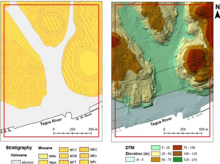
alluvial sediments (normally consolidated silty sands and organic silty clays) and it is surrounded by three gentle hills [1]. The main lithologies of Baixa are showed in figure2.1. They consist of:

• silty clayey soils and calcarenites (MPr and MFT);

• fine micaceous sandy and silty sandy soils (MEs, MQB and Mpm); • limestones, calcarenites and coquinites (MEC, MCV and MMu);

Figure 2.1: Left: surface geology of the Baixa area. Right: digital terrain model (DTM) obtained from a 1:1000 survey scale. Dashed black lines separate the three defined zones (north, central and south) [1].

As part of the GeoSIS Lx research project, a geological and geotechnical database has been devel-oped to include in situ investigation data (borehole interpretation, sampling and geotechnical measure-ments) and laboratory test results [1]. Based on the interpretation of the geological map and the retrieval of database information, the geological model was set. The registered data points were interpolated for the whole downtown Lisbon area, through a kriging algorithm, to determine the surfaces representing the lower boundary of each formation of interest [1]. Figure2.2shows anthropogenic deposits (left) and alluvial deposits (right) in Baixa.

Figure 2.2: Left: thickness of anthropogenic deposits (left) and alluvial deposits (right) in Baixa [1].

Results of Standard Penetration Test (SPT) tests and lithology has been studied to perform the geotechnical characterization. The irregular spatial distribution was one of the main difficulties of the analysis. A total of 376 boreholes were selected for analysis in the Baixa area, which included 1398 NSP T data values. In order to check the spatial variations of geotechnical properties due to the

geolog-ical genesis and evolution of alluvial sedimentation, the area investigated was divided in three different zones (northern, central and southern) as showed in figure2.1.

The alluvial deposits are characterized by the presence of lenticular bodies and significant lateral and vertical facies variations. The main lithological facies include soft to stiff silt and clay, loose to dense sands, and a range of transitional lithologies. The NSP T values indicate the presence of normally and

slightly overconsolidated soils [1]. NSP T presents a remarkable irregularity. According to the authors it

can be interpreted as a result of the vertical and lateral lithological variation within the lenticular bodies. Figure2.3shows the distribution of NSP T with depth (right) and values of NSP T at different depth (left)

for the alluvium deposits in the three zones analyzed.

The anthropogenic deposits, which consist even on debris from the 1755 earthquake, present a heterogeneous composition. The relative distribution of NSP T slightly increases with depth, due to the

increasing overburden pressure.

The Miocene bedrock is characterized by a sequence of sands, clays, marls, calcarenites, coquinites and limestones, with important vertical and lateral facies variations. The NSP T values indicate the

presence of overconsolidated stiff soils and soft rocks. The large range of values is a consequence of the heterogeneity in lithology and of the superficial degradation of the mechanical properties of the overconsolidated Miocene materials [1].

Figure 2.3: Distribution of NSPT values in the alluvial deposits for the three zones for different depths (left) and with depth clayey and sandy materials (right) [1].

2.2 Pombalino building

After the 1775 earthquake engineers and architects Manuel da Maria, Eug´enio dos Santos and Carlos Mardel started to plan the construction of the new downtown of Lisbon. They decided to demolish the ruins and then to use structural elements with a relevant resistance to horizontal actions. The results were buildings with a regular and simple shape commonly called Pombalino (Figure2.4).

Figure 2.4: Example of a Pombalino building [3].

The downtown of Lisbon is composed of approximately sixty blocks consisting in average of seven buildings. Within each block, the buildings are constructed side by side, sharing the same gable walls. [3]. Pombalino is usually founded in short wood piles connected by arches where they settled the masonry (figure2.6).

Figure 2.5: Foundations and frontals in a Pombalino building [4].

Figure 2.6: Example of wood piles in Pombalino building (left) longitudinal section and cross section (right).

Figure 2.7: Example of frontals in a Pombalino building (ovoodocorvo.blogspot.com).

joined by lime. The facade presents a large number of windows. Figure2.5resumes the main features of Pombalino building.

2.3 Lisbon downtown settlements

With the aim of evaluate the state of Baixa conservation, in 2003 the Municipality of Lisbon started to monitor the groundwater levels of downtown to asses their relation with ground settlements. To do that sixteen open standpipe piezometers and surface topographic marks were installed. Also leveling slabs were used to monitor vertical movements of the buildings (figure2.8). Figures2.9and2.10show water table variations from March 2004 to December 2010 respectively in the alluvium layer and the miocene layer. The local lowering of the water table, due to the pumping for the construction of underground infrastructures, is one of the main causes of the settlements [8]. When porewater pressure decreases, the effective stress increases causing settlements.

Figure 2.8: Location of piezometers (blu), marks (pink) and leveling slabs (green) installed in Lisbon downtown from March 2004 to December 2010 [8].

Figure 2.10: Variation of water table in the miocene layer from March 2004 to December 2010 [7].

Figure 2.12: Contour of vertical displacements measured from 2004 to 2010 in Lisbon downtown [8].

The vertical displacements measured from 2004 to 2010 were used to generate the contour map shown in figure2.12. Three areas with the same magnitude of displacements are visible, corresponding to Restauradores Square (M53 north west), Figueira Square (M41 southern than previous area) and Martim Moniz Square (M50 north east). These marks are situated close to the parking area and subway metro station, as can be seen in figure2.11.

Figure 2.13: Behavior of surface marks, leveling slabs and measuring points recorded in Lisbon downtown [8].

According to Cruz [8], it is possible to distinguish three types of settlements trends of Lisbon down-town area in the period from 1956 to 2008 (figure2.13). Group A represents part of the surface marks that exhibit a stabilized behavior, with no visible tendencies to increase settling. Group B correspond to a serie of points that show a slight tendency to increase settlements. The mark number M53 correspond-ing to Restauradores Squared belongs to Group B and shows a tendency to amplify displacements up to a value of 0, 05 m in 2028 [8]. Finally Group C has an higher rate of settlements than Group B. It differs from Group B for the rate of displacements.

3

Numerical simulation

Contents

3.1 Finite element method (FEM) . . . 23

3.2 Constitutive models. . . 23

3.3 Drainage conditions simulated in PLAXIS 2D . . . 41

3.4 2D Model . . . 43

In this chapter the finite element method (FEM) is presented. It follows a description of the main constitutive models that this work takes into account. In conclusion a 2D case with PLAXIS of a water drawdown in a soil deposit is proposed.

3.1 Finite element method (FEM)

The Finite Element Methood (FEM) is a numerical method for obtaining approximate solutions to a wide variety of engineering problems. Its formulation consists on a system of algebraic equations. The method yields approximate values of the unknowns at discrete number of points over the domain. The geometry of the problem is divided in smaller parts called finite elements. The system of algebraic equations is composed by the simple equations that model each finite elements. To approximate a solution FEM minimizes an error function associated to the calculation of the unknowns.

The software that I used in this thesis for the study of the soil and building interaction is PLAXIS 2D. The geometry of the boundary value problem under investigation should be defined and quanti-fied. Simplifications and approximations may be necessary during this process. This geometry is then replaced by an equivalent finite element mesh which is composed of small regions called finite ele-ments [9]. Usually the finite elements corresponds to triangular or quadrilateral in shape for two di-mensional problems. Nodes are key points of the finite element because their coordinates define the geometry of the element. Each finite element is systematically numbered in order to refer to the complete finite element mesh. It is important to underline that the geometry of the boundary value problem should be approximated as accurately as possible. For that reason in the case of discontinuities, interfaces be-tween materials with different properties and applied boundary conditions is possible to introduce new finite elements and nodes. In order to obtain accurate solutions, these zones require a reined mesh of smaller elements [9]. The situation is more complex for general nonlinear material behaviour, since the final solution may depend, for example, on the previous loading history [9]. It is necessary to define with accuracy the boundary conditions and the material properties. For these materials the loading history should be divided into a number of solution increments and a separate finite element solution obtained for each increment. The incremental global stiffness matrix is not constant but varies during the incre-ment with stress and or strain. For that reason a solution strategy is necessary to take into account this changes in material behaviour.

3.2 Constitutive models

It is well known that soil and rock behaviour is highly non-linear and complex. This non-linear stress-strain behaviour can be modeled at several levels of sophistication. The constitutive models have a great

influence on the results obtained in the modeling. The more complex models tend to represent better the behavior of the materials, however the amount of parameters needed is higher and some don’t have physical meaning. Moreover data for their correct definition are not always available. PLAXIS supports different models to simulate the behaviour of soil. Due to the complexity of the strain-strain relationship and the small strain induced in the soil, in this work the following models have been used: Hardening Soil small-strain stiffness (HSsmall), and Masonry model, a modeled version of the Jointed Rock model [10]. In the next section these models are described in detail.

3.2.1 Hardening Soil model and Hardening Soil model with small-strain

stiff-ness (HSsmall)

To simulate the soil behaviour it is possible to use the Hardening Soil with small-strain stiffness model (HSsmall) which is an elastoplastic type of hyperbolic model, formulated in the framework of shear hardening plasticity. It involves compression hardening to represent irreversible compaction of soil under compression. Moreover it allows for a more realistic representation of soil behavior, particularly in the consideration of unload and reload cycles such as successive stages of excavation [11].

Unlike to an elastic perfectly-plastic model, the yield surface of a hardening plasticity model is not fixed in principal stress space, but it can expand due to plastic straining. Distinction can be made between two main types of hardening, namely shear hardening and compression hardening. The first one is used to model irreversible strains due to primary deviatoric loading. The second hardening is used to model irreversible plastic strains due to primary compression in oedometer loading and isotropic loading. The Hardening Soil Model (HS) considers both types of hardening.

Some basic characteristics of the model are:

• stress dependent stiffness according to a power law (parameter m); • plastic straining due to primary deviatoric loading (parameter Eref

50 );

• plastic straining due to primary compression (parameter Eref oed);

where Eiis related to E50by:

Ei=

2E50

2 Rf (3.2)

The parameter E50 is the confining stress dependent stiffness modulus for primary loading and is

provided by equation3.3:

E50= E50ref

✓ _{c cos ' 0}

3sin '

c cos ' + pref_{sin '}

◆m

(3.3) where Eref

50 is a reference stiffness modulus corresponding to the reference confining pref.

Figure 3.1: Hyperbolic stress-strain relation in primary loading for a standard drained triaxial test [12].

The parameters for the Hardening Soil model are listed in table3.1.

To simulate small-strain stiffness two additional parameters which describe the behaviour of stiffness in the range of small deformations are needed:

• the initial or very small-strain shear modulus G0;

• the shear strain level 0.7 at which the secant shear modulus Gsis reduced to about 70% of G0;

Test data highlights that the stress-strain curve for small strains can be described by a simple hyper-bolic law. The Hardin-Drnevich relationship (eq3.4) describes well this phenomenon:

Gs G0 = 1 1 +_| r| (3.4) where ris the threshold shear strain and is given by:

r=

⌧max

G0 (3.5)

Table 3.1: Parameters for the Hardening Soil model.

Symbol Meaning Unit

Failure parameters as in MC model

c (Effective) cohesion kN/m2

' (Effective) angle of internal friction Angle of internal friction

t Tension cut-off and tensile strength kN/m2

Basic parameters for soil stiffness

E₅₀ref Secant stiffness in standard drained triaxial test kN/m2

E_oedref Tangent stiffness for primary oedometer loading kN/m2

Eref

ur Unloading / reloading stiffness kN/m2

m Power for stress-level dependency of stiffness Advanced parameters

⌫ur Poisson’s ratio for unloading-reloading (default ⌫ur= 0, 2)

pref _{Reference stress stiffnesses (default p}ref _{= 100) kN/m}2

Knc

0 K0-value for normal consolidation (default K0nc= 1 sin ')

Rf Failure ratio qf/qa (default Rf= 0, 9)

tension Tensile strength (default tension= 0) kN/m2

where ⌧maxis the shear stress at failure.

Equations 3.4and3.5can be considered for large strains. More straightforward and less prone to error is the use of a smaller threshold shear strain. Santos & Correia (2001), for example suggest to use the shear strain r = 0.7 at which the secant shear modulus Gs is reduced to about 70% of its initial

value [12]. Equation3.4become:

Gs

G0

= 1

1 + a_{| r|} (3.6)

If a value of a equal to 0, 385 is considered, a value of Gs

G0 equal to 0, 772 is reached.

G0can be determined by measuring the tensions and deformations considering ”small” loads or by

measuring shear wave’s velocity (wave propagation theory). In PLAXIS ⌫ur is considered constant so

Figure 3.2: Results from theHardin-Drnevich relationship compared to test data by Santos & Correia (2001) [12]. Where: K( , IP ) = 0, 5  1 + tanh ✓ ln ✓_{0, 000102 + n(IP )}◆0,492◆ (3.9) m( , IP ) m0= 0, 272  1 tanh ✓ ln ✓_{0, 000556}◆0,4◆ exp ( 0, 0145IP1,3) (3.10) Figure3.3illustrates for HSsmall model the rigidity modulus E0, Eurand E50in a triaxial test.

Figure 3.3: Rigidity modulus E0, Eurand E50in a triaxial test for HSsmall model [12].

3.2.1.A HSsmall simulation

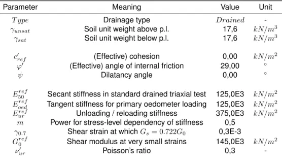
In order to characterize the response of the numerical model a triaxial test was carried out in PLAXIS for alluvium layer. Parameters used in the test were obtained by the geological surveys of GeoSIS Lx research project and they are presented in table3.2. They are representative of the alluvium layer ZG2 considered in the case study. PLAXIS 2D function SoilTest enables to simulate real life soil tests such as triaxial test which lets to test soil properties while controlling the stresses applied in the vertical and horizontal directions. The vertical preconsolidation stress 1and the initial effective stress 03are equal

to 100 kP a.

Table 3.2: Parameters of the Hardening Soil with small-strain stiffness model used in the triaxial test.

Parameter Meaning Value Unit

T ype Drainage type Drained

-unsat Soil unit weight above p.l. 17,6 kN/m3 sat Soil unit weight below p.l. 17,6 kN/m3

c0ref (Effective) cohesion 0,00 kN/m2

'0 (Effective) angle of internal friction 29,00 Dilatancy angle 0,00

Eref₅₀ Secant stiffness in standard drained triaxial test 125,0E3 kN/m2

Eref_oed Tangent stiffness for primary oedometer loading 125,0E3 kN/m2

Eref

ur Unloading / reloading stiffness 375,0E3 kN/m2

m Power for stress-level dependency of stiffness 0,5

0.7 Shear strain at which Gs= 0.722G0 0,3E-3

Gref0 Shear modulus at very small strains 145,0E3 kN/m2

⌫ur0 Poisson’s ratio 0,3

-Results of the triaxial compression isotropic test (drained conditions), are showed in figures3.4,3.5

and3.6. In the first one is possible to observe that the deviator stress progressively increases until large deformations of the order of 0, 7% are attained. For small values of "1 soil behaviour can be assume

elastic. Simultaneously the specimen continuously reduces its volume and only at large deformations shear strains occur without any further volume change (figure 3.5). Figure3.6 shows the failure line

Figure 3.4: Triaxial test for alluvium layer: q versus "1and "vversus "1.

Figure 3.5: Triaxial test for alluvium layer: "vversus "1.

3.2.2 Jointed Rock Model and Masonry Model

Anisotropy is the property of being directionally dependent, which involves different properties in dif-ferent directions. Materials characterized by anisotropy respond difdif-ferently when subjected to specific conditions in one direction rather than another [12]. The Jointed Rock model Jointed Rock Model (JRM) simulates plastic anisotropy by using different strength properties in different directions.

Figure 3.8: Idea behind Joint Rock model [12].

Joint Rock is an anisotropic elastic-perfectly plastic model where plastic shearing can only occur in a limited number of shearing directions. For that reason it is assumed that the rock is intact and an optional stratification direction is present [12]. The intact rock is considered as an anisotropic elastic material characterized by five parameters and a direction.

The Joint Rock Model considers in its formulation a maximum of three different rock-mass discontinu-ity planes along which a Mohr-Coulomb Mohr-Coulomb criterium (MC) yield criterion holds with tension cut-off. A maximum of three sliding directions can be chosen and they can have different shear strength properties. Figure3.9shows coordinate systems in 2D conditions for joints. The MC and tensile-cut off yield functions are defined respectively by equations3.11and3.12for i = 1...np0:

fic =|⌧s,i| + n,itan 'i c0,i (3.11)

fit= n,i t0,i (3.12)

Where:

• i = 1...np0with np0 3 is the specific orientation considered;

• n,iis the normal stress along orientation i;

• ⌧n,iis the shear stress along orientation i;

• c0,iis the cohesion;

• 'iis the friction angle;

• t0,iis the tensile strength with t0,i c0,icot 'i;

Figure 3.9: Global and local coordinate systems in 2D conditions for the joints [10].

In general the JR model is useful when families of joints are present. They have to be parallel and their spacing has to be small compared to the dimension of the entire block. Most parameters of the Jointed Rock model coincide with those of the isotropic Mohr-Coulomb model (table3.3).

The JR! (JR!) assumes that the direction of elastic anisotropy is the first one where plastic shearing can occur (”plane 1”) and has to be always specified. Two parameters describe the sliding directions: ↵1called Dip angle and ↵2called Strike. Figure3.10illustrates the meaning of these two parameters.

Table 3.3: Parameters of the Jointed Rock model.

Parameter Meaning Unit

Elastic parameters as in MC model

E1 Young’s modulus for rock as a continuum kN/m2

⌫1 Poisson’s ratio for rock as a continuum

-Anisotropic elastic parameters Plane 1 direction

E2 Young’s modulus perpendicular on plane 1 direction kN/m2

G2 Shear modulus perpendicular on plane 1 direction kN/m2

⌫2 Poisson’s ratio perpendicular on plane 1 direction

-Strength parameters in join directions (planei = 1, 2, 3)

ci Cohesion kN/m2

'i Friction angle

i Dilatancy angle

t,i Tensile strength kP a

Definition of joint directions (planei = 1, 2, 3)

n Number of joint directions (1  n  3) -↵1,i Dip ( 180  ↵1,i 180)

↵2,1 Strike ( 180  ↵1,i 180) (↵2,i= 90in PLAXIS 2D)

sliding plane. ↵2is defined in PLAXIS as the orientation of the vector t respect to the x-direction [12].

Figure3.11shows an example of failure directions.

Figure 3.11: Example of failure directions for JR model in PLAXIS 2D [12].

The Masonry Model Masonry Model (MM) is a modified version of the Jointed Rock Model and it has been formulated with the aim of investigate the interaction between tunneling and historical masonry structures [10]. The idea is to schematise the block masonry structure as a homogenised anisotropic medium. Similarly to fractured rocks, ancient masonry structures are characterised by high strength units, such as stone blocks or bricks, with weak joints, either dry joints or lime mortar joints, that represent the possible discontinuities where the cracks tend to develop [10]. When failure occurs it is possible to

observe the crack pattern along the discontinuity planes represented by the joints. However in the case of masonry facade, a further strength, against the opening of vertical failure surfaces, is provided by the interlocking of masonry units. The modifies applied to the JRM can be discuss in relation to figure

3.12[10] in which is possible to distinguish two families of joints: plane 1 is related to the head joints and plane 2 to the bed joints.

Figure 3.12: Definition of Plane 1 and Plane 2 in the Modified Jointed Rock Model [10].

The modification consists in taking into account for plane 1 the enhanced tensile strength available due to the contribution of the bed joints, which are subjected to a vertical stress state which increases with depth [10]. This contribution can be better understand by looking to figure3.13. The portion of the wall is subjected to a vertical compressive stress 2and to a horizontal tensile stress 1. At the same

time each single brick is subjected to a compressive stress n,2 = 2, a tensile stress n,1  1and a

t,1= t0,1+

n

h(c0,2+ n,2tan '2) b

2 (3.13)

Where n is the number of bed joints. Equation3.13can be reformulated considering that h = a · n.

t,1= t0,1+ b 2ac0,2+ b 2a n,2tan '2 (3.14) Where:

• t0,1is the contribution of tensile strength;

• b

2ac0,2is the cohesive contribution;

• b

2a n,2tan '2is the frictional contribution;

Without considering the interlocking of blocks as in the Jointed Rock Model equation3.14should be:

t,1= t0,1 (3.15)

The interlocking is linked to an increment of cohesion as formulated in equation3.16. c1= c0,1+ ✓ b 2ac0,2+ b 2a n,2tan '2 ◆ tan '1 (3.16)

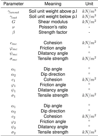
The Strength Factor Beta , which can be computed by equation3.17, relates the dimensions of the single brick with the cohesion. Parameters of the Masonry Model are illustrated in table3.4.

= tan 'b

2a (3.17)

Table 3.4: Parameters of the Masonry Jointed Model.

Parameter Meaning Unit

unsat Soil unit weight above p.l kN/m3 sat Soil unit weight below p.l kN/m3

G Shear modulus kN/m2 ⌫ Poisson’s ratio -Strength factor -cmc Cohesion kN/m2 'mc Friction angle mc Dilatancy angle mc Tensile strength kN/m2 ↵1 Dip angle ↵2 Dip direction c1 Cohesion kN/m2 '1 Friction angle 1 Dilatancy angle 1 Tensile strength kN/m2 ↵1 Dip angle ↵2 Dip direction c2 Cohesion kN/m2 '2 Friction angle 2 Dilatancy angle 2 Tensile strength kN/m2

3.2.2.A Masonry model simulation

In order to characterize the response of the Masonry model a numerical test was carried out using PLAXIS 2D. Two panels, with and without opening were taken into account. The panels are 1 m high and 0, 99 m wide. On the other hand the opening has a dimension of 400x235 mm2_{as can be seen in}

figure3.14. The test was repeated with three different sets of parameters. The first one (set a) presents joints along x direction, the second one (set b) along y direction and the last one (set c) presents a first weak direction with ↵1equals to 45 and a second one with ↵1equals to 135 . These last two dip angles

are chosen in order to simulate the diagonal frontals on the Pombalino masonry wall. Table3.5presents parameters of sets considered. The numerical test carried out in PLAXIS 2D consists in three phases: during the first one zero initial stresses are generated by using the K0 procedure, then during phase 1 a vertical uniform load is applied to the top of the panel and to conclude, during phase 2, a uniform line displacement is applied at the top surface. The calculation type for phase 1 and 2 is set to Plastic. The boundary condition of the bottom surface was set to Normally fixed. The imposed displacement was 1E 6 mand the vertical uniform load was 50 kP a. Ground and upper floors of Pombalino are built with different dimensions stone, therefore to simplify we assumed the same value of height and length for each block(a = b). As a results, the Strength Factor Beta becomes (equation3.18):

= tan '

2 (3.18)

Figure 3.14: Geometry of panels tested. Dimensions are given in meters.

Table 3.5: Parameters of the Masonry Jointed Model for the tests.

Parameter set a set b set c Unit

20 20 20 kN/m3

G 410E3 410E3 410E3 kN/m2

⌫ 0,2 0,2 0,2 -0,445 0,445 0,445 -cmc 90 90 90 kN/m2 'mc 23,98 23,98 23,98 mc 0 0 0 mc 135,00 135,00 135,00 kN/m2 ↵1 0 90 45 ↵2 90 90 90 c1 5 90 5 kN/m2 '1 23,98 23,98 23,98 1 0 0 0 1 7,5 135,00 7,5 kN/m2 ↵1 0 0 135 ↵2 90 90 90 c2 90 10 15 kN/m2 '2 23,98 23,98 23,98 2 0 0 0 2 135,00 15,00 22,5 kN/m2

Deformations "1 and "3 at the end of application of load and horizontal displacements are shown

from figures3.15to 3.20respectively for sets a, b and c. It is noticeable that panels without openings do not suffer of considerable deformations. On the other hand panels with openings present different strains concentrations. For every set of parameters considered "1behaves most as a compressive strain

(negative) and "3as a tensile strain (positive). They both have a magnitude of E 3 with a peak value in

the top right corner of the opening. Sets a and b clearly show a crack pattern which develops according to the weak directions defined by parameter ↵1 and ↵2. Contours of strains "1 and "3 start from the

(a) (b)

Figure 3.15: Total principal strain "1for set a.

(a) (b)

Figure 3.16: Total principal strain "3for set a.

(a) (b)

Figure 3.17: Total principal strain "1for set b.

(a) (b)

Figure 3.18: Total principal strain "3for set b.

(a) (b)

3.3 Drainage conditions simulated in PLAXIS 2D

According to Terzaghi’s principle, stresses in the soil are divided into effective stresses 0 _{and pore}

pressure w:

= 0+ _w (3.19)

Pore pressures are generally provided by water in the pores. Water is considered not to sustain any shear stresses. As a result, effective shear stresses are equal to total shear stresses. Moreover, water is considered to be fully isotropic, so all pore pressure components are equal. Hence, pore pressure can be represented by a single value pw[12].

= 0+ mpactive (3.20) where: m = 2 6 6 6 6 6 6 4 1 1 1 0 0 0 3 7 7 7 7 7 7 5 and pactive= ↵Sepw

where ↵ is Biot’s pore pressure coefficient and Seis the effective degree of saturation. If we consider

incompressible grains, Biot’s coefficient is equal to 1. In PLAXIS 2D ↵Sepw is called ”Active pore

pres-sure”. In addition we can also distinguish between ”Initial pore pressure” pinitialand ”Excess pore stress”

pexcess:

pw= pinitial+ pexcess (3.21)

Initial pore pressures are considered to be input data whereas excess pore pressures are generated during plastic calculations for the case of Undarained (A) or Undrained(B) material behavior or during a consolidation analysis [12].

It is possibile to calculate excess pore pressures. Since the time derivative of the initial component equals zero, it follows:

˙

pw= ˙pexcess (3.22)

By inverting Hooke’s law in terms of total stress and by using undrained parameters Eu and ⌫uit is

possible to evaluate excess pore pressures.

2 6 6 6 6 6 6 4 ˙"e xx ˙"e yy ˙"e zz ˙e xy ˙e yz ˙e zx 3 7 7 7 7 7 7 5 = 1 Eu 2 6 6 6 6 6 6 4 1 ⌫u ⌫u 0 0 0 ⌫u 1 ⌫u 0 0 0 ⌫u ⌫u 1 0 0 0 0 0 0 2 + 2⌫u 0 0 0 0 0 0 2 + 2⌫u 0 0 0 0 0 0 2 + 2⌫u 3 7 7 7 7 7 7 5 2 6 6 6 6 6 6 4 ˙xx ˙yy ˙zz ˙xy ˙yz ˙zx 3 7 7 7 7 7 7 5 (3.23) Where: Eu= 2G(1 + ⌫u) (3.24) ⌫u= 3⌫0_{+ ↵B(1 2⌫}0₎ 3 ↵B(1 2⌫0₎ (3.25)

where B is Skempton’s B-parameter.

B = ↵

↵ + n(_KK_w0 + ↵ 1) (3.26) According to equations (3.24) and (3.25) is possible to transform G and ⌫0 _{into E}

uand ⌫u. In order

to avoid numerical problems caused by an extremely low compressibility ⌫uis by default taken as 0, 495.

Moreover to ensure realistic computational results is considered ⌫0_{< 0, 35[12].}

For material behaviour Undrained(A) or Undrained(B) a bulk modulus for water is automatically con-sidered in the stiffness matrix. Alternately the user can specify the value of the bulk stiffness of water otherwise it is added automatically by the following equation:

Kw

n =

3(⌫u ⌫0)

(1 2⌫u)(1 + ⌫0)

K0 (3.27)

where K0 _{is the effective bulk modulus of the soil matrix and K}

s is the bulk modulus of the solid

material. n is the porosity:

n = e0

3.4 2D Model

In this section the 2D model implemented in PLAXIS 2D is explained in detail. Two different cases were considered with the aim of simulate in a soil deposit displacements due to the decrease of water table.

3.4.1 Ground model

3.4.1.A Geometry

A soil deposit of 25, 0 m thickness is considered. It is composed by three layers (table3.6): the upper layer (ZG1), representative of a backfill, goes from a depth of 0 to 1, 5 m, the middle layer (ZG2), representative of alluvium deposit, goes from 1, 5 to 10 m and the bottom layer (ZG3), representative of miocene deposit, goes from 10 to 15 m. Under ZG3 is situated a stiff rock layer that extends to a large depth and it is not included in the model. The geometry of the model is showed in figure3.21.

The goal is to study displacements and stresses dield caused by the decrease of watertable. To simulate the variation of water level in PLAXIS 2D five different phases were taken into account. At the initial phase the water table is stable at 22 m. During each phase a drawdown of 1 m is considered. At the end of calculation (phase 5) the water table is stable at 17 m.

Table 3.6: Soil layers in Restauradores square.

Layer Depth Thickness (m) (m) ZG1 0 - 1,5 1,5 ZG2 1,5 - 10 8,5 ZG3 10 - 25 15

Figure 3.21: Geometry of the model without underground structure.

3.4.1.B Properties

Hardening Soil with small-strain stiffness model describes well the behaviour of Lisbon downtown soil as studied by Silva [11]. Parameters chosen for the simulation (tables3.7and ) come from the GeoSIS Lx research project promoted by the Municipality of Lisbon. In these simulations, it is assumed that, con-sidering the relatively low permeability of the alluvium soil layer, the water level drawdown occurs at a very low rate, possibly along several years or even decades. To simulate this in a easy manner, without increasing tremendously the computation time, the analysis was performed in drained conditions varying the position of the water level from the initial position to the lowest level.

Table 3.7: Parameters of ZG1 with Mohr Coulomb model.

Parameter Meaning Value Unit Type Drainage type Drained

-unsat Soil unit weight above p.l. 17,6 kN/m3 sat Soil unit weight below p.l. 17,6 kN/m3

E0 _{Young’s modulus (constant) 8,3E3 kN/m}2

⌫0 _{Poisson’s ratio 0,3}

-c0

ref Cohesion 0 kN/m2

Table 3.8: Parameters of ZG2 and ZG3 with Hardening Soil with small-strain stiffness model.

Parameter Meaning ZG2 ZG3 Unit

T ype Drainage type Drained Drained

-unsat Soil unit weight above p.l. 17,6 18,5 kN/m3 sat Soil unit weight below p.l. 17,6 18,5 kN/m3

c0ref (Effective) cohesion 0,00 0,00 kN/m2

'0 _{(Effective) angle of internal friction 29,00 35,00}

Dilatancy angle 0,00 0,00

E50ref Secant stiffness in standard drained triaxial test 125,0E3 250,0E3 kN/m2

E_oedref Tangent stiffness for primary oedometer loading 125,0E3 250,0E3 kN/m2

Eref

ur Unloading / reloading stiffness 145,0E3 750,0E3 kN/m2

m Power for stress-level dependency of stiffness 0,5 0,8

0.7 Shear strain at which Gs= 0.722G0 0,3E-3 1,0E-4

Gref0 Shear modulus at very small strains 145,0E3 300,0E3 kN/m2

⌫0 Poisson’s ratio 0,3 0,25

-kx Horizontal permeability 1,56E-5 1,45E-4 m/day

ky Vertical permeability 1,56E-5 1,45E-4 m/day

type Interface strength type Rigid Rigid

-Rinter Interface strength 1,0 1

-K0determination Manual Manual

-k0,x Lateral earth pressure coefficient 0,5 0,67

-OCR Over-consolidation ratio 1,0 1,0

-P O-P Pre-overburden ratio 0,0 0,0

-3.4.1.C Results

The maximum total displacement at the end of calculation is equal to 2, 975 mm and it is reached at the top surface of the soil deposit as showed in figure3.23. Its horizontal component is negligible, so it develops downward. Figure3.22illustrates the trend of effective vertical and horizontal stresses at the end water drawdown. According to the linear elasticity theory equations3.29and3.30allow to calculate one dimensional settlement for a soil layer:

" = 0

E (3.29)

h = "· h (3.30)

Considering ZG1 which has a thickness of 1, 5 m and a Young’s modulus of 8, 3E3 kP a the settlement calculated results to have a magnitude of mm as computed by PLAXIS 2D.

Figure 3.22: Principal vertical effective stress (blu) and principal horizontal effective stress (orange) at the end of water drawdown.

3.4.2 2D with underground structure

3.4.2.A Geometry

In this case the geometry of soil layers and their parameters are the same of the previous case (tables

3.7and4.3). An underground structure 30 m long and 8 m deep is installed in the center of the model. The side and the base of the structure are supported by diaphragm walls which ensure they are im-pervious. The geometry of the model is showed in figure3.24. To simulate the pumping of water from the excavation, five different phases are taken into account. During each phase a drawdown of 1 m is considered as in the previous case. At the end of phase 5 there is no presence of water at the base of excavation. The drawdown was computed by PLAXIS 2D by creating at each phase a new water table. The shape of water level during drawdown was determined using settlement contours. In conclusion, in order to investigate the effects of a possible drawn up of the water table, a new phase is added. In this phase the water table rises up to the original level (22 m). The shape of water level during water drawdown was determined using settlement contours

Figure 3.24: Geometry of the model with underground structure.

3.4.2.B Properties

Properties of layers ZG1, ZG2 and ZG3 are the same of tables3.7and4.3. In this study the construction of the wall is not taken into account, hence parameters of diaphragm wall were chosen in order to guarantee that it was sufficiently rigid. Table3.9contains parameters of the wall.

Table 3.9: Material properties of the diaphragm wall.

Parameter Name Value Unit

Material type Type Elastic; Isotropic -Normal stiffness EA 12E+06 kN/m

Flexural rigidity EI 1,8E+06 kNm2_/m

Weight w 10,00 kN m2_/m

Poisson’s ratio ⌫ 0,00

-3.4.2.C Results

In order to investigate the effects of water level decrease on displacements at surface the option Reset displacements to zero was selected after the phase of parking area activation. Figures3.26, 3.27and

3.28show trends of displacements at each calculation phase in the surroundings of the parking area, more precisely on the left side of excavation from x = 55, 89 m to x = 67, 74 m. Settlements due to the decrease of water level are correspond to parallel curves that develop gradually upward. Curve installation represents displacements due to the activation of the self weight of the building and curve rise is the curve of settlements induced by the rise of water level.

Figure3.32allows to relate each line displacement to the respective water drawdown. A maximum total displacement corresponding to 2, 64E 3 m is reached at phase 5 when the drawdown is com-pleted. This value is comparable with the maximum displacement obtained after the activation of the parking area, but they follow a different path. Figure3.29illustrates the deformed mesh after the wa-ter drawdown. It exhibits deformations which follow the same trend described by settlements due to the decrease of water level. Moreover figure3.28 shows that settlements due to the rise up of water level (black curve) do not induce remarkable effects. Figure3.31shows a narrow representation of total displacement. It is evident that settlements are influenced by the activation of the parking area and progressively by the water level decrease.

Figure3.32illustrates how water pressure varies consistently with the water table levels assigned in PLAXIS 2D in the Flow condition section. Finally figure3.33is a sequence of shading maps representing the evolution of total displacements. Settlements due to the activation of the parking area develop under the central part of the construction. On the other hand settlements due to the water lowering gather from

Figure 3.25: Evolution of water drawdown surrounding the parking area.

Figure 3.26: Evolution of total displacements surrounding the parking area.

Figure 3.29: Deformed mesh at the end of calculation.

Figure 3.30: Contour lines of total displacements at the end of water drawdown.

(a) (b)

(c) (d)

(e) (f)

Figure 3.33: Evolution of total displacements.

4

Case study

Contents

4.1 Modeling Pombalino facade . . . 57

4.2 Drawdown of water level . . . 61

4.3 Results . . . 63

In this chapter is presented the case study of a Pombalino edge located 2 m far from an excavation. Pombalino building and soil models are described in detail in the following section.

4.1 Modeling Pombalino facade

4.1.1 Geometry of Pombalino facade

The Pombalino building chosen was characterized by Renda [6], therefore a large amount of data is available. The building simulated extends horizontally for 17, 96 m and it has a total height of 15 m from the surface. It presents a ground floor 4, 5 m high and three upper floors with an height of 3, 5 m each. Each floor has six parallel openings with different dimensions. The foundation system simulated is made by a slab of 1 m thick and seven timber piles 2 m long. The ground floor and the foundation system consist of walls and columns in stone masonry. The upper floors are built in ordinary masonry. Figure

4.1illustrates the geometry of the facade simulated. It is possibile to note the main differences with the real facade of Pombalino building as the absence of roof and wooden piles.

Figure 4.1: Geometry of the real Pombalino building studied (left), and building simulated in PLAXIS 2D (right).

4.1.2 Properties of Pombalino facade

In PLAXIS 2D Pombalino building was simulated with two different material models: foundations and ground floors with Mohr-Coulomb model, externals upper walls with Masonry Model, in which an horizon-tal weak direction is selected in order to take into account the orientation of laying stones. In Pombalino buildings frontal timber crosses were installed about 200 years ago to respond to earthquake motion, but now they are particularly degraded, especially at the connections. They became weak directions that cross each other with a dip angle of 45 and 135 (figure4.2). The area between frontals is filled by masonry built by stones with smaller dimensions than the ones of the ground floor. In order to reproduce this constructive elements a Masonry model was assigned to the openings and two joint families were selected and oriented as the wooden frontals. The same value of height and length was considered for each masonry block (a = b), therefore is expressed by equation3.18, due to the randomness of the size and orientation of ordinary masonry.

Parameters of ground floor, slab and piles are presented in table4.1. Their values are provided by the Italian regulations NTC 2008 applying the drawdown factor of 50 % for Young modulus and shear modulus. Parameters of upper floors were obtained thanks to experimental works developed by Santos (1997) in old buildings that were later demolished [6]. These latter are contained in table4.2.

Table 4.1: Parameters of Pombalino building foundations and ground floor.

Parameter Value Unit

Material Model Mohr-Coulomb Model

22 kN/m3 G 430E3 kN/m2 E0 1,032E6 kN/m2 ⌫0 0,2 -c0ref 140 kN/m2 '0 _23,98 0

Table 4.2: Parameters of Pombalino building upper floors.

Parameter Value Unit Material Model Masonry Model

20 kN/m3 G 410E3 kN/m2 ⌫ 0,2 -0,445 -cmc 90 kN/m2 'mc 23,98 mc 0 mc 135,00 kN/m2 ↵1 0 ↵2 90 c1 5 kN/m2 '1 23,98 1 0 1 7,5 kN/m2

4.1.3 Soil profile

The soil deposit considered consists of three layers with a total thickness of 25, 0 m. The upper layer (ZG1) representative of a fill and goes from a depth of 0 to 1, 5 m. The middle layer (ZG2) is the alluvium layer and goes from 1, 5 to 10 m. The bottom layer (ZG3) is the miocene layer and goes from 10to 15 m. Under ZG3 is situated a vey stiff soil layer that extends to a large depth and it is not included in the model. The excavation is carried out from 70 to 100 m up to a depth of 17 m. Pombalino is located 2 mfar from one side of the excavation. Figures4.3and4.4show respectively the geometry of the case study and the mesh generated by PLAXIS 2D. This latter is created with the command fine elements

and it is composed by 1540 soil elements and 12685 nodes. The average element size is 2, 168 m, the maximum 8, 009 m and the minimum 0, 5 m.

4.1.4 Soil properties

Parameters of soil layers are the same of study cases developed in chapter3and they are presented in tables3.7and4.3. Also parameters of diaphragm wall are the same of previous case (table3.9). In PLAXIS 2D the layer ZG1 was modeled with a Mohr-Coulomb model because the deformation in this layer is not so relevant for the global response of the model. On the other hand the Hardening Soil with small-strain stiffness model was used for ZG2 and ZG3. This numerical model can simulate more accurately stiffness in the small strain range. In our case study the water level drawdown induces small to moderate stress variation, so it is important to simulate well the small strain stiffness. Hardening Soil with small-strain stiffness model requires to define for each layer two additional parameters which describe the behaviour of stiffness in the range of small deformations (G0) and the rate of stiffness

degradation ( 0.7). With equation4.1is possible to compute the maximum shear modulus G0:

G0= ⇢· Vs2 (4.1)

where:

⇢ =

g (4.2)

Knowing values of for layers ZG2 and ZG3 is possible to obtain values of G0 and the Young

modulus through equation4.3:

E = 2G(1 + ⌫) (4.3)

Finally equation 3.8 was implemented to compute the stiffness degradation curve. The value of deformations corresponding to G/G0= 0, 7is the second additional parameter needed in the HS small

model.

4.2 Drawdown of water level

Pombalino building is a structure built after the earthquake of 1755. In the early 1990’s, several exca-vations to install underground parking area were done in Baixa, with pumping systems active during construction and on service. Only the water level drawdown is considered. In other words the action of the pumping system used to drawdown water table is simulated by drawing a new water level at each phase and by assuming it as the new Global Water Table. As explained in chapter 2, the monitoring campaign performed on request of the Municipality of Lisbon extended from 2004 to 2010. Thus this thesis intends to characterize the impact of water table drawdown on surface displacements and if this settlements can explain the damage pattern observed in Pombalino buildings. Moreover, in order to in-vestigate the effect of the rise of water table, another phase in which water level increases is considered.

Table 4.3: Parameters of ZG2 and ZG3 with Hardening Soil with small-strain stiffness model.

Parameter Meaning ZG2 ZG3 Unit

T ype Drainage type Drained Drained

-unsat Soil unit weight above p.l. 17,6 18,5 kN/m3 sat Soil unit weight below p.l. 17,6 18,5 kN/m3

c0ref (Effective) cohesion 0,00 0,00 kN/m2

'0 _{(Effective) angle of internal friction 29,00 35,00}

Dilatancy angle 0,00 0,00

E50ref Secant stiffness in standard drained triaxial test 125,0E3 250,0E3 kN/m2

E_oedref Tangent stiffness for primary oedometer loading 125,0E3 250,0E3 kN/m2

Eref

ur Unloading / reloading stiffness 145,0E3 750,0E3 kN/m2

m Power for stress-level dependency of stiffness 0,5 0,8

0.7 Shear strain at which Gs= 0.722G0 0,3E-3 1,0E-4

Gref0 Shear modulus at very small strains 145,0E3 300,0E3 kN/m2

⌫0 Poisson’s ratio 0,3 0,25

-kx Horizontal permeability 1,56E-5 1,45E-4 m/day

ky Vertical permeability 1,56E-5 1,45E-4 m/day

type Interface strength type Rigid Rigid

-Rinter Interface strength 1,0 1

-K0determination Manual Manual

-k0,x Lateral earth pressure coefficient 0,5 0,67

-OCR Over-consolidation ratio 1,0 1,0

-P O-P Pre-overburden ratio 0,0 0,0

-In PLAXIS 2D the first calculation stage is set to K0 procedure. Pombalino and the excavation are simultaneously activated from the beginning. During phase 1 the water table is stable and the effects of the installation of Pombalino and excavation are taken into account. From phase 2 to phase 6, five water table decreases of 1 m each occur in the area excavated. The water depression cone simulated in PLAXIS 2D is drawn linearly with the command New water level. Boundary conditions are set to free for Ymax, fixed for Ymin, Xmax and Xmin.