Monitoring and modeling fluxes transfer processes in soil-plant-atmosphere continuum across scales

(1)

UNIVERSITÀ DEGLI STUDI DI CATANIA

INTERNATIONAL PHD COURSE IN

“AGRICULTURE, FOOD AND ENVIRONMENTAL SCIENCE” XXIX CYCLE

Monitoring and modeling fluxes transfer processes in soil-plant-atmosphere continuum across scales

Daniela Vanella

Advisor:

Prof. Simona Consoli Coordinator:

Prof. Cherubino Leonardi

(2)

(3)

Table of contents

i

List of figures

Figure 1.1 A schematic of the critical zone (CZ) components (modified

from Wilding & Lin, 2006; Du & Zhou, 2009)... 2

Figure 1.2 Water balance at the plant scale ... 4 Figure 1.3 Comparison between the number of publications including

‘root water uptake’ and ‘evapotranspiration’ within 1939 and 2015 from Scopus (data not normalized respect to the total number of publications) ... 5

Figure 1.4 Soil moisture measurements obtained by ground-based

sensors and contact-free techniques (modified from Vereecken et al., 2008) ... 10

Figure 1.5 Conceptual model of the hydro-geophysics application (Rubin

and Hubbard, 2005, Vereecken et al., 2006, Binley et al., 2011) ... 11

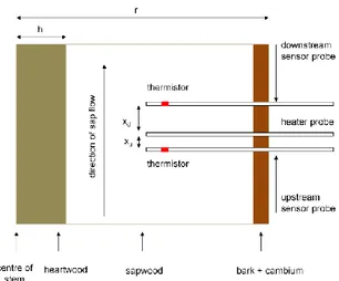
Figure 2.1 Configuration of a single set of heat-pulse probes implanted

radially into a stem (modified from Smith & Allen, 1996) ... 35

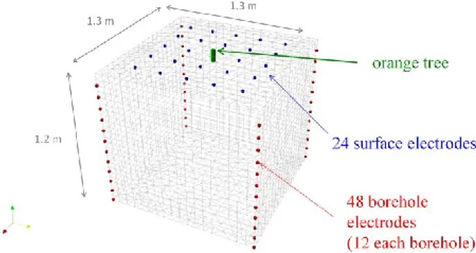
Figure 3.2 Electrode geometry around the orange tree and 3-D mesh

used for ERT inversion ... 45

Figure 3.3 EC micrometeorological equipment at Case study 1. EC tower

(a, b); 3D sonic anemometer, gas analyzer and fine wire thermocouples (c); infra-red remote temperature sensor (d); temperature and relative humidity probe (e); net radiometer (f); sap flow sensors (g, h, i); TDR probes (l); anemometer (m) ... 48

(7)

List of figures

v

Figure 3.5 Cross sections of the ERT cube corresponding to the

background acquisition (initial conditions) (from Cassiani et al., 2015) ... 51

Figure 3.6 Hourly transpiration by sap flow (black line) and ET by EC

(blue lines) fluxes measured at Case study 1, (a). 3-D ERT images of resistivity change with respect to background at selected time instants 52

Figure 3.7 Lab-experimental relationships between electrical resistivity

and soil moisture of samples (a) collected at 0.4 m (b) and 0.6 m (c) below the ground at Case study 1 site ... 54

Figure 3.8 Conceptual 1-D Richards’ equation model (a); results of 1-D

Richards’ equation simulations (b); the area that allows one to match the observed real profile with good accuracy (c) (modified from Cassiani et al., 2015) ... 58

Figure 3.9 Hourly soil moisture from three TDR probes located about

1.5m from the ERT-monitored tree (from Cassiani et al., 2015) ... 60

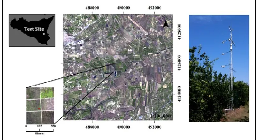
Figure 4.1 Location of the experimental site in Sicily (Italy) (a);

experimental orange orchard (b); orange trees at the study site (c) ... 64

Figure 4.2 Irrigation treatments (T1, full irrigation and T4, PRD) at the

experimental field. The blue circles identify the small scale 3-D ERT installations ... 67

Figure 4.3 Small scale 3-D ERT monitoring scheme for T1 (a) and T4 (b)

treatments. The orange circle represents the trees trunks falling in the quarters C4 and Q4; the black points are the superficial and buried electrodes; the blue dot lines indicate the irrigation pipelines in T1 (a) and T4 (b) treatments ... 71

(8)

List of figures

vi

Figure 4.4 Daily evolution of soil water content (SWC, m3_m-3_{) measured}

by TDR in the PRD (T4) and the control treatment (T1) during the irrigation season 2015 ... 76

Figure 4.5 Hourly soil water content (SWC, m3_m-3_{) measured by TDRs}

during the 3-D ERT monitoring in 2015: June, ERT1 (a), July, ERT2 (b), September, ERT3 (c) ... 78

Figure 4.6 (previous page) Absolute inversions of the background

datasets collected during the long-term ERT monitoring (ERT1, ERT2, ERT3, June-September 2015), in T1 (a) and T4 (b) treatments. Average resistivity values are reported in function of the depth (c, d) ... 85

Figure 4.7 Box-plots of the electrical resistivity distribution in the

different soil layers in T1 and T4 ... 85

Figure 4.8 (next page) Time-lapse resistivity ratio in T1 and T4 during

July (ERT2, panels a, c) and September (ERT3, panels b, d) respect to the corresponding background conditions ... 89

Figure 4.9 Time-lapse resistivity ratio volume at a selected time step

(after the end of the irrigation, time 03) with respect to the background condition (before irrigation, time 00), a); Tree transpiration rate (mm h-1_),

irrigation and ERT surveys timing are displayed in the graph in function of time, b). Data refers to the full-irrigated treatment (T1) on July 15, 2015 ... 92

Figure 4.10 Time-lapse resistivity ratio volume at a selected time step

(after the end of the irrigation, time 03) with respect to the background condition (before irrigation, time 00), a); Tree transpiration rate (mm h-1_),

irrigation and ERT surveys timing are displayed in the graph in function of time, b). Data refers to the PRD treatment (T4) on September 24, 2015 ... 93

(9)

List of figures

(10)

List of tables

viii

List of tables

Table 2.1 Potential agricultural applications for resistivity (ER),

electromagnetic induction (EM), and ground-penetrating radar methods (GPR) (modified from Allred et al., 2008) ... 16

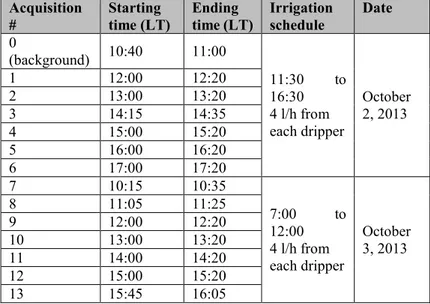
Table 3.1 Times of acquisitions and irrigation schedule ... 44 Table 4.1 Summary of the performances of the total absolute inversion

for ERT1 (a), ERT2 (b) and ERT3 (c) for both the treatments (T1 and T4), for absolute inversion error at 16%. ... 83

(11)

Abbreviations and symbols

ix

Abbreviations and symbols

°C Celsius degree 1D one-dimensional 3D three-dimensional   regularization parameter

’ constants in the water retention van Genuchten model (1980)

a correction coefficient derived by Swanson and Whitfield (1981)

ACM Citrus and Mediterranean Crops Research Centre b correction coefficient derived by Swanson and

Whitfield (1981)

c correction coefficient derived by Swanson and Whitfield (1981)

c’ scalar concentration fluctuations C1 first quarter treatment T1 C2 second quarter treatment T1 C3 third quarter treatment T1 C4 fourth quarter treatment T1

CREA Italian Council for Agricultural Research and Agricultural Economics Analyses

cp specific heat of air at a constant pressure

CZ critical zone

d data (measured apparent resistivity) di measurement data vector

dr resistance ratio

d0 dataset collect at the initial condition

dt data collected at time (t)

DC direct current DT  displacement of water   data error m parameter update T temperature variation EC eddy covariance

(12)

x

EM electromagnetic induction ER electrical resistivity

ERT electrical resistivity tomography ERT1 first ERT monitoring 2015 ERT2 second ERT monitoring 2015 ERT3 third ERT monitoring 2015 ET0 reference evapotranspiration

ET evapotranspiration

FDR frequency domain reflectometry Fm forward model

FM volume fractions of wood

FL volume fractions of water

G soil heat flux

GPR ground-penetrating radar H sensible heat flux h radius

hc canopy height

HPV heat pulse velocity

J Jacobian (or sensitivity) matrix j sap flux density

k iteration K geometric factor

K(h) soil hydraulic conductivity tensor Kc crop coefficient

Ks hydraulic conductivity at saturation

λ latent heat of vaporization λE latent heat flux

LAI leaf area index LT local time m model parameter

m’ constants in the water retention van Genuchten model (1980)

MD mass of dry wood

MF mass of fresh wood

ML mass of water

n constants in the water retention van Genuchten model (1980)

(13)

xi

N number of measurements PAR photosynthetic active radiation pF retention curve

PRD partial root-zone drying

q’ concentration of the transported water vapour Q1 first quarter treatment T4

Q2 second quarter treatment T4 Q3 third quarter treatment T4 Q4 fourth quarter treatment T4

SIAS Agro-meteorological Service of the Sicilian Region

SP soil-plant

SPAC soil-plant-atmosphere continuum SWC soil water content

a apparent resistivity

m calculated resistivity

air air density

 electrical resistivity L water density

M density of dry wood

R roughness matrix r stem radius

RMS root mean square misfit RN net radiation

RS remote sensing RWU root water uptake S sink source term

  volumetric soil water content r  residual water content

s  saturated water content

t time

T temperature

T1 full irrigation treatment T4 deficit irrigation treatment TDR time-domain reflectometry TSF transpiration

(14)

xii

Vc corrected heat pulse velocity

VT total volume

Vz raw heat pulse velocity

w’ vertical velocity fluctuations Wd data weight matrix

WPL Webb, Pearman, Leuning

Xu upstream distance below the heater

Xd downstream distance above the heater

d objective function

(15)

Acknowledgements

xiii

Acknowledgements

The pages of this manuscript are the work of many minds and hands that I have been lucky to meet during the PhD years. My best thanks are to my Advisor – prof. Simona Consoli - for all the guidance and opportunities that she gave me during the PhD period.

I wish to thank the components of hydraulic research group of the Department of Agriculture, Food and Environment (DI3A), University of Catania - prof. Salvatore Barbagallo, prof. Giuseppe Cirelli, dr. Rosa Aiello, dr. Feliciana Licciardello - for welcoming me into a “research family”. I really thank the members of geophysics research group of the Department of Geoscience, Padua University - prof. Giorgio Cassiani, dr. Jacopo Boaga, dr. Maria Teresa Perri, dr. Laura Busato - for the intense collaboration that we have built in these years, their huge assistance in the geophysical experimental design.

I am sincerely grateful to prof. Andrew Binley for the precious teachings and recommendation on the use of hydro-geophysics techniques and for his twice hospitality at the Lancaster Environment Centre (LEC) of Lancaster University (UK).

I wish to thank dr. Giovanni Zocco and dr. Alessandro Castorina for their help during the geophysical monitoring fieldwork in 2015.

(16)

Acknowledgements

xiv

Moreover, I wish to thank the personnel of the Citrus and Mediterranean Crops Research Centre of the Italian Council for Agricultural Research and Agricultural Economics Analyses (CREA-ACM, Acireale) and especially dr. Giancarlo Roccuzzo and dr. Fiorella Stagno for their support in the research activity.

Without the help of all these people, this thesis would never have come into existence. Now I wish you an enjoyable travel through the pages of this manuscript.

(17)

Preface

xv

Preface

Complex exchange processes characterize the soil, vegetation and the lower atmosphere system. While the exchange of mass (mainly water and carbon) and energy is continuous between these compartments, the pertinent transfer fluxes are strongly heterogeneous and variable in space and time. Within the soil-plant-atmosphere continuum (SPAC) system, root activity plays a crucial role because it connects different domains and allows the necessary water and nutrient exchanges for plant growth. Plant roots have a major role in mass and energy exchanges between soil and atmosphere. Yet, monitoring the activity of the root-zone is a challenge as roots are not visible from the soil surface and they evolve in space and time responding to internal and external forcing conditions. Therefore, devising strategies that can provide insight into the activity of roots have an impact both on practical activities such as precision agriculture and on answering large-scale questions e.g. related to climatic change.

The comprehension of the mass exchange dynamics within the SPAC is useful not only for eco-hydrological purposes, by contributing to the understanding of the critical zone (CZ) dynamics (Jayawickrem et al., 2014; Parsekian et al., 2015), but also plays a central role in the definition of precision agriculture criteria, especially when an optimisation of water resources exploitation is mandatory.

(18)

Preface

xvi

The PhD thesis is organized into five Chapters.

The first Chapter contains both an introduction on the general concepts, based on the research motivations, and a summary of the main objectives of the PhD work.

The second Chapter presents a theoretical insight on the methodological approaches adopted during the experimental campaigns.

The third and fourth Chapters systematically describe two experimental Case study applications. Each of these Chapters includes a description of the field site and the materials and methods, the achieved results and discussions.

(19)

Abstract

xvii

Abstract

The soil-plant-atmosphere (SPA) interactions are a critical component of the Earth's biosphere because of their crucial role in the hydrological cycle. For a better understanding of the functional interactions between natural resources and related sustainability problems, the scientific community is becoming aware that more interdisciplinary approaches are required.

Understanding SPA processes and principally root-zone uptake (RWU) is actually significant for proper irrigation management especially in areas characterized by scarce water availability, such as the Mediterranean areas. Such understanding requires an ability to map the hydrological dynamics at high spatial and temporal resolution and appropriate scale.

The PhD work encourage at using innovative and advanced techniques to monitor the exchanges of mass and energy within the soil-plant-atmosphere continuum (SPAC) at different spatial scales.

The novelty of the PhD work is the assimilation of geophysical data with other more conventional measurements (micrometeorogical and transpiration data) in order to interpret some of the principal transfer processes acting through the SPAC (i.e., evapotranspiration and RWU) in semi-arid climate.

(20)

Abstract

xviii

The PhD thesis covers two cases studies looking at the use of an integrated approach to help unravel the complexity of soil-plant interactions, specifically concerning RWU of citrus trees.

In the first Case study, electrical imaging, sap flow data, eddy covariance measurements and modelling were coupled to determine the RWU area of an orange tree.

The second Case study, explores RWU patterns of orange trees under different irrigation schedules, by integrating small scale 3D electrical resistivity tomography (ERT) with sap flow measurements.

Results have demonstrated the ability of electrical imaging techniques to link the soil moisture distribution with crop physiological response (i.e. transpiration fluxes) and the active root distribution in the soil, thus providing new insight into the use of geophysical measurements.

(21)

Sommario

xix

Sommario

Alle interazioni tra le diverse componenti del sistema suolo-pianta-atmosfera (SPA) è attribuito un ruolo critico nel ciclo idrologico e della biosfera terrestre.

La comunità scientifica specializzata è sempre più consapevole della necessità di portare avanti studi a carattere interdisciplinare per la comprensione delle interazioni funzionali tra le risorse naturali ed i relativi problemi di sostenibilità del sistema SPA.

All’interno di tali studi interdisciplinari, l’analisi delle interazioni suolo-radice risulta rilevante anche per la gestione ottimale dell'irrigazione, in particolare nelle zone caratterizzate da scarsa disponibilità idrica, come le aree mediterranee. A tal fine nasce l’esigenza di valutare, ad alta risoluzione sia spaziale che temporale, le dinamiche idrologiche del sistema SPA, sino alla scala dell’apparato radicale.

Il contributo della tesi di dottorato consiste nell’applicazione di tecniche di monitoraggio avanzate e minimamente invasive, per valutare gli scambi di massa ed energia all'interno del sistema SPA.

L’aspetto innovativo del lavoro di tesi consiste nell’integrazione di tecniche geofisiche con misure micrometeorologiche e dati di traspirazione, al fine di interpretare alcuni dei principali processi di trasferimento di

(22)

Sommario

xx

flussi nel sistema SPA (evapotraspirazione ed assorbimento radicale) in ambiente semi-arido.

Tale approccio, è stato applicato a due Casi studio con l’obiettivo di monitorare le complesse interazioni del sistema suolo-pianta, con particolare riferimento al processo di assorbimento radicale di alberi di agrume.

Nel primo Caso studio, la tecnica della tomografia di resistività elettrica (ERT) tridimensionale è stata integrata con dati di traspirazione, misure micrometeorologiche e modellistica idrologica al fine di delineare la porzione di suolo non satura interessata dalle radici attive di un aranceto adulto.

Nel secondo Caso studio, il monitoraggio ERT è stato integrato con misure di traspirazione al fine di delineare i pattern di RWU di alberi di arancio irrigati in regime di deficit.

I risultati del lavoro di tesi dimostrano l’abilità della tecnica di monitoraggio geofisico ERT nello spiegare le dinamiche idriche del suolo e la risposta fisiologica della pianta, in termini di attività delle radici nel processo di uptake, contribuendo, in tal senso, a migliorare la conoscenza dei processi di assorbimento radicale.

(23)

Chapter 1. Introduction

1

Chapter 1

(24)

2

Introduction

1.1 The soil-plant-atmosphere relationship

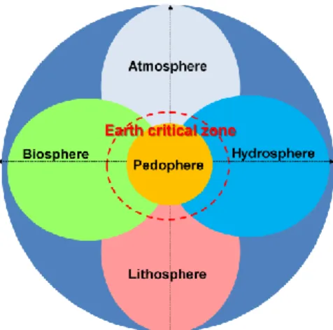
The “critical zone” (CZ) is the breathing skin of Earth: a life-supporting epidermis that reaches from the top of vegetation down through soil and bedrock (Parsekian et al., 2015). Starting from this definition, soil and water are two critical components of the Earth’s CZ. A schematic of CZ components is given in Figure 1.1.

Figure 1.1 A schematic of the critical zone (CZ) components

(25)

3

In general, soil modulates the connection between bedrock and atmospheric boundary layer and water is a major driving force and transport agent between these two compartments. The interactions between soil and water are so close and complex that cannot be effectively studied by stand-alone approaches. They require a system approach. The pedosphere as defined by Du & Zhou, (2009) is the thin skin of soil on the Earth’s surface that represents a geomembrane across which water and solutes, as well as energy, gases, solids, and organisms are actively exchanged with the atmosphere, biosphere, hydrosphere, and lithosphere to create a life-sustaining environment. Soil–water interactions create the fundamental interface between the biotic and abiotic and hence serve as a critical determinant of the state of the Earth system and its critical zone (Wilding & Lin, 2006).

In recent years, authors (Lin, 2010 and references inside) have demonstrated that interdisciplinary approaches have significance in advancing both soil science and hydrology and can guide more effective field data acquisition, knowledge sharing, model-based prediction of complex scenario and soil-plant-atmosphere continuum (SPAC) relationships across scales. John R. Philip pioneered the concept of SPAC, as follows: "Because water is generally free to move across the soil, soil-atmosphere, and plant-atmosphere interfaces it is necessary and desirable to view the water transfer system in the three domains of soil, plant, and atmosphere as a whole ...it must be pointed out that, as well as serving as a vehicle for water transfer, the SPAC is also a region of energy transfer" (Philip, 1966).

(26)

4

In this spirit, the synergistic integration of soil and life science in combination with hydrology can offer a renewed perspective and an integrated approach to understanding interactive soil and water processes and their properties in the CZ (Lin et al., 2015; Lin et al., 2003). As expected from the above description, the unsaturated soil is a complex system governed by greater non-linear processes and interactions. The SPAC systems that cover the lands of our Earth are the Earth’s CZs, providing valuable ecosystem services (NRC, 2004). Through these systems, there are massive fluxes and storages of mass (water and carbon) and energy, and these provide both valuable productive and ecosystem goods and services.

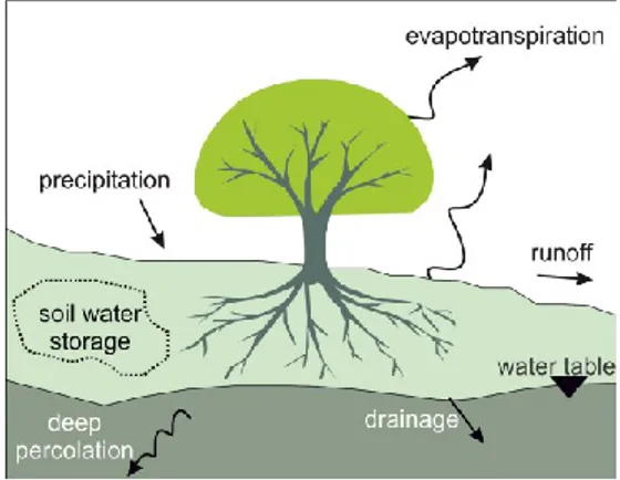
Figure 1.2 Water balance at the plant scale

Progress has achieved in advancing scientific knowledge on the SPAC and understanding the controls on hydrologic fluxes as well as how these controls vary spatially and temporally with scale (e.g., Cammalleri et al., 2013; Cassiani

(27)

5

et al., 2015; Consoli & Vanella, 2014 a and b; Minacapilli et al., 2016). At larger scale, crops affect the terrestrial water cycle and underground water dynamics through evapotranspiration (ET) and root water uptake (RWU), respectively. An overview of the principal hydrological processes acting within the SPAC at the small scale is shown in Figure 1.2. It is therefore not surprising that the understanding of water flow processes taking place in the SPAC has been a popular research topic during the second half of the 20th_{and beginning of the 21}st_century.

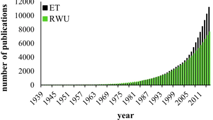
Figure 1.3 Comparison between the number of publications

including ‘root water uptake’ and ‘evapotranspiration’ within 1939 and 2015 from Scopus (data not normalized respect to the total number of publications)

The graph in Figure 1.3 reports a comparison between the number of publications with title, abstract or key words containing ‘root water uptake’ and ‘evapotranspiration’ within 1939 and 2015, limiting the search to the “agriculture”

0 2000 4000 6000 8000 10000 12000 nu m ber of pu bli ca tio ns year ET RWU

(28)

6

subject area (Source: Scopus, https://www.scopus.com). At the end of the year 2015 the publications containing the words “evapotranspiration” or “root water uptake”, with the characteristics described above, were 11191 and 7667, respectively; with an increment of about 65 and 53% in last ten years, respectively.

1.2 Root water uptake models

In this paragraph, there is a summary on the state-of-the-art about modelling and estimates of root water uptake (RWU). The translation of water use strategies by crops into physically based models of RWU is a crucial issue in eco-hydrology and no agreement exists on the modelling of this process (Feddes et al., 2001; Raats, 2007). The mechanisms of water transport within unsaturated soil layers in the root-zone are mainly controlled by soil physics, plant physiology and meteorological factors (Green et al., 2003a). Today there is a general accord on the tension-cohesion theory to describe the ascent of water in plants. This theory states that the water is passively extracted from the soil and flows to the atmosphere through the plant. The "catenary hypothesis" (van den Honert, 1948) is largely considered as a valid concept to modelling water flow in roots. Water is transported within the SPAC that is principally controlled by the resistances as determined by the rhizosphere, the cortex, the xylem and between the leaves and the atmosphere through the stomata. Resistances in SPAC are generally a function of the plant basic anatomy, development and metabolism; and they are all potentially variable in time and space (Hose et al., 2000;

(29)

7

Carminati and Vetterlein, 2012). Some resistances such as those stomata are also variable depending on plant responses and environmental effects (Blum, 2011). Therefore, the quantification of resistances to water flow along the pathway between the plant and the atmosphere is still the subject of extensive researches. Javaux et al., (2013) report that nowadays measurements of local resistances are still hardly achievable or their determination is still prone to large uncertainty. The uncertainty concerning the magnitude and location of resistances led in the past to simplifying sometimes-simplistic modelling approaches for RWU. Typically, RWU is accounted for the Richards' equation with a sink source term, S [L3_L-3_T-1_]:





S z h t         K(h) K(h) (1.1)

where θ denotes the volumetric soil water content [L3_L-3_{], t}

the time [T], z the vertical coordinate [L], K(h) the soil hydraulic conductivity tensor [L T-1_{]. In the right-hand of the}

Eq (1.1), the two terms describe the water flow redistribution between layers or soil locations, while the third one describes the water uptake by plant roots (S<0) or root exudation (S>0). From a conceptual point of view, two main approaches exist today to predict the volumetric rate of RWU in volume elements of soil (Javaux et al., 2013). On the one hand, physically based models may explicitly consider the three-dimensional distribution of the root system together with a

(30)

8

distribution of the system conductances at plant scale (Doussan et al., 2006; Schneider et al., 2010).

The major limitation of this kind of models is the cost for characterizing parameters, such as root system architecture, conductance to water flow, etc, and the fact that it is very demanding in terms of computational power and time. On the other hand, effective models exist that represent the uptake behaviour at the plant scale through "macroscopic parameters". In the macroscopic approach, the sink term is typically composed of four terms that affect the magnitude and spatiotemporal dynamics of RWU, such as:

 the root hydraulic resistance distribution;  the soil hydraulic resistance;

 a stress function describing the plant answer to an excessive climatic demand of water;

 a compensation function (Jarvis, 1989) representing the impact of the water potential distribution inside plant xylem vessels for the distribution of water uptake from the soil profile.

In three-dimensional models, the two first variables are explicitly considering accounting for the distribution on the root architecture and the root and hydraulic proprieties (potentially changing in time). The third variable is defined by a function of the water potential in the leaf. The fourth variable arises from the solution of the flow equations that are coupled between the root and the soil systems. These functions are usually simple, with few parameters and easy to

(31)

9

compute, but some of their parameters need calibration, which introduces uncertainties (Musters and Bouten, 2000). The RWU modelling complexity is highly related to the irregular root distribution in the vertical and radial directions (Gong et al., 2006). This variability is also induced by uneven soil layers, water and nutrient distribution and the localized soil compaction, caused by both cultivation patterns and frequent irrigation (Jones and Tardieu, 1998).

Therefore, it is evident the need to continue the development of RWU modelling approaches by increasingly the accuracy and completeness of the existing approaches (Feddes et al., 2001; Raats, 2007; Jarvis, 2011; Couvreur et al., 2012), and also integrating them with highly accurate measurements techniques of RWU activity proxy such as monitoring of soil moisture in the root-zone.

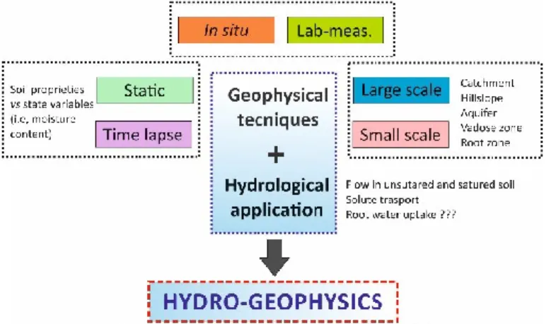
1.3 Hydro-geophysics approach

As introduced above, soil moisture measurements (Figure 1.4) may be paramount to implement RWU models. Traditionally beneath irrigated crops, soil moisture measurements have been determined using point or local measurement methods (Romano, 2014). There are numerous well-accepted methods for measuring soil moisture such as: gravimetric technique, dielectric methods (e.g., time-domain reflectometry, TDR; frequency-domain reflectometry, FDR), capacitance probe, neutron probe techniques.

The advantage of these methods is their robustness, but obviously, they suffer of limited spatial coverage. It is often

(32)

10

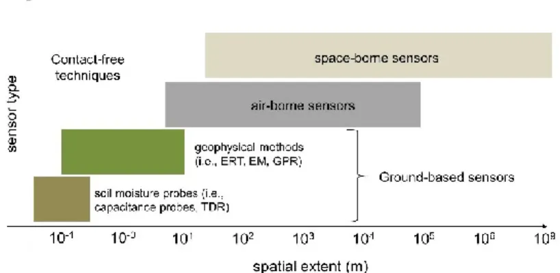
impractical obtain the number of measurements necessary to achieve a good spatial resolution. Furthermore, most of the traditional techniques are invasive and may disturb the in situ moisture distribution that is required from the measurement. Robinson et al. (2008) report that contact free measurement techniques, such as remote sensing (RS) methods including passive microwave radiometers, are prominent in this category. These approaches are either ground based or operated from airborne or space borne platforms. Key limitations of current RS methods are problems with spatial averaging and a small penetration depth.

Figure 1.4 Soil moisture measurements obtained by

ground-based sensors and contact-free techniques (modified from Vereecken et al., 2008)

Contact-free hydro-geophysical methods are also increasingly used (Vereecken et al., 2008). The past twenty years, in particular, have seen the fast development of geophysical techniques that are useful in identifying structure

(33)

11

and dynamics of the near surface, such as soil moisture distribution, with particular reference to hydrological applications. This realm of research goes under the general name of hydro-geophysics (Rubin et Hubbard, 2005, Vereecken et al., 2006, Binley et al., 2011; Binley et al., 2015a) and covers a wide range of applications and different spatial scales, from flow and transport in aquifers (e.g.,. Kemna et al., 2002; Perri et al., 2012) to the vadose zone (e.g. Daily et al., 1992, Müller et al., 2010; Oberdörster et al., 2010) (Figure 1.5).

Figure 1.5 Conceptual model of the hydro-geophysics

application (Rubin and Hubbard, 2005, Vereecken et al., 2006, Binley et al., 2011)

Authors have demonstrated how especially electrical geophysical methods can successfully image moisture dynamics in both field and laboratory (Koestel et al., 2008) settings. These methods can provide spatially continuous

(34)

12

information, thus avoiding the need for interpolation between sparsely distributed point-based measurements. For example, moisture fronts following natural rainfall events have been imaged by electrical resistivity imaging (Zhou, ey al., 2001; Binley et al., 2002; Robinson et al., 2012a; Schwartz et al.,2008), supported by laboratory experiments to determine appropriate pedophysical relationships to convert resistivity changes to changes in the distribution of moisture content. Such studies have conclusively demonstrated that surface-electrical resistivity is a viable method for monitoring and defining vadose zone transport parameters and redistribution processes (Robinson et al., 2012). Generally, electrical resistivity can be related to soil state variables (such as soil moisture and salt concentration) and properties (clay content) and as well root properties, such as root mass (Amato et al., 2008; Paglis, 2013; Rossi et al. 2011).

Time-lapse geophysical measurements may be used to monitor spatial patterns of dynamic processes like water flow, root water uptake, and/or solute transport in soils in agricultural contexts (for details see, paragraph 2.1).

Relatively numerous hydro-geophysical applications, though, have been focussed on plant root system characterization (e.g. al Hagrey, 2007; al Hagrey and Petersen, 2011; Javaux et al., 2008; Jayawickreme et al., 2008; Werban et al., 2008), often limiting the analysis to a tentative identification of the main root location and extent. As mentioned above, electrical soil properties are a clear indication of soil moisture content distribution, and electrical

(35)

13

and electromagnetic methods have been used to identify the effect of root activity (e.g. Cassiani et al., 2012; Shanahan et al., 2015). In particular, electrical resistivity tomography (ERT) has been used to characterize RWU and root systems (Garré et al., 2011; Michot et al., 2001, 2003; Srayeddin and Doussan, 2009). Amato et al. (2009, 2010) tested the ability of 3-D ERT for quantifying root biomass on herbaceous plants. Beff et al. (2013) used 3-D ERT for monitoring soil water content in a maize field during late growing seasons. Boaga et al. (2013) and Cassiani et al. (2015) demonstrated the reliability of the method respectively in apple and orange orchards. These works provide useful and promising insights into the application of the hydro-geophysical approach for the SP system characterization.

1.4 Objectives

The main objectives of the PhD work are: (i) to evaluate a new approach to understanding SPAC dynamics across space and time and (ii) to explore synergistic efforts from soil science and hydrology, along with other related disciplines such as hydro-geophysics, micrometeorology and life science.

Herein, different methodologies were coupled (e.g., geophysical methods, sap flow techniques, micro-meteorological approaches) with the main purpose of improve our understanding on the effect of soil-root interface on water dynamics.

The practical goal of the study is to identify RWU patterns of irrigated citrus trees in Mediterranean environment, also

(36)

14

under deficit irrigation strategy. From a methodological viewpoint, the specific goals of my PhD work are:

 studying the feasibility of root-zone monitoring by time-lapse 3-D electrical resistivity tomography (ERT) at small (decametric) scale,

 improving the identification of root-zone water dynamics by integrating ERT with transpiration sap flow data,

 interpreting ERT data with the aid of a physical hydrological model, in order to derive information on the root-zone physical structure and its dynamics,

 assessing the value of ERT data for a qualitative description of SPAC interactions in different irrigation treatments (full and deficit irrigation).

(37)

Chapter 3. Case Study 1

15

Chapter 2

(38)

16

Methodological approaches

2.1. Overview of geophysical methods applied to agriculture

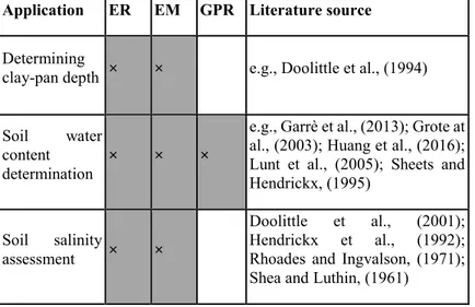
Geophysical methods have been becoming an increasingly valuable tool for application within a variety of agro-ecosystems (Table 2.1).

Geophysical methods, such as electromagnetism, ground penetrating radar, electrical resistivity, do not affect the soil structure and the resulting measurement overlays a first level of spatial variability at different scales.

Table 2.1 Potential agricultural applications for resistivity

(ER), electromagnetic induction (EM), and ground-penetrating radar methods (GPR) (modified from Allred et al., 2008)

Application ER EM GPR Literature source

Determining

clay-pan depth × × e.g., Doolittle et al., (1994)

Soil water content

determination × × ×

e.g., Garrè et al., (2013); Grote at al., (2003); Huang et al., (2016); Lunt et al., (2005); Sheets and Hendrickx, (1995)

Soil salinity

assessment × ×

Doolittle et al., (2001); Hendrickx et al., (1992); Rhoades and Ingvalson, (1971); Shea and Luthin, (1961)

(39)

17

For an agriculture prospective, geophysical applications have been explored mainly in relation to soil moisture and salinity detection, as well as the structural status of surface soil layers (Samouëlian et al., 2005).

Agricultural geophysics measurements can be applied at a wide range of scales and often exhibit significant variability both temporally and spatially (Allred et al., 2008). Agricultural geophysics investigations are commonly (although certainly not always) focused on delineating small- and/or large-scale objects/features within the soil profile also over very large areas.

Agricultural geophysics tends to be heavily focused on a two meters zone directly beneath the ground surface, which includes the crop root zone and all, or at least most, of the soil profile. With regard to the application of geophysics to agriculture, this extremely shallow depth of interest is certainly an advantage, in one sense because most geophysical methods have investigation depth capabilities that far exceed two meters (Allred et al., 2008). The ability to image and quantify soil-moisture changes at important spatial and temporal scales with minimal disturbance to the environment and the possibility to acquire data in difficult terrain are two additional advantages.

The development of geophysical methods (Allred et al., 2008; Vereecken et al., 2006; Binley et al., 2015) provides potentially effective approaches to the challenges above (e.g. Bitella et al., 2015), especially when the study of soil–root plant interactions plays a fundamental role. In particular, the specificity of plant root distribution dynamics (e.g., due to

(40)

18

growth, phenological stage, water and nitrogen availability) and soil texture variability, combined with the pulsed nature of water inputs, create highly heterogeneous situations, in terms of root water uptake (RWU) patterns. These patterns can be difficult to capture even with dense networks of point sensors (Jayawickreme et al., 2014) (e.g., dielectric based). In this respect, there is a growing demand of near-surface observing technologies for studying a wide spectrum of phenomena in the soil, which may have implications also in the agricultural context (Bitella et al., 2015).

Recent studies (Cassiani et al., 2015; Consoli et al., 2016 b; Satriani et al., 2015) have demonstrated that geophysical techniques can support the irrigation operations in terms of both water amounts and irrigation timing. In this context, geophysical imaging techniques are being recognised as very attractive tools for the identification of water dynamics in the vadose zones (e.g. Binley et al., 2002; Deiana et al., 2007, 2008; Cassiani et al., 2012, 2015, 2016).

2.1.1. Electrical resistivity tomography

Electrical resistivity tomography (ERT – see Binley and Kemna, 2005) is an active source geophysical method that uses a low-frequency electrical current, galvanically injected into the ground between two electrodes (current source electrodes), and measures the potential between two or more different electrodes (potential electrodes). This pattern is repeated through many combinations of transmitting and receiving electrodes along a line or grid (or with borehole electrodes), and the result is a cross section or a volume distribution of electrically resistive or conductive regions in

(41)

19

the subsurface. The current, voltage, electrode spacing, and electrode configuration are used to calculate the apparent resistivity (i.e., the inverse of electrical conductivity). As reported above, ERT in general is a technique suitable for the investigation of ground properties, based on the response of soil materials to the flux of electrical charges.

ERT prospecting has recently improved with respect to measurement time. The improvement of computer-controlled multi-channel resistivity-meters using multi-electrode arrays has led to an important development of electrical imaging. Switching units allow any combination of four electrodes to be connected to the resistivity-meter at any time. The electrical data measurement is then fully automated and acquisition can be rapid (Binley et al., 1996).

2.1.1.1 Measurement errors

Assess the data quality is the first step in the direct current (DC) resistivity data processing.

Binley et al (2015b) underline that DC resistivity data can suffer from a range of sources of error, which, if not addressed correctly can have a significant impact on the interpretation of survey results. Binley et al (2015b) report useful recommendation to control measurement errors. Firstly, high contact resistance between the measurement electrodes and the ground can be particularly problematic especially in dry soil. Secondly, it is important to take into account the receiver voltage levels in a given measurement: high geometric factors, combined with low input voltage can

(42)

20

lead to voltages that are close to instrument resolution. Thirdly, natural self-potentials also need to be accounted for particularly if they are not stable over time.

Finally, negative apparent resistivity values in DC resistivity surveys often highlight problems with contact resistance and signal strength. Such measurements may be assessed to be erroneous, however, through appropriate modeling, these measurements provide information about the subsurface and should not be rejected on the grounds of polarity alone. The quality of DC resistivity measurements is often determined through repeatability, i.e. by assessing the variability of responses from multiple injected cycles. Whilst these are useful direct in-field indicators of data quality, sources of error may not be random and could, in theory, repeat. An alternative measure of data quality is reciprocity (e.g. Parasnis, 1988). Measurements made after switching injection and receiver pairs should be identical; the difference is often termed a reciprocal error and can often be a much better assessment of data quality in DC resistivity surveys (see, Slater and Binley, 2006).

2.1.1.2 Modelling and inversion

Whereas the forward model (Fm) computes the apparent

resistivity from a spatial distribution of resistivity, the inverse model derives the set of spatial geoelectrical properties that is consistent with the observed data (apparent resistivity) (Binley et al., 2015b).

(43)

21

The goal is to derive the distribution of the electrical properties (resistivity model) that satisfy the transfer resistance observations for a given set of measurements (resistance data, i.e., the ratio between potential and current), within a specified tolerance level and appropriate model constraints.

Unconstrained inverse modelling of geoelectrical data is inherently non-unique (often underdetermined, too many unknowns and too few equations), in that there are likely to exist a large number of geoelectrical models (e.g. distributions of resistivity) that comply with the observed data. The solution varies, depending on how the problem is posed. Furthermore, without appropriate constraints, errors (e.g. numerical rounding errors) can propagate and lead to an unstable solution.

As reported in Binley et al., (2015b) most geoelectrical inverse models used today are based on a least squares fit between data and model parameters. The data-model misfit is expressed as:

(2.1) where d is the objective function; d are the data (e.g.

measured apparent resistivities); F(m) is the set of equivalent forward model estimates with parameter set m; Wd is a data

weight matrix, which, if we consider the uncorrelated measurement error case and ignore forward model errors, is a diagonal matrix with entries equal to the standard deviation



d F(m)



WTW_d



d F(m)



d

T

d   

(44)

22

of each measurement, quantified using the reciprocal error (Slater et al., 2000).

Attempts have been made to minimize d in Eq. (2.1). Binley

et al., (2015b) report that the Occam’s method proposed by Constable et al.(1987) offered a major breakthrough in geoelectrical inverse modelling and is fundamental to the majority of inverse solutions of DC resistivity today. The method of Constable et al. (1987) searches for the smoothest model (set of parameters) that is consistent with the data. The label “Occam’s” was used by Constable et al. (1987) to emphasize the search for the simplest model (after Occam’s razor). Their approach utilizes spatial regularization (Tikhonov and Arsenin, 1977) to enforce smoothing, which also helps ensure a stable and unique solution. Regularizing the minimization problem can be achieved by adding a model penalty term:

(2.2) where R is a roughness matrix that describes a spatial connectedness of the parameter call values. Then, the function to be minimized is:

(2.3) where  is is a regularization parameter which optimizes the trade-off between the minimized data misfit and the minimized model (i.e., controls the emphasis of smoothing). In an Occam’s solution we seek to satisfy the minimization of equation 2.3, subject to the largest value of α. The process

Rm mT m   m d tot     

(45)

23

is achieved by utilizing the Gauss Newton approach, which results in the iterative solution of:

(2.4)

where J is the Jacobian (or sensitivity) matrix, given by

Ji,j=di/mi; mk is the parameter set at iteration k; m is the

parameter update at iteration. For the DC resistivity case, the inverse problem is typically parameterized using log-transformed resistivity.

The conventional regularization approach in ERT provides an additional constraint to make the problem less underdetermined by favouring models with minimum structure over rougher models that might fit the data equally well (de Groot-Hedlin and Constable, 1990).

2.1.1.3 Time-lapse inversion

Individual images corresponding to different times can be combined and inverted as ratio or differences. If we have two datasets, dt and d0 then we can compute a combined (ratio)

dataset from:

(2.5) where dr is the resistance ratio, dt e d0 are the dataset collected

at the time (t) and at the initial condition (0), and F(ohm) is

resistance value obtained by running the forward model for an arbitrarily chosen conductivity (100 Ohm m). The inverted



_k



_k T d T d T d T_W _J _R _m _J _W _d _F _m _Rm J   )   ( )  ( m m m_k_1  _k  ) ( _hom 0  F d d d t r 

(46)

24

image will then show any changes relative to this reference value.

2.1.2. ERT: application in agricultural contexts

Among the geophysical applications in agriculture and more generally for environmental purposes, electrical resistivity tomography (ERT) is considered one of the most effective methods, as it offers high spatial (and temporal) resolution, combined with a non-invasive character causing no disturbance during soil monitoring (Michot et al. 2003; al Hagrey 2007).

ERT is a minimally invasive technique that obtains information on the variability of the electrical resistivity of the subsoil which, when related to water and solute content, can help to spatialize water and nutrient uptake active zones (e.g. Srayeddin and Doussan, 2009).

Several authors have successfully used ERT to observe transient state phenomena in the soil-plant (SP) continuum. In particular, ERT and other electrical techniques have been adopted to monitor RWU processes of herbaceous crops both in the laboratory (Werban et al., 2008) and at field scale (e.g., Srayeddin and Doussan, 2009; Garré et al., 2011; Beff et al., 2013; Cassiani et al., 2015; Shanahan et al., 2015; Consoli et al., 2016 a and b). These results have demonstrated the match between the temporal soil water content (SWC; m3_m-3₎

changes and the electrical resistivity patterns.

Using the 2-D time-lapse ERT monitoring, Michot et al. (2003) identified the soil drying patterns in the shallow soil

(47)

25

where roots activity is more intense. Other authors applied ERT to eco-physiological studies involving fruit crops such as orange (Cassiani et al., 2015; Moreno et al., 2015), apple (Boaga et al., 2013), olive and poplar trees (al Hagrey, 2007) as well as natural forest (Nijland et al., 2010; Robinson et al., 2012).

Brillante et al. (2015), however, noted that the use of ERT in eco-physiological studies, coupled with parallel monitoring of plant water status, is still rare and therefore needs further investigation in order to answer to new questions on plant and soil relationships, and open the way to new techniques for water management in agricultural scenarios.

The studies highlighted above, show the potential of ERT for these applications, even if difficulties in the interpretation of the measured electrical resistivity patterns remain a frequent limitation especially under field conditions. First, electrical resistivity is a function of a number of soil properties, including the nature of the solid constituents (particle size distribution, mineralogy), the arrangement of voids (porosity, pore size distribution, connectivity), the degree of water saturation (water content), the pore electrical conductivity (solute concentration) and temperature. The variability of these factors needs to be restricted (e.g., adopting time-lapse measurements) or measured independently and a fitting calibration equation needs to be established (e.g., Michot et al., 2003). Second, rapid changes in the soil-plant-atmosphere

continuum, such as an infiltration front passing after

irrigation inputs and/or a heavy rain, require high temporal resolution of the measurement to avoid temporal aliasing (e.g., Koestel et al., 2009). Finally, RWU processes are highly

(48)

26

spatially variable and require at least a decimetric spatial resolution (Michot et al., 2003).

2.2. Overview of evapotranspiration and sap-flow fluxes measurements

2.2.1 Micro-meteorological methods

Evapotranspiration (ET) is the term used to describe the part of the water cycle which removes liquid water from an area with vegetation and into the atmosphere by the processes of both transpiration and evaporation (Allen et al., 1998). From an energetic point of view, Rana and Katerji (2000) described ET as the energy employed for transporting water from the leaves and plant organs to the atmosphere as vapour. The amount of energy, that is at the base of the ET process, is the latent heat (λE, with λ latent heat of vaporization equal to 2.45x106_{J kg}-1_{at 20 °C) and is expressed as energy flux}

density (W m-2_).

Under this form, ET can be measured with the so-called micrometeorological methods. These techniques are physically-based and depend on the laws of thermodynamics and on the transport of scalars into the atmosphere above the canopy. Katerji and Rana (2008) report that micrometeorological applications need accurate measurements of meteorological variables on a short temporal scale with suitable sensors placed above the canopy. Due to the conservative hypothesis of all the flux densities above the crop, the micrometeorological methods can be

(49)

27

applied only on large flat surfaces with uniform vegetation. Micrometeorological methods for measuring or estimating ET are generally referred to plot scale.

2.2.1.1. Eddy covariance technique

The transport of scalar (vapour, heat, carbon dioxide) and vectorial quantities (i.e., momentum) in the low atmosphere in contact with the canopies is mainly driven by air turbulence (Rana and Katerji, 2000; Katerji and Rana , 2008).

The eddy covariance (EC) method is a direct measurement of a turbulent flux density of a scalar across horizontal wind streamlines (Paw U et al., 2000).The calculation of turbulent fluxes is based on the Navier-Stokes equation and similar equations for temperature or gases by the use of the Reynolds' postulates. For details on the theory, see Stull (1988). The equations for determination of surface fluxes are obtained by further simplifications, these are:

 stationarity of the measuring process;

 horizontal homogeneity of the measuring field;  validity of the mass conservation equation;  negligible density flux;

 statistical assumptions, for example statistical independence and the definition of the averaging procedure;

 the Reynolds' postulates and the postulate which is used for the calculation of the eddy covariance method should be valid;

(50)

28

 the momentum flux in the surface layer as well as the temperature flux (analogue equations for water vapour and gaseous fluxes) doesn't change with the height within about 10% to 20% of the flux (Foken and Wichura, 1996).

When certain assumptions are valid, theory predicts that energy fluxes from the surface can be measured correlating to the vertical wind fluctuations from the mean (w’) in concentration of the transported admixture (Rana and Katerji, 2000). A direct method for measuring λE, above a vegetative surface over a homogeneous canopy, is to measure simultaneously vertical turbulent velocity and specific humidity fluctuations and to determine their covariance over a suitable sampling time. So that, for latent heat flux (E) we can write the following covariance of vertical wind speed and vapour density: ' ' q w E    (2.6)

with w’ is the vertical wind speed (m s-1_{) and q’ is the air}

humidity (kg m-3_).

In this way, measurements of the instantaneous fluctuations of w’ and q’, at a frequency sufficient for obtaining the contribution from all the significant sizes of eddy, permit to calculate ET by summing their product over a hourly time scale. To measure ET with this method, vertical wind fluctuations must be measured and acquired at the same time as the vapour density. The first one can be measured by a

(51)

29

sonic anemometer, the second one by a fast response hygrometer (Katerji and Rana, 2008).

The sensible heat (H) using the EC technique by analogy with the expression above (Eq. 2.6), can be written as

' 'T w c

H _air _p (2.7)

with airthe air density and cp the specific heat of air at a

constant pressure.

The wind speed (w’) and temperature fluctuations (T’) are measured by means of sonic anemometer and fast response thermometer, respectively (Katerji and Rana, 2008).

Sensors must measure vertical velocity, temperature and humidity with sufficient frequency response to record the most rapid fluctuations important to the diffusion process. Typically, a frequency of the order of 5-10 Hz is used, but the response-time requirement depends on wind speed, atmospheric stability and the height of the instrumentation above the surface. Outputs are sampled at a sufficient rate to obtain a statistically stable value for the covariance (Drexler et al., 2004). If a 30-minute sampling time is used over the whole day, then remarkable errors will be reduced (Foken, 2008). Wind speed and humidity sensors should be installed close to each other but sufficiently separated to avoid interference. When the separation is too large, underestimation of the flux may result. Some disadvantages of EC method include sensitivity to fetch and high cost and maintenance requirements (Brotzge and Crawford, 2003;

(52)

30

Foken, 2008). High-frequency wind vector data are usually obtained with a three-dimensional sonic anemometer. These instruments provide the velocity vector in all three directions and, therefore, corrections can be applied for any tilt in the sensor and mean streamline flow. A wide range of humidity sensors have been used in EC systems including thermocouple psychrometers, Lyman-alpha and krypton hygrometers, laser-based systems and other infrared gas analysers (Drexler et al., 2004). Since the size of the turbulence eddies increases with distance above the ground surface, both the measuring path length and the separation between a sonic anemometer and an additional device depend on the height of measurement. Therefore, to reduce the corrections of the whole system the measurement height must be estimated on the basis of both the path length of the sonic anemometer and the separation of the measuring devices. In addition, the measuring height should be twice the canopy height in order to exclude effects of the roughness sublayer (Foken, 2008).

The EC technique is the most direct method for quantifying the turbulent exchange of energy and trace gases between the Earth’s surface and the atmosphere (Mauder et al., 2010). However, the derivation of the mathematical algorithm is based on a number of simplifications so that the method can be applied only if these assumptions are exactly fulfilled. The quality of the measurements depends mainly on the application conditions and accurate use of the corrections than on the available highly sophisticated measuring systems. Therefore, experimental experience and knowledge of the special atmospheric turbulence characteristics have a high

(53)

31

relevance. The most limiting conditions are horizontally homogeneous surfaces and steady-state conditions (Foken, 2008a). These requirements are often violated in complex terrain, and their non-fulfilment reduces the quality of the measurement results. Foken and Wichura (1996) address this problem by assigning quality flags to the fluxes in accordance with the deviations found between parameterisations under ideal conditions and those actually measured. Secondly, in a heterogeneous environment the land use types contributing to the measurements change with the source area of the fluxes. This source area, which can be calculated by footprint models, defines the region upwind of the measurement point, which influences the sensor’s measurements and is dependent on measurement height, terrain roughness, and boundary layer characteristics, such as the atmospheric stability. As most sites in monitoring networks are set up to measure fluxes over a specific type of vegetation, the changing contribution of this type of land use, under different meteorological conditions, has to be considered in order to assess how representative the measurements are (Göckede et al., 2004). The latter can lead to a bias of the flux estimate that becomes apparent in a lack of energy balance closure, usually ranging between 10 and 30% of the available energy at the surface. It is possible to minimize the deviation between actual and measured EC fluxes through an optimal equipment configuration and through application of adequate correction methods. The typical processing steps are:

 tilt correction,

(54)

32

 density correction (also WPL correction, see Webb et al. 1980),

 damping (attenuation) correction (Spank and Bernhofer, 2008).

The application of correction methods is closely connected with the data control. The data control starts with the exclusion of missing values and outliers. A basic condition for applying the EC method is the assumption of a negligible mean vertical wind component; otherwise, advective fluxes must be corrected. This correction is called tilt correction and includes the rotation of a horizontal axis into the mean wind direction. The first correction is the rotation of the coordinate system around the z-axis into the mean wind. The second rotation is around the new y-axis until the mean vertical wind disappears. With these rotations, the coordinate system of the sonic anemometer is moved into the streamlines (Foken, 2008). An important correction to the actual available turbulence spectra is the adjustment of the spectral resolution of the measuring system. Hence, the resolution in time (time constant), the measuring path length, and the separation between different measuring paths must be corrected. The spectral correction is made using transfer functions (Foken, 2008). WPL-correction is a density correction, caused by ignoring density fluctuations, a finite humidity flux at the surface, and the measurement of gas concentration per volume unit instead of per mass unit. WPL-correction is large if the turbulent fluctuations are small relative to the mean concentration. The conversion from volume into mass-related values using WPL-correction is not applicable if the water vapour concentrations or the concentrations of other gases are

(55)

33

transferred into mol per mol dry air before the calculation of EC. However, the calculation is possible depending on the sensor type and if it is offered by the manufacturers (Foken, 2008). Hence, the quality assurance of turbulence measurements with EC method is a combination of the complete application of all corrections and the exclusion of meteorological influences such as internal boundary layers, gravity waves, and intermitted turbulence. Quality tests are used to validate the theoretical assumptions of the method such as steady-state conditions, homogeneous surfaces, developed turbulence (Foken, 2008).

2.2.2 Sap flow by heat pulse technique

This method measures the water loss at the plant scale. Sap flow is closely linked to plant transpiration (TSF) by means of

simple accurate models (Katerji and Rana, 2008). Sap flow methods are easily automated, so continuous records of plant water use with high time resolution can be obtained. Moreover, these methods can be used anywhere with minimally disturbance at the site. However, when sap flow measurements are adopted to estimate TSF for stands of

vegetation, appropriate methods of scaling from plant to unit area of land must be used (Smith and Allen, 1996).

Different methods are used to measure sap flow in plant stems or trunks. The most common are: heat pulse velocity (HPV) methods; heat balance method; thermal dissipation probe method or Granier method. In HPV methods, sap flow is estimated by measuring HPV, stem area and xylem conductive area (Katerji and Rana, 2008), using a linear heater and temperature probes inserted radially into the plant