Research Article
On the Effect of Labour Productivity on Growth: Endogenous
Fluctuations and Complex Dynamics
F. Grassetti
, C. Mammana
, and E. Michetti
Department of Economics and Law, University of Macerata, Macerata, Italy
Correspondence should be addressed to C. Mammana; [email protected] Received 3 April 2018; Accepted 5 September 2018; Published 9 October 2018 Academic Editor: Josef Dibl´ık
Copyright © 2018 F. Grassetti et al. This is an open access article distributed under the Creative Commons Attribution License, which permits unrestricted use, distribution, and reproduction in any medium, provided the original work is properly cited. This paper introduces a sigmoidal production function that considers production possible even when the only input is labour. The long-run behaviour of an economy described by the neoclassical Solow-type growth model with differential savings is investigated considering the technology presented. It is found that labour productivity influences the existence of boom and bust periods as well as the level of capital per capita in equilibrium.
1. Introduction
Economic growth models explain a country’s capital accumu-lation over time. One of the most used neoclassical models is the model developed by Solow and Swan (see Solow [1] and Swan [2]). The Solow-Swan model considers the growth rate of labour, the depreciation rate of capital, the saving rate, and the technology of production as determinants of the long-run behaviour of an economy. An extension of the Solow model considers two different saving propensities for workers and shareholders (see B¨ohm and Kaas [3]).
In literature, different technologies have been studied in the Solow framework to analyse the evolution of capital per capita over time. Production technologies with Constant Elasticity of Substitution between production factors (see Brianzoni [4, 5], Masanjala and Papageorgiou [6], and Papa-georgiou and Saam [7]) and Variable Elasticity of Substitution (see Brianzoni et al. [8], Cheban et al. [9], and Karagiannis et al. [10]) have been considered in order to verify which parameters influence the generation of cycles and of more complex dynamics for an economy. It has been found that nonsimple dynamics arise when the elasticity of substitution is sufficiently low and shareholders save more than workers. Moreover, attention has been paid to sigmoidal production functions (see Brianzoni et al. [11, 12]), since they are able to describe growth dynamics of nondeveloped and developing countries.
In all the above-mentioned works the technology con-sidered,𝑓(𝑘), satisfies 𝑓(0) = 0, where 𝑘 is the capital per capita. Therefore, all those works provide a production rule for which no capital can be generated without capital. Thus, they do not take into consideration a possibility of deriving from one of the assumptions of the Solow model: in his work, Solow [1] defined the capital stock as the amount of already-produced output. This implies that an initial production of capital should be possible when the only production factor is labour. Moreover, it is known that nondeveloped countries may base their early stage development only on labour (agriculture and handicraft manufacture), as Azariadis and Stachurski [13]) discussed.
In this paper we present a sigmoidal technology that satisfies 𝑓(0) > 0, providing the condition for an initial amount of production possible without capital. We then investigate the Solow-type model with differential savings considering the technology introduced, in order to verify how the long-run behaviour of an economy is influenced by labour productivity (a measure of the quantity of output that can be produced from labour).
The rest of the paper is organised as follows. In Section 2 we describe the production function, in Section 3 we study the existence and stability of the steady states, while in Section 4 we investigate the influence of labour productivity on long-run dynamics. Section 5 concludes the paper.
Volume 2018, Article ID 6831508, 9 pages https://doi.org/10.1155/2018/6831508
0 10 k 0 4 @M (E ) (a) 0 1.6 0 1.6 EN &(E N ) (b)
Figure 1: (a) Production function𝑓𝑠(𝑘𝑡) for 𝛼 = .5, 𝛽 = .2, 𝜌 = 3, and 𝑐 = 1. (b) Map 𝐹(𝑘𝑡) and its fixed points for 𝑛 = 𝑠𝑤 = .2, 𝛿 = 𝑠𝑟= .7, 𝛼 = 1, 𝛽 = .5, and 𝑐 = 𝛼(𝜌 − 1)2/4𝛽𝜌; one fixed point for 𝜌 = 2.5 (green map), two fixed points for 𝜌 = 2.8 (purple map), and three fixed
points for𝜌 = 3.2 (blue map).
2. Model Setup
Nonconcave production functions are used in literature to describe countries with a low level of economic development, since they present increasing returns to scale at an early stage of development and diminishing ones at a later stage (see, among all, Skiba [14] who introduced them). Capasso et al. [15] presented the sigmoidal production function mapping capital per worker into output per worker, as given by
𝑓 (𝑘𝑡) = 𝛼𝑘𝜌𝑡
1 + 𝛽𝑘𝜌𝑡 (1)
where 𝛼 and 𝛽 are nonnegative and 𝜌 ≥ 2 is the output elasticity of capital. Notice that an inflection point𝑘𝑓exists such that𝑓(𝑘𝑡) is convex for 𝑘𝑡 ∈ (0, 𝑘𝑓) and it is concave for 𝑘 ∈ (𝑘𝑓, +∞) with 𝑘𝑓 = ((𝜌 − 1)/𝛽(𝜌 + 1))1/𝜌, so it is a convex-concave production function. Such a function can be considered an extension of the Cobb–Douglas (CD) production function, since it approximates the CD case when 𝛼 = 1 and 𝛽 = 0. Notice that 𝑓(𝑘) does not fulfil the Inada Conditions (see Barro and Sala-i Martin [16]), being lim𝑘→0𝑓(𝑘) = 0. The S-shape behaviour of the function allows us to consider less-developed countries, but it does not take into account those economies driven by craftsmanship, i.e., in which low levels of output are possible even without capital, that is, with𝑓(0) > 0. In order to consider these economies, we add a positive constant 𝑐 to the sigmoidal production function. The resulting shifted sigmoidal (SS) production function is given by
𝑓𝑠(𝑘𝑡) = 𝛼𝑘𝜌𝑡
1 + 𝛽𝑘𝜌𝑡 + 𝑐 (2)
and its graph is in Figure 1(a).
Notice that when the SS production function is consid-ered, production is possible without capital, being 𝑓𝑠(0) = 𝑐 > 0. This kind of technology has been already considered in literature when studying the evolution of capital per capita over time (see, among all, the Nobel Prize Solow [1]).
We now consider the wage of a worker. When the per capita wage of a worker equals the marginal product of labour,
that is, 𝑤(𝑘𝑡) = 𝑓(𝑘𝑡) − 𝑘𝑡𝑓(𝑘𝑡), and the SS production function is considered, then the wage is given by
𝑤 (𝑘𝑡) =𝛼𝑘 𝜌 𝑡(𝛽𝑘𝜌𝑡 − 𝜌 + 1) (𝛽𝑘𝜌𝑡 + 1)2 + 𝑐 (3) being 𝑓𝑠(𝑘𝑡) = 𝛼𝜌𝑘𝜌−1𝑡 (1 + 𝛽𝑘𝜌𝑡)2. (4) In order for the wage to be nonnegative, we assume 𝑐 ≥ (𝛼/𝛽)((𝜌 − 1)2/4𝜌) = 𝑐min, so that the minimum point of 𝑤(𝑘) is either positive or equal to zero. This consideration establishes an economically meaningful lower bound of𝑐 for the setup, as stated in the following remark.
Remark 1. The shifted sigmoidal production function (SS) is given by
𝑓𝑠(𝑘𝑡) = 𝛼𝑘𝜌𝑡
1 + 𝛽𝑘𝜌𝑡 + 𝑐 (5)
where𝛼 ≥ 0, 𝛽 ≥ 0, 𝜌 ≥ 2, and 𝑐 ≥ (𝛼/𝛽)((𝜌 − 1)2/4𝜌) for the wage being nonnegative.
As it can be observed in Figure 1(a), the SS production function describes economies in which output is generated even without capital. Recall that the elasticity of substitution (ES) between production factors measures the ease with which capital and labour can be substituted for one another and, for twice differentiable production functions, it is math-ematically defined by (see Sato and Hoffman [17]):
𝜎 (𝑘) = −𝑓 (𝑘) (𝑓 (𝑘) − 𝑘𝑓(𝑘)) 𝑘𝑓 (𝑘) 𝑓(𝑘) . (6) Being 𝑓𝑠(𝑘𝑡) = −𝛼𝜌𝑘 𝜌−2 𝑡 (𝛽 (𝜌 + 1) 𝑘𝜌𝑡 − 𝜌 + 1) (𝛽𝑘𝜌𝑡+ 1)3 (7) and the SS production function as given by (2), the resulting ES is
𝜎 (𝑘𝑡) = 𝑐 (𝛽𝑘 𝜌
𝑡 + 1)2+ 𝛼𝑘𝜌𝑡(𝛽𝑘𝜌𝑡− 𝜌 + 1)
Therefore, this production function belongs to the class of VES (Variable Elasticity of Substitution) production func-tions, since𝜎 depends on the capital per capita level. Notice that the ES may be negative. Production functions with negative ES between inputs can be found in literature (see, among all, Prywas [18], Thompson and Taylor [19], Jurgen [20], and Grassetti et al. [21]). The work of Paterson [22] suggests that such eventuality occurs when production inputs are complementary.
Consider now the Solow-Swan-type growth model in which workers and shareholders have different but constant saving rates (respectively,𝑠𝑤 ∈ (0, 1) and 𝑠𝑟 ∈ (0, 1)) and assume that shareholders receive the marginal product of capital𝜋(𝑘), while the wage rate 𝑤(𝑘) equals the marginal product of labour. Following B¨ohm and Kaas [3], the map describing the capital accumulation over time𝑡 ∈ N is then given by 𝑘𝑡+1= 𝐹 (𝑘𝑡) = 1 1 + 𝑛[(1 − 𝛿) 𝑘𝑡+ 𝑠𝑤𝑤 (𝑘𝑡) + 𝑠𝑟𝜋 (𝑘𝑡)] , 𝑘𝑡≥ 0 (9)
where the labour force grows at a rate𝑛 ≥ 0 and 𝛿 ∈ (0, 1] is the depreciation rate of capital.
In order to consider less-developed economies, in which production is possible using only labour, we assume that the technology is described by the SS production function as defined in (5). Consequently, the per capita wage of workers is given in (3), while the income per worker of a shareholder is given by
𝜋 (𝑘𝑡) = 𝛼𝜌𝑘𝜌𝑡
(1 + 𝛽𝑘𝜌𝑡)2. (10) Taking into account (9), (3), and (10), the final continuous and smooth one-dimensional map describing the capital per capita evolution is given by
𝑘𝑡+1= 𝐹 (𝑘𝑡) = 1 + 𝑛1 [(1 − 𝛿) 𝑘𝑡+ 𝑠𝑤𝛼𝑘 𝜌 𝑡 1 + 𝛽𝑘𝜌𝑡 +(𝑠𝑟− 𝑠𝑤) 𝛼𝜌𝑘𝜌𝑡 (1 + 𝛽𝑘𝜌𝑡)2 + 𝑠𝑤𝑐] , (11)
where𝐹(𝑘𝑡) ≥ 0 ∀𝑘𝑡 ≥ 0 for all combinations of parameter values. Notice that in Brianzoni et al. [11], where a sigmoidal production function is considered, the condition𝑠𝑟 ≥ 𝑠𝑤is required in order to assure that𝐹(𝑘𝑡) is nonnegative for all 𝑘𝑡. Differently, if the SS production function (as defined in Remark 1) is considered, then the final map𝐹(𝑘𝑡) has always economic meaning, thus allowing us to consider both cases 𝑠𝑟 ≥ 𝑠𝑤and𝑠𝑟 < 𝑠𝑤and, therefore, this can be considered a generalisation of the previous work. This is possible because capital is not an essential input for production and hence even an economy where shareholders are not saving can be considered.
3. Equilibria and Local Dynamics
In this section we consider the question of the existence and stability of steady states for an economy described by the Solow-Swan growth model with differential savings as proposed in B¨ohm and Kaas [3], while considering the SS production function as defined in Remark 1.
3.1. Existence of Steady States. We now analyse the number of steady states map 𝐹 may own, considering different conditions on parameters values.
The first difference from most of the models that consider the same initial framework (see, among all, Brianzoni et al. [12] and Klump and de La Grandville [23]) concerns the existence of a steady state characterised by zero capital per capita. While previous works established the existence of this equilibrium, when the SS production function is considered, the origin is not a fixed point, being𝐹(0) > 0. This happens when production is possible without capital (i.e., only labour is necessary), as the works of Solow [1] and Miyagiwa and Papageorgiou [24] demonstrate. Notice that this model better describes the behaviour of nondeveloped economies: even in those countries in which only labour is available (no infrastructures, machineries, or investments are given), a minimum level of production is possible, i.e., agriculture and handicraft manufacture (with regard to the early stages of economic development see Azariadis and Stachurski [13]). While Brianzoni et al. [11] proved that, when the sigmoidal production function given by (5) is considered, a poverty trap exists (the origin is a stable fixed point); this work found that, if a technology in which the only necessary input factor is labour is considered, the existence of the ’vicious circle of poverty’ (see Azariadis and Stachurski [13]) can be avoided. Notice that, even though an economy in which only labour is given will not converge to a zero growth rate, attention should be paid to the existence of multiple positive steady states: different equilibrium levels of capital per capita would explain the coexistence of nondeveloped, developing, and developed countries.
To this aim we now consider the following functions: 𝐺 (𝑘𝑡) = 𝑘𝜌−1𝑡 1 + 𝛽𝑘𝜌𝑡 (𝑠𝑤+ 𝜌 Δ𝑠 1 + 𝛽𝑘𝜌𝑡) (12) and 𝐻(𝑘𝑡) =𝑛 + 𝛿𝛼 −𝑠𝑤𝑐 𝛼𝑘𝑡, (13)
withΔ𝑠= 𝑠𝑟− 𝑠𝑤∈ (−𝑠𝑤, 1 − 𝑠𝑤). Then the fixed points of (11) are the solutions of equation𝐺(𝑘𝑡) = 𝐻 (𝑘𝑡), 𝑘𝑡≥ 0.
As far as the properties of function𝐺(𝑘𝑡) are concerned, the following proposition holds.
Proposition 2. Function 𝐺(𝑘𝑡) as given by (12) is defined ∀𝑘𝑡 ≥ 0, it is continuous and differentiable such that 𝐺(0) = lim𝑘𝑡→+∞𝐺(𝑘𝑡) = 0. Furthermore, there exist 0 < 𝑘𝑚 < 𝑘𝑀 such that
(i) if((𝜌 − 1)/𝜌)𝑠𝑤 ≤ 𝑠𝑟 < 1, then 𝐺(𝑘𝑡) admits a unique maximum point𝑘𝑀;
(ii) if0 < 𝑠𝑟< ((𝜌−1)/𝜌)𝑠𝑤, then𝐺(𝑘𝑡) admits a minimum point𝑘𝑚and a maximum point𝑘𝑀,0 < 𝑘𝑚 < 𝑘𝑀. Proof. The first part is trivial. As far as the number of critical points of𝐺(𝑘𝑡) is concerned, it is possible to write
𝐺(𝑘𝑡) = 𝑓 (𝑘𝑡) 𝛼 (1 + 𝑀)2𝑘2 𝑡 (𝑎1 𝑀2+ 𝑎2𝑀 + 𝑎3) (14) where𝑓(𝑘𝑡) is given by (1), 𝑀 = 𝛽𝑘𝜌𝑡,𝑎1 = −𝑠𝑤,𝑎2 = 𝑠𝑤(𝜌 − 2) − (𝜌2+ 𝜌)Δ 𝑠, and𝑎3= 𝑠𝑤(𝜌 − 1) + (𝜌2+ 𝜌)Δ𝑠.
(i) Consider Δ𝑠 > 0, then 𝐺(𝑘𝑡) admits a unique maximum point given by𝑘𝑀= [(−𝑎2−√𝑎22− 4𝑎1𝑎3)/ (2𝑎1𝛽)]1/𝜌as it was proved in Brianzoni et al. [11]. (ii) ConsiderΔ𝑠< 0, then 𝑎1 < 0, 𝑎2 > 0 while 𝑎3can be
positive or negative. Define𝑍(𝑀) = 𝑎1𝑀2+ 𝑎2𝑀 + 𝑎3 and notice that𝑍(0) > 0. Then
(a) if𝑎3 ≥ 0, i.e., 𝑠𝑟 ≥ ((𝜌 − 1)/𝜌)𝑠𝑤, the equation 𝑍(𝑀) = 0 admits a unique positive solution; hence𝐺(𝑘𝑡) admits a unique maximum point 𝑘𝑀;
(b) if 𝑎3 < 0, 𝑍(𝑀) = 0 may admit two, one, or zero solutions, depending on the sign of 𝑍(−𝑎2/2𝑎1) = −(𝑎2
2 − 4𝑎1𝑎3)/4𝑎1. Notice that 𝑍(−𝑎2/2𝑎1) > 0 iff 𝑎2
2 > 4𝑎1𝑎3. After some computations, it can be observed that this inequality is always verified; hence, if 𝑠𝑟 < ((𝜌 − 1)/𝜌)𝑠𝑤, then 𝑍(𝑀) = 0 admits two solutions. The minimum and maximum points are given, respectively, by 𝑘𝑚 = [(−𝑎2 + √𝑎2
2− 4𝑎1𝑎3)/(2𝑎1𝛽)]1/𝜌 and 𝑘𝑀, where 0 < 𝑘𝑚< 𝑘𝑀.
Taking into account Proposition 2 and considering that 𝐻(𝑘𝑡) given by (13) is a hyperbola with 𝐻(𝑘𝑡) < (𝑛 + 𝛿)/𝛼 ∀𝑘𝑡 > 0, lim𝑘𝑡→0+𝐻(𝑘𝑡) = −∞, lim𝑘
𝑡→+∞𝐻(𝑘𝑡) =
(𝑛+𝛿)/𝛼 > 0, 𝐻> 0, and 𝐻< 0 ∀𝑘
𝑡> 0, then the following proposition holds.
Proposition 3. Map 𝐹(𝑘𝑡) given by (11) admits at least one positive fixed point and at most three positive fixed points.
Proof. Recall that𝐻(𝑘𝑡) is concave, lim𝑘𝑡→+∞𝐻(𝑘𝑡) = (𝑛 + 𝛿)/𝛼 and lim𝑘𝑡→+∞𝐺(𝑘𝑡) = 0.
(i) Assume0 < 𝑠𝑟< ((𝜌−1)/𝜌)𝑠𝑤. Then𝐺(𝑘𝑡) is bimodal with𝑘𝑚 < 𝑘𝑀. Then
(a) if 𝐺(𝑘𝑚) > 𝐻 (𝑘𝑚) no intersection exists in (0, 𝑘𝑚). Moreover, if 𝐺(𝑘𝑀) ≥ 𝐻 (𝑘𝑀), one intersection exists in[𝑘𝑀, +∞) and at most two intersections may exist in[𝑘𝑚, 𝑘𝑀), whereas if 𝐺(𝑘𝑀) < 𝐻 (𝑘𝑀), no intersection exists in [𝑘𝑀, +∞) and from one up to three intersec-tions exist in(𝑘𝑚, 𝑘𝑀);
(b) if 𝐺(𝑘𝑚) ≤ 𝐻 (𝑘𝑚), one intersection exists in (0, 𝑘𝑚]. Moreover, if 𝐺(𝑘𝑀) ≥ 𝐻 (𝑘𝑀), one inter-section exists in(𝑘𝑚, 𝑘𝑀) and one in [𝑘𝑀, +∞), whereas if𝐺(𝑘𝑀) < 𝐻 (𝑘𝑀), at most two inter-sections exist in(𝑘𝑚, 𝑘𝑀) and no intersection exists in[𝑘𝑀, +∞).
(ii) Assume ((𝜌 − 1)/𝜌)𝑠𝑤 ≤ 𝑠𝑟 < 1. Then 𝐺(𝑘𝑡) is unimodal with maximum point𝑘𝑀. Then
(a) if𝐺(𝑘𝑀) < 𝐻 (𝑘𝑀), from one up to three inter-sections exist in (0, 𝑘𝑀) and no intersection exists in[𝑘𝑀, +∞);
(b) if𝐺(𝑘𝑀) ≥ 𝐻 (𝑘𝑀), one intersection exists in [𝑘𝑀, +∞). Moreover at most two intersections exist in(0, 𝑘𝑀).
Notice that points 𝐺(𝑘𝑀) and 𝐻(𝑘𝑀) determine the position of the higher equilibrium: whatever the saving propensity of shareholders, when𝐺(𝑘𝑀) > 𝐻 (𝑘𝑀), one fixed point exists in the interval[𝑘𝑚, +∞), while no fixed points exist in that interval otherwise.
Differently from previous models using this initial frame-work, when production is possible even without capital, the origin is not a fixed point. Moreover, up to three fixed points may exist (see Figure 1(b)). Notice that the number of fixed points is in agreement with that obtained by Brianzoni et al. [8] and Grassetti et al. [21] considering different types of VES production functions, but, whereas in previous works the condition 𝑠𝑟 ≥ 𝑠𝑤 was required, in this case multiple equilibria may exist even if workers save more than shareholders.
3.2. Local Dynamics. Function𝐹(𝑘𝑡) as given by (11) can be written in terms of function𝐺(𝑘𝑡) as follows:
𝐹 (𝑘𝑡) = 1 1 + 𝑛[(1 − 𝛿) 𝑘𝑡+ 𝛼𝑘𝑡𝐺 (𝑘𝑡)] + 𝑠𝑤𝑐 1 + 𝑛 (15) Hence 𝐹(𝑘𝑡) = 1 + 𝑛1 {1 − 𝛿 + 𝛼𝑆 (𝑘𝑡)} , (16) where 𝑆 (𝑘𝑡) = 𝐺 (𝑘𝑡) + 𝑘𝑡𝐺(𝑘𝑡) = 𝜌𝑘𝜌−1𝑡 [(𝑠𝑤− 𝜌Δ𝑠) 𝛽𝑘𝜌𝑡+ 𝜌Δ𝑠+ 𝑠𝑤] (1 + 𝛽𝑘𝜌𝑡)3 . (17)
Notice that𝐺(0) = lim𝑘𝑡→0+𝑘𝑡𝐺(𝑘𝑡) = 0; hence 𝐹(0) ∈
(0, 1), that is, ∃𝐼+ = (0, 𝑟1) s.t. 𝐹(𝑘𝑡) is strictly increasing ∀𝑘𝑡∈ (0, 𝑟1). Since lim𝑘𝑡→+∞𝐹(𝑘
𝑡) = (1 − 𝛿)/(1 + 𝑛) ∈ (0, 1), then∃𝐼∞ = (𝑟2, +∞) s.t. 𝐹(𝑘𝑡) is strictly increasing ∀𝑘𝑡 ∈ (𝑟2, +∞). Hence, taking into account also the properties of function 𝐺(𝑘𝑡), two cases may occur: 𝐹(𝑘𝑡) is strictly increasing or𝐹(𝑘𝑡) is bimodal; i.e., it admits a minimum point 𝑘minand a maximum point𝑘max. The following proposition holds.
Proposition 4. Consider 𝐹(𝑘𝑡) as given by (11). If 𝑠𝑟 ∈ [((𝜌 − 1)/𝜌)𝑠𝑤, ((𝜌 + 1)/𝜌)𝑠𝑤), then 𝐹(𝑘𝑡) is strictly increasing. Proof. If𝑠𝑤−𝜌Δ𝑠> 0 and 𝑠𝑤+𝜌Δ𝑠≥ 0, then 𝐹(𝑘𝑡) > 0 ∀𝑘𝑡> 0.
Proposition 4 establishes a sufficient condition for the strict monotonicity of𝐹(𝑘𝑡): if this condition is not fulfilled, map 𝐹 can be strictly increasing or bimodal. Notice that, when the condition of Proposition 4 holds and only one equilibrium exists, the long-run behaviour of an economy can be easily understood, as the following proposition states.
Proposition 5. Assume 𝑠𝑟∈ [((𝜌−1)/𝜌)𝑠𝑤, ((𝜌+1)/𝜌)𝑠𝑤), and let𝑘∗be the unique fixed point of map𝐹. Then 𝑘∗is globally stable.
Proof. From Proposition 4 it is known that, when𝑠𝑟∈ [((𝜌 − 1)/𝜌)𝑠𝑤, ((𝜌 + 1)/𝜌)𝑠𝑤), 𝐹(𝑘𝑡) > 0 ∀𝑘𝑡> 0. Moreover, 𝐹(0) > 0 and lim𝑘𝑡→+∞𝐹(𝑘𝑡)−𝑘𝑡< 0. Being 𝑘
∗the only fixed point of 𝐹, i.e., 𝐹(𝑘∗) = 𝑘∗, then𝐹(𝑘𝑡) > (<)𝑘∗ ∀0 ≥ 𝑘𝑡< 𝑘∗(𝑘𝑡> 𝑘∗) and hence𝑘∗is globally stable.
Recall from Proposition 3 that map𝐹 may have from one up to three fixed points. When the condition of Proposition 4 holds and𝐹 has one fixed point, then it is globally stable. Mod-ifying the parameter values, a fold bifurcation occurs (when parameters reach the bifurcation values, one nonhyperbolic fixed point is created) and a pair of fixed points emerges so map𝐹 has three fixed points 𝑘1 < 𝑘2 < 𝑘3(see Figure 1(b)). Being𝐹(𝑘𝑡) increasing, the fixed points are alternatively stable and unstable, with the unstable equilibrium𝑘2that separates the basins of attraction of𝑘1and𝑘3. Notice that, when 3 fixed points exist the model simultaneously explains the behaviour of economies that, starting from different initial conditions, reach different equilibria level of capita per capita in the long-run.
We now focus on the role of labour productivity on growth. Notice that the productivity of labour is the measure of the amount of output produced with one hour’s labour. Moreover, the existence of a positive relation between labour productivity and wage has been demonstrated (see Meager and Speckesser [25]). For the SS production function it has 𝐹(0) = 𝑐; therefore parameter 𝑐 influences the production without capital: when the only input of production is labour, the higher the value of𝑐, the higher the value of output for the economy. Moreover, considering the wage equation as given by (3), it follows that𝜕𝑤(𝑘𝑡)/𝜕𝑐 > 0, so a positive correlation between𝑐 and 𝑤(𝑘𝑡) is evident. Given these considerations, 𝑐 can be seen as an indirect measure of labour productivity. The following proposition highlights the role played by parameter 𝑐 on the existence and position of the equilibrium level of an economy.
Proposition 6. Consider two economies described by SS
tech-nology and differing only in the constant 𝑐, both with only one equilibrium level for capital per capita. Then the one with higher production without capital (i.e., higher value of𝑐) will experience a higher level of capital per capita in the steady states.
Figure 2: Labour productivity, annual growth rate (%),2000−2016. Source: OECD.
Proof. As the proof of Proposition 3 showed, the locations of the steady states depend on the intersection between 𝐺(𝑘𝑡) and𝐻(𝑘𝑡). Recall that 𝐺(𝑘𝑡) has a maximum point 𝑘𝑀and can have a minimum point𝑘𝑚< 𝑘𝑀. Moreover, lim𝑘
𝑡→0+𝐺(𝑘𝑡) =
lim𝑘
𝑡→+∞𝐺(𝑘𝑡) = 0 while 𝐻(𝑘𝑡) is strictly increasing with
lim𝑘
𝑡→0+𝐻(𝑘𝑡) = −∞ and lim𝑘𝑡→+∞𝐻(𝑘𝑡) = (𝑛 + 𝛿)/𝛼.
Notice that parameter𝑐 has no effect on the shape of function 𝐺(𝑘𝑡), while 𝜕𝐻(𝑘𝑡)/𝜕𝑐 < 0, so that 𝐻(𝑘𝑡) shifts downward as 𝑐 increases. Therefore, when only one intersection between 𝐺 and𝐻 exists, a higher value of 𝑐 determines a higher value of the intersection point.
The previous proposition demonstrates a positive cor-relation between labour productivity and the value of the capital stock for the higher steady state. This result is in agreement with the Organisation for Economic Cooperation and Development (OECD) data: as it can be seen in Figure 2, the years of economic crisis are related to lower levels of labour productivity.
Notice that the condition of Proposition 4 is fulfilled when𝑠𝑟 ∈ 𝐼(𝑠𝑤, 𝜖). Therefore, when the saving behaviours of the two income groups are similar, the economy does not experience boom and bust periods (since 𝐹 is strictly increasing, no fluctuation can be generated). To investi-gate the appearance of fluctuations, we now prove that function 𝐹 may be unimodal, depending on parameter values.
Proposition 7. Consider 𝐹 and 𝑆 as given, respectively, by
(11) and (17). Define𝑟 = 𝜌√[(3𝜌2+ 1)Δ𝑠+ 4𝑠𝑤]Δ𝑠+ 𝑠2𝑤and assume𝑘𝑆1 = [(2𝜌2Δ𝑠+ 𝑠𝑤+ 𝑟)/𝛽(𝜌 + 1)(𝜌Δ𝑠− 𝑠𝑤)]1/𝜌and 𝑘𝑆2= [(2𝜌2Δ
𝑠+ 𝑠𝑤− 𝑟)/𝛽(𝜌 + 1)(𝜌Δ𝑠− 𝑠𝑤)]1/𝜌.
Map𝐹 is bimodal with 𝑘max < 𝑘minif one of the following conditions holds:
(i)𝑠𝑟 ≥ ((𝜌 + 1)/𝜌)𝑠𝑤∧ 𝑆(𝑘𝑆2) < (𝛿 − 1)/𝛼; (ii)𝑠𝑟 < ((𝜌 − 1)/𝜌)𝑠𝑤∧ 𝑆(𝑘𝑆1) < (𝛿 − 1)/𝛼. Map𝐹 is strictly increasing otherwise.
Proof. Recall (16). The critical points of 𝐹 are solutions of 𝑆(𝑘𝑡) = (𝛿 − 1)/𝛼. Notice that 𝑆(0) = lim𝑘𝑡→+∞𝑆(𝑘𝑡) = 0. Moreover,𝑆(𝑘𝑡) = 𝜌𝑘𝜌−2𝑡 𝑄(𝑘𝑡)/(𝛽𝑘𝜌𝑡 + 1)4, where
𝑄 (𝑘𝑡) = (𝜌 + 1) (𝜌Δ𝑠− 𝑠𝑤) 𝛽2𝑘2𝜌𝑡
− 2 (2𝜌2Δ𝑠+ 𝑠𝑤) 𝛽𝑘𝜌𝑡 + (𝜌 − 1) (𝜌Δ𝑠+ 𝑠𝑤) , (18) and therefore𝑆(𝑘𝑡) = 0 iff 𝑄(𝑘𝑡) = 0 that is for 𝑘𝑡= 𝑘𝑆1and 𝑘𝑡= 𝑘𝑆2. Assume𝑘𝑆= [(𝜌Δ𝑠+𝑠𝑤)/𝛽(𝜌Δ𝑠−𝑠𝑤)]1/𝜌and notice that𝑘𝑆1< 𝑘𝑆< 𝑘𝑆2. Then
(i) if𝑠𝑟 ≥ ((𝜌 + 1)/𝜌)𝑠𝑤, function𝑆(𝑘𝑡) is negative ∀𝑘𝑡> 𝑘𝑆 and it has one minimum point given by 𝑘𝑆2.
Therefore𝑆(𝑘𝑡) intersects the negative and constant function(𝛿 − 1)/𝛼 iff 𝑆(𝑘𝑆2) < (𝛿 − 1)/𝛼;
(ii) if𝑠𝑟 < ((𝜌 − 1)/𝜌)𝑠𝑤, function𝑆(𝑘𝑡) is negative ∀𝑘𝑡< 𝑘𝑆 and it has one minimum point given by 𝑘𝑆1.
Therefore𝑆(𝑘𝑡) intersects the negative and constant function(𝛿 − 1)/𝛼 iff 𝑆(𝑘𝑆1) < (𝛿 − 1)/𝛼.
If neither conditions of Proposition 7, (i) or (ii) are ful-filled, map𝐹 is strictly increasing and the same considerations derived from Proposition 4 hold: only convergence to a positive equilibrium is possible and no complex dynamics may emerge. Notice that when the system has three fixed points, a policy increasing the capital per capita would push the economy to the higher equilibrium level. On the other hand, when𝐹 is bimodal, parameter 𝑐 influences the existence of a globally stable fixed point, as the following proposition states.
Proposition 8. Let 𝐹 as given by (11) be bimodal with
minimum point𝑘𝑚𝑖𝑛. Then∃𝑐 s.t., if 𝑐 > 𝑐, map 𝐹 has one fixed point𝑘∗> 𝑘𝑚𝑖𝑛and it is globally stable.
Proof. When one of the conditions of Proposition 7 holds, map𝐹 is bimodal with 𝑘max < 𝑘min. Notice that𝜕𝐹(𝑘𝑡)/𝜕𝑐 > 0, therefore ∃𝑐 s.c. 𝐹(𝑘𝑡) > 𝑘𝑡 ∀𝑘𝑡 < 𝑘min if𝑐 > 𝑐. Being 𝐹(0) > 0 and lim𝑘𝑡→+∞𝐹(𝑘𝑡) − 𝑘𝑡 < 0, it follows that one fixed point𝑘∗ > 𝑘minexists and it is globally stable.
As demonstrated by Proposition 8, when the output productivity is sufficiently high, the convergence to the equilibrium level𝑘∗ > 𝑘minis guaranteed. This result is in line with that obtained by Tugcu [26]: considering a binary dependent variable model, he found that a higher expendi-ture in secondary education, health, and R&D (i.e., policies that increase labour productivity) pushes the economy out of the middle trap (the phenomenon for which an economy gets stuck when it achieves the middle-income status) and towards higher levels of income.
In order to observe fluctuations and more complex dynamics, map𝐹 has to be nonmonotonic. Notice that several works (see, among all, Brianzoni et al. [8] and Tramontana et al. [27]) demonstrate that cycles and chaotic dynamics appear when the ES between production factors is sufficiently low.
Therefore, we now investigate the role of the output elasticity of capital𝜌 on the shape of 𝐹.
Proposition 9. Let 𝐹 be as given by (11) and assume 𝑠𝑟≥ ((𝜌+ 1)/𝜌)𝑠𝑤or𝑠𝑟 < ((𝜌 − 1)/𝜌)𝑠𝑤. Then∃̃𝜌 s.t. map 𝐹 is bimodal ∀𝜌 ≥ ̃𝜌.
Proof. Recall from Proposition 7 that𝐹 is bimodal if 𝑠𝑟 ≥ ((𝜌+ 1)/𝜌)𝑠𝑤∧ 𝑆(𝑘𝑆2) < (𝛿 − 1)/𝛼 or 𝑠𝑟 < ((𝜌 − 1)/𝜌)𝑠𝑤∧ 𝑆(𝑘𝑆1) < (𝛿 − 1)/𝛼, where (𝛿 − 1)/𝛼 < 0. Moreover 𝜕𝑆(𝑘𝑆1)/𝜕𝜌 < 0, 𝜕𝑆(𝑘𝑆2)/𝜕𝜌 < 0, and lim𝜌→+∞𝑆(𝑘𝑆1) = lim𝜌→+∞𝑆(𝑘𝑆2) = −∞; therefore ∃̃𝜌 s.t. the minimum point of 𝑆(𝑘𝑡) is below the constant function𝑞 for all 𝜌 ≥ ̃𝜌.
Proposition 9 establishes a necessary condition for the arising of fluctuations, cycles, and complex dynamics, that is, a sufficiently high 𝜌 and sufficiently different saving behaviours between workers and shareholders. In this sec-tion we showed that, when the SS producsec-tion funcsec-tion is considered in the Solow-type growth model with different saving propensities between workers and shareholder, from one up to three equilibria exist for the capital per capita level. Differently from previous works, in which production is not possible without capital, the origin is not a fixed point: thanks to labour productivity, even a country in which only labour is available for production can experience economic growth. Notice that in neoclassical growth models the stock of capital 𝐾 (from which the capital per capita 𝑘 derives as a ration between capital and labour) is defined as the stock of the already-produced commodities (see Solow [1]). Given this definition, an initial condition in which the first unit of capital was produced must exist. In contrast to this requirement, previous literature considers the condition𝑘𝑡 = 0 as a fixed point, implying that if no ”already-produced” goods exist, no goods can be produced. Our result overcomes the lack of previous works. Furthermore, we found that the productivity of labour positively influences the existence and stability of a high equilibrium level for the economy. In the next section, thanks to numerical simulations, we analyse the influence of the elasticity of substitution between production factors and labour productivity on the existence of fluctuations for an economy.
4. Fluctuations and the Role of
Labour Productivity
The aim of this section is to investigate the factors that may influence the generation of boom and bust periods for an economy. As discussed in the previous section, fluctuations and complex dynamics may arise only if the difference between saving propensities of workers and shareholders is sufficiently high or 𝜌 is high enough. Therefore, in the following we consider the case in which one of the conditions (i) or (ii) given in Proposition 7 holds.
Notice that cycles and chaotic dynamics arise when a fixed point𝑘∗𝑛 loses stability via flip bifurcation; i.e.,𝐹(𝑘∗𝑛) passes the value −1, since a fixed point placed on the decreasing branch of map𝐹 is required. Thus, a necessary condition for fluctuations is𝐹(𝑘max) > 𝑘max ∧ 𝐹(𝑘min) <
0 2 0 2 EN &(E N ) E∗ M E∗ O E∗ H (a) 0 1.5 0 1.5 EN &(E N ) E∗M EO∗ E∗H (b)
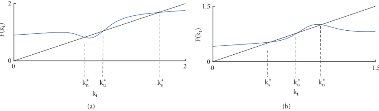
Figure 3: Parameter values𝑛 = 1.72, 𝛿 = .46, 𝑠𝑟 = .44, 𝛼 = 2.65, 𝛽 = 1.73, and 𝜌 = 8.82. (a) 𝑘∗𝑛 < 𝑘∗𝑢 < 𝑘∗𝑠 for𝑠𝑤 = .83 and 𝑐 = 2.95, (b)𝑘∗𝑠 < 𝑘∗𝑢< 𝑘∗𝑛for𝑠𝑤= .15 and 𝑐 = 7.5. 0 2.5 0 2.5 EN &(E N ) (a) 0 1.5 0 1.5 &(E N ) EN E02 E01 (b)
Figure 4: (a) Cases (a) in blue, (b) in green, and (c) in purple of Proposition 10. (b) Two coexisting attractors.
𝑘min. Assume 𝑘∗𝑛 ∈ (𝑘max, 𝑘min) to be a fixed point, then, considering Proposition 3 and being𝐹(0) > 0 and 𝐹(𝑘𝑡) > 0 ∀𝑘 < 𝑘max, it follows that up to two more fixed points may exist and, given the monotonicity of𝐹 for 𝑘 < 𝑘maxand𝑘 > 𝑘min, the number of fixed points determines their stability: if one fixed point𝑘∗𝑛ℎ exists, it is nonhyperbolic, while if two fixed points𝑘∗𝑠 and𝑘∗𝑢exist, they are, respectively, stable and unstable (in Figure 3 the cases𝑘∗𝑛 < 𝑘∗𝑢< 𝑘∗𝑠 and𝑘∗𝑠 < 𝑘∗𝑢< 𝑘∗𝑛 are depicted, respectively, in panels (a) and (b)).
The previous considerations are summarised in the fol-lowing proposition.
Proposition 10. Assume 𝐹 bimodal with 𝐹(𝑘𝑚𝑎𝑥) > 𝑘𝑚𝑎𝑥∨ 𝐹(𝑘𝑚𝑖𝑛) < 𝑘𝑚𝑖𝑛. Then map𝐹 has one fixed point 𝑘𝑚𝑎𝑥< 𝑘∗𝑛 < 𝑘𝑚𝑖𝑛with𝐹(𝑘∗𝑛) < 0. Moreover three cases may occur:
(a) no other fixed point exists;
(b) a nonhyperbolic fixed point𝑘∗𝑛ℎexists;
(c) two fixed points𝑘∗𝑠 and𝑘∗𝑢exist, with𝑘∗𝑠 stable and𝑘∗𝑢 unstable.
Therefore, a multistability phenomenon may occur (see Figure 4 panel (b)) and the model is able to explain why economies starting from different capital per capita levels may experience different long-run behaviours. This situation is depicted in Figure 5: starting from different initial con-ditions, two different attractors (in black and blue) may be reached.
Given the form of𝐹, an analytical study of the influence that parameters have on the loss of stability for the equilib-rium𝑘𝑛 is not possible. Therefore, we analyse this influence thanks to numerical simulations.
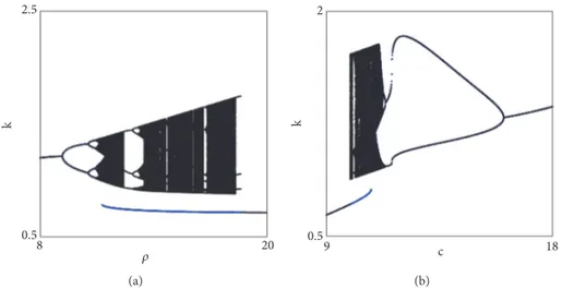
Figure 5(a) shows that the elasticity of substitution between production factors influences the generation of chaotic dynamics, as previous works demonstrated while considering economies in which capital is necessary for production. A different role is, instead, played by parameter 𝑐, which is related to labour productivity. Numerical simula-tions (an example is given in panel (b) of Figure 5) showed that fluctuations arise for low values of𝑐. Moreover when the productivity of labour is sufficiently high, the attractor is a fixed point, no cycles can be generated, and the value of capital per capita in equilibrium increases if𝑐 increases, since if𝑐 is sufficiently high and 𝐹 is bimodal, 𝐹(𝑘min) > 𝑘min. Given these results, an economic policy that increases the productivity of labour would push an economy out of boom and bust periods and increase the level of capital per capita in equilibrium.
5. Conclusions
In this work we introduced a technology that considers production possible even if the only input is labour, making criticism of the production functions previously used in economic growth models. We then investigated the long-run dynamics of the Solow-type growth model with differential
E 2.5 0.5 8 20 (a) E c 2 0.5 9 18 (b)
Figure 5: Bifurcation diagrams. Parameter values𝛼 = .2, 𝛽 = .4, 𝛿 = 𝑛 = .7, 𝑠𝑟= .8, and 𝑠𝑤= .1, initial conditions 𝑘min(black) and𝑘0= .02 (blue): (a) with respect to𝜌 for 𝑐 = 10; (b) with respect to 𝑐 for 𝜌 = 18.
savings between workers and shareholders, considering the function presented. Differently from previous works, we found that the origin is not a fixed point: when in the early stage of development an economy may produce only with labour, a positive evolution of capital per capita is observed. We showed that fluctuations may arise if the difference between saving propensities is sufficiently high. Moreover, we showed that an economic policy intended to increase labour productivity would push an economy out of boom and bust periods and increase the level of capita per capita in the equilibrium.
Data Availability
The data used to support the findings of this study are included within the article.
Disclosure
This paper did not receive specific funding and was per-formed as part of the employment of the authors to University of Macerata.
Conflicts of Interest
The authors declare that there are no conflicts of interest regarding the publication of this paper.
References
[1] R. M. Solow, “A contribution to the theory of economic growth,”
The Quarterly Journal of Economics, vol. 70, no. 1, pp. 65–94,
1956.
[2] T. W. Swan, “Economic growth and capital accumulation,”
Economic Record, vol. 32, no. 2, pp. 334–361, 1956.
[3] V. B¨ohm and L. Kaas, “Differential savings, factor shares, and endogenous growth cycles,” Journal of Economic Dynamics &
Control, vol. 24, no. 5-7, pp. 965–980, 2000.
[4] S. Brianzoni, C. Mammana, and E. Michetti, “Complex dynam-ics in the neoclassical growth model with differential savings and non-constant labor force growth,” Studies in Nonlinear
Dynamics and Econometrics, vol. 11, no. 3, 2007.
[5] S. Brianzoni, C. Mammana, and E. Michetti, “Nonlinear dy-namics in a business-cycle model with logistic population growth,” Chaos, Solitons & Fractals, vol. 40, no. 2, pp. 717–730, 2009.
[6] W. H. Masanjala and C. Papageorgiou, “The solow model with ces technology: Nonlinearities and parameter heterogeneity,”
Journal of Applied Econometrics, vol. 19, no. 2, pp. 171–201, 2004.
[7] C. Papageorgiou and M. Saam, “Two-level CES production technology in the solow and diamond growth models,” The
Scandinavian Journal of Economics, vol. 110, no. 1, pp. 119–143,
2008.
[8] S. Brianzoni, C. Mammana, and E. Michetti, “Variable elasticity of substituition in a discrete time Solow-Swan growth model with differential saving,” Chaos, Solitons & Fractals, vol. 45, no. 1, pp. 98–108, 2012.
[9] D. Cheban, C. Mammana, and E. Michetti, “Global attractors of quasi-linear non-autonomous difference equations: a growth model with endogenous population growth,” Nonlinear
Analy-sis: Real World Applications, vol. 14, no. 3, pp. 1716–1731, 2013.
[10] G. Karagiannis, T. Palivos, and C. Papageorgiou, “Variable elas-ticity variable elaselas-ticity of substitution and economic growth,” in New Trends in Macroeconomics, Diebolt, Claude, and C. Kyrtsou, Eds., pp. 21–37, 2005.
[11] S. Brianzoni, C. Mammana, and E. Michetti, “Local and global dynamics in a discrete time growth model with nonconcave production function,” Discrete Dynamics in Nature and Society, vol. 2012, Article ID 536570, 22 pages, 2012.
[12] S. Brianzoni, C. Mammana, and E. Michetti, “Local and global dynamics in a neoclassical growth model with nonconcave production function and nonconstant population growth rate,”
SIAM Journal on Applied Mathematics, vol. 75, no. 1, pp. 61–74,
2015.
[13] C. Azariadis and J. Stachurski, “Poverty traps,” in Handbook of
Economic Growth, P. Aghion, Ed., vol. 1, chapter 5, pp. 294–384,
Elsevier, 2005.
[14] A. K. Skiba, “Optimal growth with a convex-concave produc-tion funcproduc-tion,” Econometrica, vol. 46, no. 3, pp. 527–539, 1978.
[15] V. Capasso, R. Engbers, and D. La Torre, “On a spatial Solow model with technological diffusion and nonconcave production function,” Nonlinear Analysis: Real World Applications, vol. 11, no. 5, pp. 3858–3876, 2010.
[16] R. J. Barro and X. Sala-i Martin, Economic Growth, MIT Press, 2004.
[17] R. Sato and R. F. Hoffman, “Production Functions with Variable Elasticity of Factor Substitution: Some Analysis and Testing,”
The Review of Economics and Statistics, vol. 50, no. 4, p. 453,
1968.
[18] M. Prywes, “A nested CES approach to capital-energy substitu-tion,” Energy Economics, vol. 8, no. 1, pp. 22–28, 1986.
[19] P. Thompson and T. G. Taylor, “The Capital-Energy Substi-tutability Debate: A New Look,” The Review of Economics and
Statistics, vol. 77, no. 3, pp. 565–569, 1995.
[20] A. Jurgen, Technical change and the elasticity of factor
substitu-tion, vol. 147, Beitrage der Hochschule Pforzheim, 2014.
[21] F. Grassetti, C. Mammana, and E. Michetti, “Poverty trap, boom and bust periods and growth. A nonlinear model for non-developed and developing countries,” Decisions in Economics
and Finance, 2018.
[22] N. Paterson, Elasticities of substitution in computable general
equilibrium models. Working paper, Department of Finance
Canada, 2012.
[23] R. Klump and O. De La Grandville, “Economic growth and the elasticity of substitution: Two theorems and some suggestions,”
American Economic Review, vol. 90, no. 1, pp. 282–291, 2000.
[24] K. Miyagiwa and C. Papageorgiou, “Elasticity of substitution and growth: normalized CES in the Diamond model,” Economic
Theory, vol. 21, no. 1, pp. 155–165, 2003.
[25] N. Meager and S. Speckesser, “Wages, productivity and employ-ment: A review of theory and international data,” European
Employment Observatory, 2011.
[26] C. T. Tugcu, “How to escape the middle income trap: inter-national evidence from a binary dependent variable model,”
Theoretical and Applied Economics, vol. 1, no. 206, pp. 49–56,
2015.
[27] F. Tramontana, L. Gardini, and A. Agliari, “Endogenous cycles in discontinuous growth models,” Mathematics and Computers
Hindawi www.hindawi.com Volume 2018
Mathematics
Journal of Hindawi www.hindawi.com Volume 2018 Mathematical Problems in Engineering Applied Mathematics Hindawi www.hindawi.com Volume 2018Probability and Statistics Hindawi
www.hindawi.com Volume 2018
Hindawi
www.hindawi.com Volume 2018
Mathematical PhysicsAdvances in
Complex Analysis
Journal ofHindawi www.hindawi.com Volume 2018
Optimization
Journal of Hindawi www.hindawi.com Volume 2018 Hindawi www.hindawi.com Volume 2018 Engineering Mathematics International Journal of Hindawi www.hindawi.com Volume 2018 Operations Research Journal of Hindawi www.hindawi.com Volume 2018Function Spaces
Abstract and Applied AnalysisHindawi www.hindawi.com Volume 2018 International Journal of Mathematics and Mathematical Sciences Hindawi www.hindawi.com Volume 2018
Hindawi Publishing Corporation
http://www.hindawi.com Volume 2013 Hindawi www.hindawi.com
World Journal
Volume 2018 Hindawiwww.hindawi.com Volume 2018Volume 2018
Numerical Analysis
Numerical Analysis
Numerical Analysis
Numerical Analysis
Numerical Analysis
Numerical Analysis
Numerical Analysis
Numerical Analysis
Numerical Analysis
Numerical Analysis
Numerical Analysis
Numerical Analysis
Advances inAdvances in Discrete Dynamics in Nature and SocietyHindawi www.hindawi.com Volume 2018 Hindawi www.hindawi.com Differential Equations International Journal of Volume 2018 Hindawi www.hindawi.com Volume 2018