Essays on financial stability, credit dynamics and policy challenges

(1)

Doctoral Thesis

Essays on Financial Stability, Credit

Dynamics and Policy Challenges

This dissertation is submitted for the degree of

Doctor of Philosophy at the Sapienza Graduate Program in Economics (GPE)

Candidate

Advisor

Francesco Simone Lucidi

Prof. Giuseppe Ciccarone

Co-Advisor

Prof. Willi Semmler

(2)

(3)

Declaration of Authorship

I declare that this thesis titled, Essays on Financial Stability, Credit Dynamics and

Policy Challenges and the work presented in it are my own. I confirm that except

where specific reference is made to the work of others, the contents of this dissertation

are original and have not been submitted in whole or in part for consideration for any

other degree or qualification in this, or any other university. This dissertation contains

nothing which is the outcome of work done in collaboration with others, except as

specified in the text and Acknowledgements.

(4)

(5)

List of Figures

1 Contributions to the GFC . . . .

4

2 Financial and business cycles in US . . . .

5

1.1 Credit cycle filters . . . .

28

1.2 Credit cycle filters . . . .

29

1.3 Credit cycle filters . . . .

30

1.4 Credit Boom identification per country. The figure reports credit cycle

identified with only the Hamilton filter.

. . . .

32

1.5 Credit boom identification . . . .

33

1.6 Credit boom identification . . . .

33

1.7 Credit boom identification . . . .

34 1.10 Macro-financial variables around credit booms . . . .

34

1.8 Credit boom GFC . . . .

35

1.9 Lending margins around credit booms . . . .

36 1.12 EW Out-of-sample predictions

. . . .

41

2.1 δ(y) function based on the function arctan . . . .

51

2.2 α(y) function based on the function ˜

H

c

. . . .

52

2.3 Expansionary regime with positive inflation and output gap . . . .

55

2.4 Expansionary regime with positive inflation and output gap . . . .

55

2.5 Expansionary regime with tighter credit standards . . . .

57

2.6 Expansionary regime and tighter credit standards . . . .

57

2.7 Deflationary regime with negative output gap . . . .

58

2.8 Deflationary regime with negative output gap . . . .

59

2.9 Deflationary regime with tighter credit standards . . . .

60 2.10 Deflationary regime with tighter credit standards . . . .

61 2.11 Credit standards and credit growth . . . .

63

(8)

2.13 Credit standards shock, linear case . . . .

72 2.14 Credit standards shock, non-linear case

. . . .

72 2.15 Credit standards shock, non-linear case

. . . .

73 2.16 Credit standards shock, non-linear case

. . . .

74 2.17 Credit standards, risk management and bank’s supervision . . . .

78 2.18 MAR distribution . . . .

80 2.19 Scatter plots of credit standards and MAR

. . . .

83

3.1 Short-run effects of change in banking capital requirements . . . .

102

3.2 Time-series in the panel VAR . . . .

112

3.3 MPIX, capital ratio and macroprudential measures . . . .

113

3.4 MPIX, capital ratio and macroprudential measures . . . .

114

3.5 MPIX, capital ratio and macroprudential measures . . . .

115

3.6 Capital requirement shocks in Austria . . . .

115

3.7 Capital requirement shocks in Belgium . . . .

116

3.8 Capital requirement shocks in Germany . . . .

116

3.9 Capital requirement shocks in Spain . . . .

116 3.10 Capital requirement shocks in France . . . .

117 3.11 Capital requirement shocks in Greece . . . .

117 3.12 Capital requirement shocks in Italy . . . .

117 3.13 Capital requirement shocks in the Netherlands

. . . .

118 3.14 Capital requirement shocks in Portugal

. . . .

118 3.15 IRFs to CR shock in Austria

. . . .

119 3.16 IRFs to CR shock in Belgium . . . .

119 3.17 IRFs to CR shock in Germany

. . . .

120 3.18 IRFs to CR shock in Spain

. . . .

120 3.19 IRFs to CR shock in France . . . .

121 3.20 IRFs to CR shock in Greece . . . .

121 3.21 IRFs to CR shock in Italy . . . .

122 3.22 IRFs to CR shock in the Netherlands . . . .

122 3.23 IRFs to CR shock in Portugal . . . .

123 3.24 CR shock state-dependent local projections . . . .

124 3.25 CR shock state-dependent local projections . . . .

125 3.26 CR shock state-dependent local projections . . . .

126

(9)

List of Tables

1.1 Variable summary

. . . .

27

1.2 Credit cycle peaks above boom threshold

. . . .

31

1.3 Crisis periods . . . .

31

1.4 One-sample Kolmogorov-Smirnov test . . . .

32

1.5 Contingency Matrix

. . . .

36

1.6 EW credit boom buildups and financial vulnerable states

. . . .

37

1.7 EW and Global Variables . . . .

39

1.8 Out-of-sample analysis and multinomial logit . . . .

40

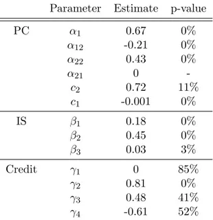
2.1 FIML estimation of the NLQ system . . . .

53

2.2 IV-Local projections . . . .

71

2.3 Banks involved in the IV . . . .

81

2.4 Mandatory auditors’ rotation scheme . . . .

82

2.5 First stage. Non-mandatory vs mandatory audit rotations . . . .

82

(10)

(11)

Introduction

” There are many more economic expansions than there are manias. But

every mania has been associated with the expansion of credit. In the last

hun-dred or so years the expansion of credit has been almost exclusively through

the banks and the financial system; earlier, nonbank lenders expanded the

supply of credit.”

Charles P. Kindleberger

”Unless we understand what it is that leads to economic and financial

instability, we cannot prescribe – make policy – to modify or eliminate it.

Identifying a phenomenon is not enough; we need a theory that makes

in-stability a normal result in our economy and gives us handles to control it.”

Hyman Minsky

The Global Financial Crisis (GFC) led to a deep and long-lasting economic

depres-sion worldwide. The financial meltdown that followed the subprime crisis in the United

States spread rapidly, with dramatic consequences for the well-functioning of the global

financial system. As a consequence, several countries experienced huge costs in terms

of output deterioration and unemployment rates. Between 2007 and 2010, the total

unemployment rate almost doubled in the United States (from 5 to 10 percent) and it

rose dramatically in the European GIIPS countries (from 7 to 17 percent). In the last

economies, the unemployment rate continued to rise sharply also as a consequence of

the sovereign debt crisis that started in the fall 2011.

Governments and taxpayers were hit by high social costs that threatened the

eco-nomic recovery of the following years. Rescue plans for the banking system involved

massive interventions to bailout credit institutions. In 2015, the Special Inspector

Gen-eral for the Troubled Asset Relief Program accounted that the US government’s total

commitment amounted to 16.8 trillion dollars while, according to the European

Com-mission State Aid Scorecard, in 2011, European governments allocated more than 3

trillion euros for banks’ bailout.

(12)

This evidence motivates the main research question addressed by this Dissertation:

How should the financial system oversight be organized in order to minimize social

costs?

The GFC took the immune defense system of advanced economies by surprise, as

policy makers had just ”mopped up” when the GFC erupted. Before this event, a large

part of central banks – by endorsing the so-called ”Greenspan doctrine”– believed that

the costs of any ex-ante intervention would have been larger than its benefits and that

financial crises were almost unpredictable. This ex-post approach was reflected in the

economic theory, as the mainstream framework at that time was almost absent of any

modelling structure allowing for financial market failures.

Things changed drastically at the dawn of 2008. Economists and scholars started

to investigate more in deep the main de-stabilizing mechanisms behind the financial

system, the link between the latter and the real economy, and whether it would be

possible to predict financial crises, or at least to attenuate their detrimental power

before eruption. This research agenda is nowadays the rule rather than the exception.

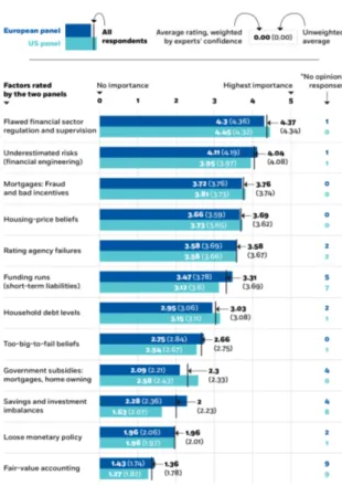
The Chicago Booth Review has recently conducted a survey among economists,

asking what were in their opinion the main causes of the GFC. Each of the twelve

items in Figure 1 reflects, not just personal beliefs, but also different topics currently

addressed by economic research. However, the larger part of both U.S. and European

economists believe that the main factor that exacerbated the effects of the GFC was

the lack of regulation and supervision of financial markets.

In the aftermath of the GFC, a new set of rules and policy tools – embedding also

an ex-ante perspective– was activated in order to make the system more resilient to

financial meltdowns. Improving the understanding of how risk-taking spreads across

fi-nancial actors, in general, and how to monitor the exposure to risk of credit institutions,

in particular, have become a primary concern that falls into the scope of the so-called

macroprudential policy. The larger part of central banks, governments, national and

international financial supervisory authorities conceive now the macro-approach to

fi-nancial regulation as an independent pillar of their policy mandate. However, after a

decade of research, many doubts about the functioning, the implementation, the

ef-fectiveness and the impact of macroprudential measures continue to feed the policy

debate.

The identification of a single system-wide risk measure that can support policy

makers to steer macroprudential tools remains one of the unsolved challenges. Powerful

(13)

indicators may help to provide policy makers with timely (ex-ante) warning signals, but

these signals, in their turn, depend on how sensitive the definition of financial stability

is, and ultimately on the empirical identification of the financial cycle. Figure 2 shows

the business (GDP) cycle in the United States and its financial cycle, according to the

estimation of the Bank of International Settlements (BIS). The financial cycle is obtained

as co-movements in the medium-term dynamics of credit and property prices. The

graph shows that all financial crises origin at the peak of the financial cycle and, most

importantly, that when recessions coincide with a contractionary phase of the financial

cycle GDP drops more than in other recessions. This is why, over the last decade, the

benchmark measures monitored by the authorities to gauge the buildup of risks overtime

relate, one way or another, to credit dynamics. Moreover, the availability of both

brand-new datasets and more sophisticated econometric tools has given the opportunity to

build a solid empirical evidence suggesting that excessive credit growth actually played

a central role in determining the severity of the GFC and that credit boom-bust cycles

dramatically affect the real economy through amplification mechanisms.

The three chapters of this dissertation add to the debate on the subject matter by

providing a theoretical model highlighting the relevance of credit dynamics for policy

makers, as well as new empirical insights about the control of credit dynamics and the

conduct of macroprudential policy.

The idea of considering credit as a key driver of financial crises and/or as an

ampli-fying engine of exogenous shocks is not new in the literature. This view, –particularly in

the pioneering contributions by Fisher (1933), Minsky (1977) and Kindleberger (1978)–

looks at the credit dynamics as an endogenous force that is prone to generate

instabil-ity. Once speculative opportunities are present in the system, prolonged increases in

the demand for goods and financial assets transmit themselves to prices. Higher prices

means new profit’s opportunities that attract further investors. This positive feedback

is characterized by the ”euphoria” of economic actors and the boom starts to develop.

The so-called ”mania” phase comes as people’s judgment on speculation for profits does

not reflect the economic fundamentals of the underlying goods or assets. As booms are

generally fed by expansions of banks’ credit, the latter is taken as an indicator of the

temperature of systemic risk.

In line with this theoretical perspective, Chapter 1 investigates the anatomy of credit

booms –which are defined as statistical events obtained from the filtering of credit’s

(14)

Figure 1: Source: ”What contributed most to the financial crisis?”, The Chicago Booth Review

time-series– and their connections with financial crises. Furthermore, the chapter

ex-plores the relative power of macro-financial measures to provide policy makers with

anticipatory warning signals relative on the occurrence of credit events. A correct and

timely identification of these events motivates the setup of ex-ante measures addressing

the control of credit dynamics. The latter can be carried out directly or indirectly, in

the sense that policies can also influence the attitude towards risk, which leads credit

to grow faster, rather than limit the volume of credit itself. Direct measures are, for

instance, reductions in the loan-to-value ratios (LTV) or in the debt-to-income ratios

(DTI) that banks set to borrowers, or limits on concentration and exposures. As for

indirect measures, authorities can set capital ratios, or counter-cyclical capital buffers

to banking institutions. However, these measures are not a free-lunch. Though

reduc-ing systemic risk is a benefit for financial stability, a policy that damps credit growth

may trigger side-effects, like credit crunch and fire-sales that, if the economy is in a bad

(15)

Figure 2: Financial and business cycles in US. Source: ”Characterising the financial cycle: don’t lose sight of the medium term!”, BIS Working Papers 380.

shape, may threaten the recovery.

The theoretical above-mentioned underpinning and the empirical evidence presented

in Chapter 1 suggest that economic break-downs accompanied by financial unbalances

are deeper and readjustment processes are long-lasting than normal recessions, so that

the standard policy approach might be insufficient to put the economy back on a

sta-bility path. As in the case of the GFC, central banks might be forced to implement

unconventional tools to stimulate economic recovery. Yet, the fact that the

mecha-nisms behind financial instability underlie a nonlinear behavior of the economy is also

an hardship to face in the ex-ante policy approach.

Chapter 2 addresses this issue, both theoretically and empirically. On the theoretical

side, nonlinearities represent a severe challenge to central banks’ monetary policy. Here

the (nonlinear) credit dynamics becomes a policy target to monitor financial stability,

inasmuch as the central bank is allowed to lean against the buildup of financial

unbal-ances by increasing the policy rate when credit overheats. Against this background, this

chapter presents a small scale nonlinear quadratic model, where credit flows and credit

spreads enter the reaction function of the central bank and where implied feedback

effects impact the overall adjustment path of the economy. The feedback effects are

thought as representing credit standards that the banking sector set to private

borrow-ers. Policy decisions in two business-cycle regimes are then studied from the perspective

of relaxing or tightening credit standards.

The chapter also presents a non-linear estimation of the macro impact of policy

changes to credit standards, conceived as arising from a structural innovation to banking

supervision. On the overall, the results confirm that the impact of supervisory measures

(16)

is stronger when real activity is contracting. This leads to the conclusion that, in that

economic regimes, policy targeting risk-taking can be relatively costly. Intuitively this

result is not surprising, as banks’ risk-sensitivity tends to be lower in good times and

higher in bad phases.

This result raises new questions about the effectiveness of indirect ex-ante measures.

For instance, prudential capital regulation implies that banks are asked to improve some

capital ratio of their balance sheets. Banks can meet higher requirements by lowering

their (risky) exposure, or by issuing new equity (retaining earnings). However, if banks’

risk-perception is high and financial markets are stuck, so that it becomes burdensome

to rise new equity, banks will be forced to shrink the supply of new loans. This result

can be very unpleasant for policy makers if the economy is recovering from a recession.

Chapter 3 deepens this issue by studying empirically the macro impact of capital

measures in Euro-Area countries under different economic regimes. Though capital

regulation in Europe mostly comes from the implementation of Basel’s international

agreements, the narrative of country-specific capital rules advocates to analyze about

the effects of unexpected changes in that regulation. Capital requirements are hence

studied in the form of policy innovations. By following the economic theory and the

empirical evidence, the analysis assumes that a capital requirement shock increases the

capital ratio of the banking system and it makes the equity a relatively costly source of

funding for banks, while increasing lending rates. In the final part of this chapter,

state-dependent responses to capital requirement shocks are shown to confirm that bank credit

falls more during contractions, with amplifying negative effects on the macroeconomy.

The results I obtain in this Dissertation suggest that financial supervision, in general,

and capital measures, in particular, can actually exacerbate credit procyclicality. The

policy message of the last two chapters is that macroprudential policies might be

detri-mental if hurriedly implemented in regimes of financial or economic turmoils. The first

chapter shows however that the predictive power of real-time information in detecting

systemic risks’ buildups is a good guideline for policy makers. This information provides

anticipatory signals that can help to distinguish credit growth reflecting adjustment to

economic fundamentals from the one which reflects increasing appetite for risks. From

this perspective, an ex-ante intervention limiting the tendency of the banking system

to embrace new risks by extending lending activities becomes desirable.

(17)

Chapter 1

Real-time signals anticipating

credit booms in Euro Area

countries

This paper identifies credit booms in 11 Euro Area countries by tracking private loans

from the banking sector.

The events are associated with both financial crises and

specific macro fluctuations, but the standard identification through threshold methods

does not allow to catch credit booms in real time data. Thus, an early warning model

is employed to predict the explosive dynamics of credit through several macro-financial

indicators. The model catches a large part of the in-sample events and signals correctly

both the global financial crisis and the sovereign debt crisis in an out-of-sample setting

by issuing signals in real-time data. Moreover, while tranquil booms are driven by

global dynamics, crisis-booms are related to the resilience of domestic banking systems

to adverse financial shocks. The results suggest an ex-ante policy intervention can avoid

dangerous credit booms by focusing on the solvency of the domestic banking system and

financial market’s overheating.

1.1 Introduction

The legacy of the Global Financial Crises prompted a widespread debate about ex-ante

policy, that is an early intervention of policymakers during economic expansions, in

order to make the economic system more resilient to adverse financial shocks and to

avoid expensive ex-post measures, like bank bailouts or unconventional policies during

downturns. This paper provides empirical evidence about credit booms and a strategy

(18)

to provide early signals to introduce an ex-ante intervention with focus on the dynamics

of credit of several Euro Area countries. A preliminary analysis confirms the

well-established findings that credit booms are frequent events and that they are strictly

related with states of macroeconomic and financial instability. These facts motivate to

build an early warning model which signals coming credit booms and shows whether

those signals are useful indicators of future crises.

A widespread empirical literature highlights the importance of the financial cycle

in triggering long-lasting real crises and the potential amplification mechanisms that it

can engender, in particular through banking crises (

Borio

[

2014

]). Yet, many authors

stressed the pre-emptive power of credit and asset prices in signaling systemic financial

risks (

Borio and Lowe

[

2002

]). Important works like

Jord`

a et al.

[

2015

,

2013

];

Schular-ick and Taylor

[

2012

] build long-run analyses to study the historical determinants of

financial crises. They find that credit growth is a key predictor of financial crises and

suggest that credit aggregates are superior policy indicator to pursue financial stability.

Mendoza and Terrones

[

2012

,

2008

] (henceforth MT) find credit booms are source of

economic turbulence and identify these as unusual expansions in the cyclical component

of private credit.

This paper identifies credit booms through a threshold method like in MT, then it

employs an early warning model (EW henceforth) in the same spirit of

Schularick and

Taylor

[

2012

]. However, three main differences characterize the analysis here. First,

credit booms are identified exploiting real-time information exclusively. Second, the

EW predicts states that anticipate the starting date of the event, that is credit-boom

buildups. Third, in line with further works, the EW evaluation criteria are based on

the signaling approach — developed by

Kaminsky and Reinhart

[

1999

] and extended in

Alessi and Detken

[

2009

,

2011

]— to provide signals subject to policy preferences. This

strategy accounts for the relative aversion of policymakers against Type I errors (not

issuing a signal when an event is imminent) and Type II errors (issuing a signal when

no event is imminent). The final goal is to compute an optimal threshold to qualify the

predicted probability estimated through the EW and to test its predictive power.

Furthermore, the EW developed in this paper takes into account the different

ad-justment processes of macro variables during crisis states, i.e. the so called crisis and

post-crisis bias (

Bussiere and Fratzscher

[

2006

]). In the same spirit, a multinomial logit

model is implemented also to distinguish credit booms that are followed by crisis from

tranquil credit booms. The latter provides useful insight to policymakers to distinguish

(19)

those booms that reflect adjustment of credit to economic fundamentals.

This work relates to recent EW advancements such as the work of

Sarlin

[

2013

], which

emphasizes the role of policymakers’ preferences in the optimal threshold determination.

Also it relates to

Duca and Peltonen

[

2013

] and

Behn et al.

[

2016a

] who identify systemic

events through a financial stress index and find that global variables have a greater

impact with respect to the domestic dimension. Similar analyses can be found in

Behn

et al.

[

2013

] and

Behn et al.

[

2016b

], showing that this model can help policymakers to set

counter-cyclical capital buffers and to gauge the benefits of capital ratio macroprudential

measures through the estimated probability of having a financial crisis. Yet, the results

in this paper are presented so to allow a comparison with the latter.

A recent contribution by

Richter et al.

[

2017

] shares many similarities with this

paper. However, here credit-boom thresholds are set to identify large displacements

from the long-run trend, consistently with the theoretical intuition that credit booms

are out-of steady-state phenomena (

Brunnermeier and Sannikov

[

2014

]). Moreover, the

boom-threshold factor here is based on a real-time standard-deviation of the credit

cyclical component, so that the EW might be used for actual predictions or

out-of-sample analyses. However, one drawback with respect to

Richter et al.

[

2017

] is that,

due to a shorter sample, the logistic EW cannot be used to distinguish bad from good

credit booms directly. Alternatively, the paper provides estimates of tranquil and bad

credit booms through an multinomial logit. The latter allows to highlight new insights

about the nature of credit booms which are at odds with

Richter et al.

[

2017

].

Though the research have extensively deepened the relevance of credit cycle and

its relationship with the real economy, the role of credit booms for policy purposes is

much more controversial. This paper encourages EA’s policymakers to use real-time

EW models to set ex-ante interventions targeting the credit cycle. Besides to confirm

well-known results of the literature and that real-time EWs provide accurate signals

anticipating credit booms, the paper adds also another important result. Dangerous

credit-boom buildups can be distinguished from tranquil ones, inasmuch the former are

significantly characterized by a low capitalization of the domestic banking system and

a high stock prices growth.

The paper is structured as follows: Section 1.2 defines credit booms and

filter-ing techniques to identify them in a sample of EA countries. Also, an event analysis

shows the relationship between credit booms and macro-financial patterns, while a

fre-quency analysis shows whether these booms are related with financial crises. Section

(20)

1.3 presents the logistic EW and its evaluation criteria. Section 1.4 reports baseline

results and further analysis. Section 1.5 collects some concluding remark.

1.2 Credit filters, booms and financial instability. Stylized

facts and macro implications

There are several arguments about financial instability drivers, but a consistent part of

the literature relies on the private credit dynamics as a broad measure of the financial

cycle. From an ex-ante perspective, the salient part of its dynamics is linked with

buildup phases, when a consistent deviation of private credit from its long-run trend

is observed. In this paper credit booms are identified through several strategies, but

it follows as a benchmark the one proposed in MT. The latter relies on a threshold

method: more specifically, it takes significant and positive deviation of private credit

from its long-run trend. Thus, the credit boom is a time period where the following

condition holds:

l

i,t

≥ φσ(l

i,t

)

(1.1)

where l

i,t

is the cyclical component of the private credit for country i at time t, σ(l

i,t

)

is its standard deviation and φ is the boom threshold factor. The latter is set equal to

1.65 because the 5% tail of the standardized normal distribution satisfies P (l

i,t

/σ(l

i

) ≥:

Q1.65) = 0.05. However, this specific φ’s calibration is subject to hypothesis testing of

normality of the cyclical components that are discussed next.

Three points in time are defined to identify the event: the peak (ˆ

t), the starting date

(t

s

) and the ending date (t

e

). The peak is the date of the contiguous dates set satisfying

the (1) that shows the maximum difference between l

i,t

and φσ(l

i

). The starting date of

the credit boom is defined as a date t

s

_{< ˆ}

_{t yielding the smallest difference |l}

i,t

− φ

s

σ(l

i

)|.

The ending date is a date t

e

> ˆ

t yielding the smallest difference |l

i,t

− φ

e

σ(l

i

)|. The

start and the end thresholds, φ

s

_{and φ}

e

_{respectively, for simplicity are set both equal to}

one, although robustness checks have been implemented without changing the results.

The thresholds setting is so that φ

s

= φ

e

< φ, and the duration of the credit boom is

obtained from the difference t

e

−t

s

_{. Notice that, following this definition, the whole event}

is described by both the upswing and the downswing of credit deviation. Therefore, in

real-time data such an event can be identified only once the credit cycle collapses, i.e.

ex-post. Although the credit boom’s identification of this section relies on this definition,

(21)

the EW in next section focuses only on the buildup phases of the event, so as to generate

timely signals to implement an ex-ante policy intervention.

In MT the credit-cycle component of the credit is obtained through a two-sided

Hodrick and Prescott

[

1997

] (HP) filter with smoothing parameter set equal to λ =

1600 for quarterly data. However, the use of the HP filter has been recently criticized

in

Hamilton

[

2018

]. The Hamilton filter regresses an actual observation on its past

observations for a given time horizon, so that the cyclical component is just the error

term coming from this regression. In other words, the long-run trend is conceived as all

of what can be explained using historical data. With two-sided HP, instead, cycle-waves

are shaped on the whole information available in the sample and forecasts would be then

flawed by this extra-information.

In

Richter et al.

[

2017

] the use of the Hamilton filter is central for the identification

of credit booms. However,

Drehmann and Yetman

[

2018

] find that de-trended

credit-to-GDP ratio obtained through one-sided HP filter, with an higher smoothing parameter

λ = 400000, outperforms many other measure of credit gap in predicting financial crisis.

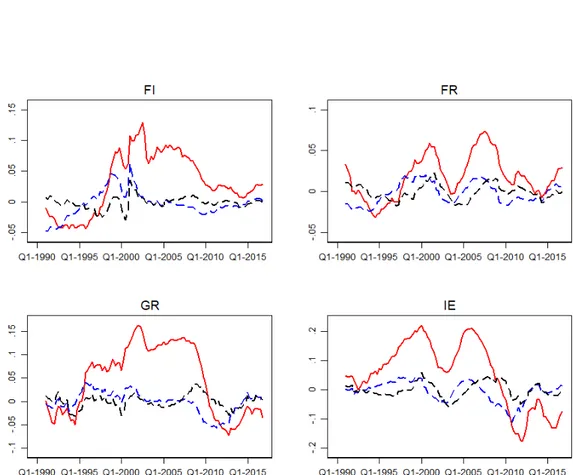
Figures 1.1-1.3 show the series of the cyclical component of the (log) CPI-deflated

credit of the banking system obtained through the three filtering techniques.

1

These

are obtained in a sample of 11 Euro-Area countries (EA)

2

for the largest time span

available at quarterly frequency (1974:Q1–2018:Q1) in order to minimize the loss of

information and reported from 1990:Q1. The Hamilton filtered cycles (red lines) are

the one presenting more amplified swings.

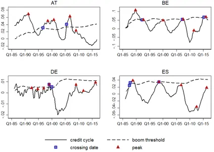
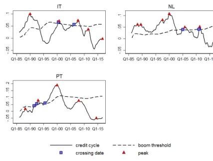
Table 1.2 reports peak-dates of credit cycle for the Hamilton, one-sided and two-sided

HP filters. Peaks are identified by employing the

Harding and Pagan

[

2002

] algorithm

with a minimum length of each phase of four quarters. The number of cycle-peaks are

31, 9 and 22 respectively. Notice that the latter do not identify always a credit-boom

event. All the filters indicate credit-cycle peaks in the around of the dot-com bubble

(1998–2002) for the largest part of EA countries. The Hamilton and the two-sided HP

filters peak in period 1990–1992 in Finland, France and Italy. The latter indicate also

a peak in the around of the global financial crisis (2005–2009) in almost all countries of

the sample.

1_{The smoothing-parameters are λ = 400000 for one-sided and λ = 1600 for two-sided HP filters.}

The Hamilton filter projection horizon of 20 quarters to reflect the long duration of credit cycles as in

Hamilton[2018] andDrehmann and Yetman[2018].

2_{Austria (AT), Belgium (BE), Finland (FI), France (FR), Germany (DE), Greece (GR), Ireland}

(22)

Before to identify credit-boom events, it is safer to test the assumption that credit

cycles come from normal distributions, which justifies to calibrate the boom-threshold

factor φ = 1.65. The (one-sample) Kolmogorov-Smirnov test indicates to what extent

the observed credit-cycles deviate from a normal distribution, so that if the null

hy-pothesis is true this deviation is likely small. Table 1.4 reports the D-statistic

3

and the

relative p-values for credit cycles obtained with the three filters for each country in the

sample. In most cases a failure to reject the null hypothesis is recorded. Specifically, in

all countries when credit cycles are obtained through one-sided HP filter. In 9 countries

in the case of the two-sided HP and 8 in the Hamilton filter case.

By applying the threshold method of MT, the Hamilton filter is the one that identifies

more credit booms (20 events), followed by the two-sided HP filter (18 events) and the

one-sided HP filter (only 8 events). Though the two-sided filter by using past, present

and future information provides a genuine representation of the long-run trend, the

resulting credit cycles would be less useful for forecasting purpose. Therefore, for the

purpose of predicting excessive credit dynamics through the EW model, in what follows

the Hamilton-filtered credit cycle will be used as benchmark to identify credit-boom

events. However the one-sided HP is taken as benchmark for Germany, Spain, Greece

and Italy to meet the assumption of normality of the boom-threshold factor.

1.2.1 Stylized facts on credit dynamics within the Euro Area

In this subsection credit booms are identified in order to study their cross-country

frequency and the behavior of macro-financial variables in the neighborhood of the

event. The sample in object collects quarterly data for 11 EA countries from 1991:Q2

to 2017:Q4.

The advantage of this sample is twofold: on the one hand, there are

enough post-2008 observations to analyze the behavior of the main macro variables

in the aftermath of the global financial crisis. On the other hand, since the focus is

on countries adopting Euro convergence criteria, periods of exchange rates overheating

are excluded for the most part of the sample period. The time-series used for the

identification is the cyclical component of real private credit (deflated by the CPI)

sourced by the Bank of International Settlements (BIS), that captures both loans and

debt security instruments. In principle, there are two versions of this series: one is the

private credit from domestic banking systems, the other is the private credit from the

3_{This indicates maximal absolute difference between the observed and the normal cumulative relative}

(23)

whole financial sector. These two series share a similar path up to the beginning of

the global financial crisis, then the former slows down and the latter increases rapidly.

They track almost the same boom episodes, but since the analysis keeps a close watch

on banking crises and since EA countries are mostly bank-based, the focus will be on

the first one.

4

Overall, 20 credit booms are identified, ranging from 1 to 3 episodes per country with

an average duration of 8 quarters. Nine countries experienced a credit-boom between

1996:Q1 and 2000:Q1, before the collapse of the dot-com bubble, while five between

2007:Q1 and 2008:Q3, before the collapse of Lehman Brothers.

5

The sample average

standard deviation of credit’s cyclical components, σ(¯

l), is 3% above the trend.

The event analysis shows cross-country means and medians of macro-financial

vari-ables (Figures 1.7–1.10). Of course, there is no causal interpretation for these figures,

but they show that characteristic patterns around credit booms belong to both the

time and the cross-sectional dimension. For the large part of the variables, average

dynamics are not influenced by outliers since there are no significant differences from

their respective median dynamics. The figures show a five-years window (21 quarters)

centered at the peak of the credit boom (ˆ

t is normalized to t = 0). Figure 1.7 shows real

private loans and real GDP cycles. This suggests that credit booms are associated with

a specific pattern of the business cycle across countries, which is the same regularity

that MT find for advanced economies during the period 1960-2010.

Panel (a) shows that, on average, the credit cycle is symmetric around the peak and

that it starts to cross the trend about a year and an half before the farthest deviation.

The average peak is about 7% above the trend. In the following quarters, on average,

the credit falls about 2 points below its trend. Panel (b) shows that the GDP cycle rises

suddenly during the buildup of the boom, about 2% above the trend, and drops up to

1 point below it during the downswing. Notice that, less than 50% of credit booms are

concomitant to GDP booms tracked through the same threshold method. However, the

business cycle around the booms reveals also several differences among countries.

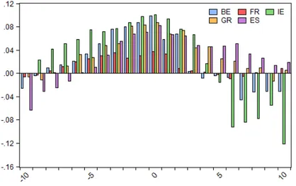
Figure 1.8 shows country-specific events occurred during the period 2007:Q1-2008:Q3,

before the Lehman Brothers collapse. Also in this case the peak of the boom is

cen-tered at t = 0. Credit increases rapidly in Ireland, Greece and Belgium, while Spain

4

By using loans from the whole financial sector three more episodes are identified in Portugal and an additional event in other two countries although they last no more than three quarters.

5_{Dot-com bubble: AT, ES, FI, FR, GR, IE, IT, NL and PT. Global financial crisis: AT, ES, FI, FR}

(24)

and France experience a slower buildup phase (Panel a). Belgium and Ireland are also

those countries that experience a severe bust phase up to 12 points below the trend.

Almost all countries present large fluctuations of real GDP cycle, but Spain and Greece

show an asymmetric pattern after the peak. Moreover, apart from Spain, all countries

experience a severe GDP fall about 2% below the long-run trend within the two years

that follow the peak.

Figure 1.9 presents the event analysis for lending margins of EA banking systems.

These credit spreads indicate bank’s profitability, and are calculated as the difference

between the average lending rates and the average deposit rate to both households

and non-financial corporations (NFCs henceforth). Figure 1.9 is split between lending

margins to new loans/deposits and outstanding loans/deposits. Since these data are

available from 2003, we can include only credit booms related to the global financial

crisis and the sovereign debt crisis.

6

_{The analysis shows an average downward pattern}

before the peak and a sudden increase after the boom. However, margins on outstanding

amounts have a deeper downward tendency also after the peak, while, margins on new

businesses are flatter before the boom and jump suddenly at the peak date. Indeed,

margins on new businesses are less sluggish and capture recent developments in bank

interest income in a more timely fashion.

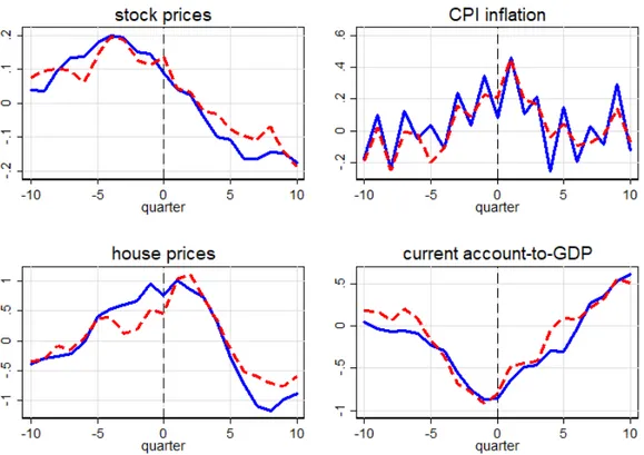
7

Figure 1.10 shows the event analysis for other macro variables. The cycles of current

accounts as percentage of the GDP, a stock index (deflated by the CPI), an house price

index and the CPI inflation rate (quarter-on-quarter). The current account displays a

deficit greater than 0.8% of GDP at the peak, but it gradually turns to a surplus up to

0.6% of GDP. The house price index records on average a 10% increase at the peak and

a fall in the downswing about the same extent, showing a pattern similar to that of real

credit cycle. The stock price index shows a similar pattern to the real GDP cycle: it

increases about 20% during the buildup of the boom and it falls in the after the peak on

a similar extent. The inflation rate has not particular tendency around the event since,

showing only an above-trend pattern around the quarters close to the peak at median

level.

Another important question is how frequently credit booms relate to crisis states.

To study this relationship one need a clear definition of crisis states that clearly

distin-guishes financial from other types of crises. This paper follows the classification made

6

Specifically, the following countries are involved (peak date): Belgium (2008:Q1), France (2008:Q4), Greece (2009:Q1), Ireland (2008:Q1), Italy (2011:Q3), The Netherlands (2011:Q2), Spain (2007:Q3).

7

(25)

in

Duprey et al.

[

2017

], which identify systemic financial stress dates using a

Markov-switching model selection. One reason to use it is that the model captures on average

100% of the banking crises identified by

Laeven and Valencia

[

2013

] that is generally

accepted as benchmark for crises identification. More specifically, the model selects

financial stress episodes that are associated with prolonged declines in real economic

activities. These are defined as at least six consecutive months of negative annual

in-dustrial production growth concomitant to a decline in real GDP during at least two

quarters. Moreover, the model allows to construct an EU crisis simultaneity index that

preserves cross-country comparability. Crises dates are reported in Table 1.3. The

fre-quency analysis reveals that 70% of credit booms are associated with crisis states, of

which 80% relates to banking crises, while the rest to equity crashes in the private

sec-tor. Almost 70% of credit booms start prior to the crisis, ranging from 2 to 9 quarters

before. However, 30% of these do not end up in crises and they have a maximum

dura-tion of four quarters. Finally, on average, countries have more than 50% of probability

of experiencing a credit boom (that in MT definition includes also credit downswings

after a peak) once the starting threshold is crossed.

Summarizing, the analysis shows that banking credit booms in the EA are associated

with specific patterns of many macro-financial variables. On average the event starts

with a surge in the cyclical component of GDP, house price indexes, stock indexes,

increasing deficits in current accounts and declining lending margins during the buildup

phases, followed by an opposite pattern during credit downswings. These results confirm

and reinforce MT analysis, notwithstanding their fluctuations result more accentuated

around the peak, probably due to a larger sample — both in time and cross-sectional

dimensions — that allows them to track many other episodes.

1.3 An Early Warning system to identify the booming

na-ture of the credit cycle

This section focuses on the left-hand side of credit boom event as in Figure 1.7. The

goal is to obtain a signal that predicts the buildup of the boom in order to provide

policymakers with timely information to setup an ex-ante intervention. One caveat of

MT’s method is that a credit boom is qualified as such only when the credit cycle crosses

its standard deviation times a threshold factor. This method, in fact, is such that credit

cycle has to be un-normally far from its long-run trend, so as to avoid concerns about

(26)

credit dynamics every time this is above its growth path, possibly also in a good shape.

However, as the event analysis has shown, the credit cycle crosses its boom threshold

about an year before it collapses, therefore contingent pre-emptive signals can be policy

relevant. The setup of this section is a multivariate logistic EW model that assesses the

power of several variables in predicting credit boom buildups. This section also tests

the ability of the EW model to catch credit booms states rather than financial crisis

states. As not all credit booms turn into financial crises, this can be a potential source

of bias for policy makers that should be taken into account.

Thus, the same model is estimated for two different dependent dummy variables.

Since the latter are binaries, the probability estimated on the left-hand side of the model

is a non-linear function of the regressors on the right-hand side. The logistic model is

described by the following equation:

P (Y

i,t

= 1) =

e

αi+βiXi,t0

1 + e

αi+βiXi,t0

(1.2)

The left-hand side variable is the probability of being in a given state for country i at

time t. On the right-hand side, α

i

catches the unobserved country-heterogeneity, while

X

i,t

is a vector containing macro-financial regressors. The latter consists of growth rates

of macro financial variables and other predictors in level.

8

The latter consists of real

GDP, real credit from the banking system, real credit from all financial institutions,

the CPI inflation, an house price index, a stock price index, the consolidated banking

capitalization (defined as equity on total assets in levels), an average of lending rates and

lending margins of consolidated banking systems. Alternatively, by splitting the real

credit from the whole financial system, the model is regressed on credit to households

and credit to NFCs.

All the specifications allow country fixed effects. The estimation does not include

time dummies that would account for heterogeneity in crisis probability over time.

Notice that, although time dummies would improve the ex-post fit of the model catching

the global time factors— that drive the left-hand-side of the logit— they are unknown

ex-ante. Thus, time dummies add little help to the EW evaluation, especially in the

out-of-sample forecasting.

9

However, since the global financial crisis affected almost all

8

As pointed out inBehn et al.[2013], Year-on-Year growth rates have much more predictive power than Quarter-on-Quarter growth rates. The analysis here takes YoY rates as benchmark and QoQ for robustness checks.

9

(27)

countries in the sample, robust standard errors clustered at quarterly level are employed

in order to account for potential correlation in the error terms.

As clarified above, the first model specification uses two main dependent variables

representing credit boom buildups and financial vulnerability states. As in

Behn et al.

[

2016a

], the latter is a binary variable that equals one between 7 and 12 quarters prior to

a systemic crisis and zero otherwise. Again, systemic crisis states are identified following

Duprey et al.

[

2017

]. That way, the dependent variable allows to catch vulnerable states

early enough without loosing accuracy. This is set so as to leave sufficient time to

policymakers to implement adequate actions. In the same spirit, the second dependent

variable anticipates credit downswings, and it equals one between 4 and 9 quarters

before the boom threshold is crossed. Thus, on average, this dummy equals one between

7 and 12 quarters before credit cycle collapses after having crossed its boom threshold.

As shown in the previous section, those phases are concomitant to the worsening of

macro conditions and in many cases they are associated to financial crises. The credit

boom dummy is chosen among four main specifications that take different upper bounds

as reference points: the peak, the starting date and the whole event rather than the

threshold-crossing date. However, the latter is preferred for two main reasons: first,

it allows to avoid overlaps with crisis states and, second, on average it corresponds to

the financial vulnerability dummy every time a financial crisis is anticipated by a credit

boom.

Moreover, the estimation avoids the post-crisis bias that may arise when the

depen-dent variable does not discriminate between tranquil periods (when economic

funda-mentals are sustainable) and crisis states (when macro series are much more volatile).

Following

Bussiere and Fratzscher

[

2006

], this potential source of bias is addressed first

by excluding quarters of crisis states from the estimation and then by performing a

multinomial logit as robustness check. In the latter the dependent variables are

speci-fied so as to distinguish both tranquil, vulnerable and crisis states (see Section 1.4).

1.3.1 Model evaluation

The predictive ability of the EW models are measured following several evaluation

criteria. The underlying idea is to compare the predicted probability with the actual

outcome in the data, by defining a threshold above which the former signals that an

event is about to occur. The signaling approach consists in finding this optimal threshold

τ ∈ [0, 1], defined as a percentile of the distribution of predicted probability.

The

(28)

latter,

_{P (Y}

\

_i,t

_{= 1) is transformed into a binary predictor d}

_P

_j,t

_{, that equals one when the}

continuos predictor crosses the threshold and zero otherwise. Thus, signals issued by

this binary predictor are compared with the actual outcome, C

i,t

, that equals one for

effective realizations observed in the data and zero otherwise. The latter has to be

interpreted according to which dependent variable is considered. In the case in object,

C

i,t

equals one if country i experiences a crisis within the following 7-12 quarters (i.e.

from t + 7 to t + 12) and zero otherwise for the financial vulnerability dummy, while,

C

i,t

equals one if the credit cycle crosses the threshold within the following 4-9 quarters

(i.e. from t + 4 to t + 9) and zero otherwise for the credit boom dummy.

Each observation can be then classified in a contingency matrix reported in Table

1.5. There is a true positive (T P ) when the model issues a signal and a realization in

the actual class is observed, a false positive (F P ) when the model issues a signal that

does not correspond to a realization in the actual class, a false negative (F N ) when the

model does not signal a realization which instead is observed in the actual class, and

a true negative (T N ) for an observation to which corresponds both no signal and no

realization in the actual class.

In order to find the optimal threshold, τ , the policymakers preference has to be set.

The latter can be thought as a parameter µ ∈ [0, 1] denoting the relative aversion to

Type I errors (i.e. the rate of missed realizations, T

1

(τ ) = F N/(T P + F N ) ∈ [0, 1]) and

to Type II errors (i.e. the rate of false alarms, T

2

(τ ) = F P/(T N + F P ) ∈ [0, 1]). In

general, µ is grater than 0.5, reflecting the fact that policymakers are more willing to

issue a false alarm than missing a realization because crises are costly. In particular, in

the baseline specification µ = 0.85, but other calibrations are set as robustness checks.

Therefore, the optimal threshold has to minimize the following loss function depending

on the two errors (T

1

and T

2

) weighted for the policymakers’ preference (µ):

L(µ, τ ) = µP

1

T

1

(τ ) + (1 − µ)P

2

T

2

(τ )

(1.3)

As in

Sarlin

[

2013

], equation (1.3) assumes that policymakers are concerned about the

absolute number of misclassifications, so as to account for the relative frequencies of the

actual class, which are P

1

= P (C

i,t

= 1) and P

2

= P (C

i,t

= 0).

A crucial evaluation instrument is the so called usefulness of the EW that can

be obtained through the loss function.

Alessi and Detken

[

2009

] define the absolute

usefulness of an indicator, U

a

, as the difference between the minimum loss that the

(29)

policymaker may reach by ignoring the indicator and the loss that the indicator produces

by itself. This is defined as U

a

(µ) = min(µP

1

, (1 − µ)P

2

) − L(µ, τ ). The rationale

underlying the latter is that policymakers may achieve a loss equal to min(µP

1

, (1 −

µ)P

2

) by either always issuing a signal (T

1

(τ ) = 0) or never issuing a signal (T

2

(τ ) = 0).

Notice that, since in our sample tranquil periods are more frequent than crisis states

(P

2

> P

1

), setting an higher µ —which implies more interest in detecting vulnerable

states— makes the indicator more useful in absolute terms.

However, the concept of relative usefulness is employed to compare different EW

model specifications. This is defined as the share of U

a

(µ) that policymakers can achieve

through a perfectly performing model:

U

r

(µ) =

U

a

(µ)

min(µP

1

, (1 − µ)P

2

)

(1.4)

where the denominator of the (1.4) is a perfect model achieving T

1

= T

2

= 0, so that

L = 0.

The Hosmer-Lemeshow test (

Lemeshow and Hosmer Jr

[

1982

]) measures the general

goodness of fit of the model, testing whether the actual realization rates match the

predicted one in population subgroups.

10

The receiver operating characteristics curves and its area (displays the optimal

bal-ance between the true positive rate and the false positive rate at any possible given

threshold.

11

_{. This measure provides the accuracy of the signal, starting from a value of}

0.5 which indicates that the discriminating ability of the model is like flipping a coin.

In other words, the AUROC is the probability that the model ranks a randomly chosen

realization C

i,t

= 1 higher than a randomly chosen C

i,t

= 0.

The adjusted noise-to-signal ratio (aNtS) measures the ratio between false

sig-nals rate and true sigsig-nals rate: aN tS = F P R/T P R = (F P/F P + T N )/(T P/T P +

F N ). An aNtS lower than one is a necessary condition for having a useful

indica-tor (or model).

12

. Finally, the comparison between EWs is based also on the

differ-ence between the conditional and unconditional probability, defined as

(TP/TP+FP)-(TP+FN)/(TP+FP+TN+FN). The larger is this difference the better is the quality of

10_{In particular, this takes 10 subgroups. The subgroups are compared with a χ}2 _{to check the}

sig-nificance in the difference between expected and observed events. A p-value ≤ 0.05 indicates poor fit.

11

Notice that, the true positive rate T P R = _{T P +F N}T P = 1 − T1(τ ), is the so called sensitivity, while

the specificity is the true negative rate SP C = _{T N +F P}T N = 1 − T2(τ ). 12

(30)

the indicator.

13

1.4 Empirical Results

The first two estimates assess the marginal effects of macro-financial variables on the

probability of having a financial crises from 7 to 12 quarters ahead of the observed

period and on the probability of having a credit boom from 4 to 9 quarters ahead of the

observed period. By assumption policymakers have a strong preference in avoiding crises

(or credit booms), at the cost of issuing false alarms, therefore µ = 0.85. The estimates

here give insights about the marginal effect of credit from non-banking institutions,

credit to households and to NFCs, the effects of two lending margins, an average of

lending rates and the effects of global variables. Results are reported in Tables 1.6–1.7.

Notice that, the sample structure allows build the EW analysis on a balanced panel from

1998:Q1 to 2016:Q4. However, when lending rates and margins are included the sample

size reduces, because these last are available from 2003:Q1. Thus, lending margins and

rates enter the estimation just in two model specifications. The tables report also the

p-value resulting from the Homser-Lemeshow test, the optimal threshold as percentile of

the predicted distribution, the resulting Type I and Type II errors, the aNtS ratio, the

AUROC, the relative usefulness, the percentage of correct predictions, the probability

of having an event conditional to that of having a signal and the difference probability.

1.4.1 Sign, significance and predictive ability of the EW

Table 1.6 is divided in six columns for two dependent variables and three different

model specifications. The credit growth from domestic banking systems has positive

and significant sign in all specifications. Though this result was expected for credit

booms (Model 2), it is worth noticing that the banking component of domestic credit

growth is a significant source of financial instability also (Model 1).

However, one may argue that the inclusion of credit growth among the regressors

(as well as the inclusion of GDP growth and inflation) can produce flawed coefficient

estimates and it can be a source of reverse causality. This is not incorrect in principle,

but even though the dummy is obtained from the credit cycle (or GDP in the case

of financial vulnerability), the EW tells whether a regressors at time t, on right-hand

13_{Models with negative difference probability have to be discarded, because this implies that the}

(31)

side, helps to estimate the probability at time t that something happens in t + n, where

n = 4, ..., 9 (or for vulnerable states n = 7, ..., 12). In fact, the EW here is about

predictability of credit events, but it is poorly informative about causality, which would

require a more specific experimental design. However, the estimates are robust even by

excluding possible source of bias like that one of including credit itself in the estimation,

though the predictive ability of the EW worsens.

14

The credit growth from the all financial institutions has significant and negative

sign in predicting financial vulnerability, but no significant impact on credit booms

formation inasmuch the boom-events build upon banking loans cycles. Models 5 and

6 show that credit to households has a larger and significant impact on both states of

financial vulnerability and credit-boom buildups, while credit growth to NFCs impacts

negatively only on states before financial crises. On the one hand, this can be due to

the fact that households, by using credit for mortgages to purchase existing homes, do

not actually contribute to GDP and hence they boost house prices which feed credit

booms. On the other hand, credit to NFC may contribute to GDP through investment

and then it has a negative sign before crises.

The domestic real GDP growth has negative sign in all the specifications, but this is

more significant for credit booms. Financial crises are hence strictly related with credit

overheating that in its turn is likely to fall down dangerously in countries in which real

GDP growth is weak. This is in line with the fact that the inclusion of credit-to-GDP

ratio increases the predictive ability of EW models as highlighted in

Alessi and Detken

[

2011

] and

Schularick and Taylor

[

2012

]. Further results show that low inflation rates

favor credit booms formation, but their effect is unclear on quarters preceding crises.

Both stock index and house price growth have positive sign for both dependent variables,

with weak magnitude of stock prices’ log-odds for credit booms.

The consolidated banking capitalization has negative and significant sign for both

dependent variables. This suggests that the more capitalized banking systems are, the

less they are likely to experience credit booms and financial crises. This is in line with

the idea that the more resilient banking systems are the less they are likely to fail, as

their high level of capitalization lowers the probability of having a financial crisis.

The average lending rate on credit stocks has significant negative sign for vulnerable

states. Thus, lower revenues for banks may trigger growing risks into the financial

14_{In particular, the AUROC drops on average to 75% and the relative usefulness to 40%. These}

(32)

system. This might be due, as instance, to some search-for-yielding mechanism. Even

though lending rates have mixed effects in predicting credit booms, lending margins

seem to play a non-negligible role. Their log-odds are negative and significant, which

suggests that financial imbalances are favored in a low interest rates environment. One

may think that as low margins increase the present value of banks’ income, this allows

for a greater risk bearing capacity of banks, that may lead to an expansion of the lending

activity.

Models 6 log-odds are consistent with the previous estimates. All models present

an aNtS significantly lower than one and the AUROC suggests that they are highly

accurate in classifying observations. Indeed, the percentage of correct predictions is

stably above the 80%. The results in Table 1.6 show that detecting credit booms is

similar to detect financial instability, but the credit dynamics cannot be considered as

a stand-alone warning indicator. Tranquil periods encompass fragility buildups in the

credit dynamics which can become the driving force of the financial cycle.

Table 1.7 reports two models for credit booms regressed also on global variables.

The latter include aggregate time-series of EA, US, UK and JP. The global variables

enter the model in two versions, which are unweighted and GDP-weighted. The

co-efficients signs of the previous estimations are preserved as well as their significance,

apart from domestic real GDP. Notwithstanding, global credit growth impacts much

more than domestic one, while global GDP growth has a negative and significant sign.

This confirms that slowdowns in the global growth could favor the buildup of domestic

credit booms for highly integrated financial systems. The real credit to households has

positive and significant sign, and its impact is stronger than the real credit to NFCs at

both domestic and global level. This result, of course, could be driven also by the effect

of the global financial crisis.

The EW analysis suggests that Model 7 is the best performing model for credit

booms. It has the highest AUROC and its optimal threshold lies in the 74

th

percentile

of the distribution, that allows to obtain the lowest aNtS among these specifications.

Model 7 predicts correctly 84.27% of the observations and it has the highest difference

probability, suggesting that it is the best in terms of quality of the indicators. Moreover,

Model 7 is the highest relative useful model. Therefore, this model is taken as benchmark

specification for the following analysis. Finally, it is worth noticing that, the in-sample

analysis is not helpful predict future states, which is the final goal of the paper. The

out-of-sample analysis in the next subsection will reveal whether this EW can be used

Essays on financial stability, credit dynamics and policy challenges

Doctoral Thesis