Ph.D. in Methodological Statistics
Doctoral Thesis
Department of Statistical Sciences
Estimation of the variance for different
estimators of the change over time
for overlapping samples
Candidate:
Diego Chianella
Thesis advisor:
Prof. Pier Luigi Conti
Ringraziamenti
Vorrei ringraziare tutte le persone che mi hanno accompagnato in questo percorso. Un primo grande ringraziamento va a Fabio Bacchini e Roberto Iannaccone che mi hanno incoraggiato nel mio lavoro di ricerca e dato la possibilità di crescere grazie a preziosi confronti e consigli, motivandomi ad intraprendere il percorso di Dottorato.
Un sentito ringraziamento a Giancarlo Bruno e al servizio Istat sulle statistiche congiunturali sulle imprese per avermi permesso l’elaborazione dei dati utili al mio lavoro di ricerca, così come a Claudio Ceccarelli e al servizio Istat sul sistema integrato lavoro, istruzione e formazione per le diverse ed interessanti occasioni di ricerca che hanno favorito la mia crescita in ambito metodologico.
Ringrazio anche i numerosi colleghi e colleghe dell’Istat, fonte di continui stimoli. Un ringraziamento speciale va ad Agostina Zanoli, Barbara Guardabascio, Cristina Ciaffarafà, Giulia Ippoliti e Marica D’Elia alle quali mi lega anche un rapporto di sincera amicizia.
Un grazie a tutti i ricercatori, i docenti e i dottorandi del Dipartimento di Scienze Statistiche con cui ho avuto la possibilità di relazionarmi in questi anni e al Coordinatore del Dottorato Pier Luigi Conti, per aver seguito e supervisionato il mio lavoro di tesi.
Grazie anche ad Alberto Sabbi, collega, amico e premuroso compagno di studi con cui ho condiviso gioie e dolori di questa esperienza.
Grazie alla mia famiglia e a tutti i miei amici per essere sempre presenti.
Infine un ringraziamento speciale è rivolto ad Ilaria per essermi stata vicino e avermi motivato durante i lunghi mesi di lavoro.
Nessuna umana investigazione si può dimandare vera scienza, se essa non passa per le matematiche dimostrazioni e se tu dirai che le scienze, che principiano e finiscono nella mente, abbiano verità, questo non si concede, ma si nega per molte ragioni; e prima, che in tali discorsi mentali non accade esperienza, senza la quale nulla dà di sé certezza.
Contents
Introduction ... 11
CHAPTER 1 Literature on the variance of the change over time ... 15
1.1 - The variance of change based on overlapping samples from large populations... 15
1.2 - The variance of change without the hypothesis of large population ... 19
1.3 - The variance of change in dynamic non-stratified population ... 25
1.4 - The variance of change in dynamic stratified population... 29
1.5 - Other approaches ... 39
CHAPTER 2 Evaluation of the variance for the growth rate estimators used in the Istat service turnover survey ... 43
2.1 - Description of the survey and sampling design ... 43
2.2 - The methodology used for the growth rate estimation ... 47
2.2.1 - The estimator used for the sectors already disseminated ... 48
2.2.2 - The estimator used for the new sectors ... 49
2.2.3 - What estimator for the estimation of change over time?... 51
2.3 - The variance for the estimators of the change G: use of the first-order Taylor approximation ... 52
2.3.1 – Variance of the estimators of G within the stratum ... 53
2.3.2 – Variance of the estimators of G within the estimation domain ... 54
2.3.3 – The variance terms within the Taylor approximation ... 56
2.3.4 – The covariance term within the Taylor approximation ... 60
2.3.5 - The variance and covariance terms combined together ... 62
2.4 - When the estimator based on all respondent units is a better choice? ... 66
2.4.1 - Estimation without calibration ... 66
CHAPTER 3
Simulation study ... 71
3.1 - Simulation in the case of non-stratified population ... 71
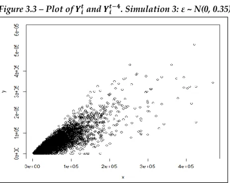
3.1.1 - Aim of the simulation ... 71
3.1.2 - Main simulation steps ... 73
3.1.3 - Simulation results ... 74
3.2 - Simulation in the case of stratified population ... 93
3.2.1 - Aim and main steps of the simulation study ... 93
3.2.2 - Results of the simulation ... 95
CHAPTER 4 Application to real data ... 99
4.1 - An application to the service turnover survey data ... 99
4.2 - Standard error using the Taylor series approximation and a comparison with the bootstrap method ... 101
4.3 - A comparison with the Knottnerus and Van Delden results about the standard error of the turnover growth rate in Dutch supermarkets ... 106
Conclusions ... 109
Appendix ... 113
Introduction
This work was inspired by the growing need to have a measure of the accuracy of the estimates produced within the short-term statistics in the Official Statistics. In particular, the aim of the work is to illustrate the methodology for the computation of the variance for the estimators currently used in the service turnover survey carried on by the Italian National Institute of Statistics (ISTAT) for the quarterly turnover growth rate estimation. The variance for the estimators currently used in the service turnover survey is computed only for the total estimations in the quarters t and t-4, while the variance of the growth rate estimation for the different estimation domains is not calculated. My methodological contribution is not only to suggest how to assess the variance of possible estimators of the turnover variation over time, but also to compare such estimators with respect to their variance to identify the best one.
While the adopted methodologies are fairly uniform within structural statistics on companies, this does not happen for short-term statistics, where the situation is quite heterogeneous. In fact, at European level, as indicated in the Short-Term Methodologies Handbook by Eurostat (see Eurostat, 2006), the choice of methodologies to be implemented is left to the various National Statistical Institutes. This heterogeneity appears both at the sampling plan level and at the estimation methods level.
Short-term statistics measure the evolution of a phenomenon over time. Often, we are not interested in the value itself of the variables of interest, but rather in their variation over time. Changes can be measured as the difference between two quantities at different waves (for example the difference in unemployment rate between two consecutive quarters) or as the relative percentage difference between two quantities over time (e.g. the percentage change of turnover with respect to previous quarter or same quarter of the previous year). In these cases, the variance is important for the production of a confidence interval of the variation. Confidence intervals are useful not only to evaluate the reliability of the estimate, but also to understand if a variation is statistically significant. In fact, if the confidence interval does not contain the zero value, it means that the calculated variation is statistically different from zero.
While the calculation of the variance of the estimates produced for a given instant of time is now a good practice (also through the development of software packages), the same does not happen for the variation of two quantities over time. An estimator of variance must take into account of both the estimator and the sampling design (Wolter, K.M. (1985)). The biggest difficulty is that for many surveys, the samples for producing estimates in two different time are not independent each other, due to the rotation operations of the sample. In particular for business surveys, in order to take into account the birth-mortality of units in the population and changes in stratification variables (such as size category and type of economic activity), the sample is updated, and a part of the units is replaced with others. Surveys, such as the Italian EU-SILC survey and the Italian Labour Force survey (LFS), include a rotated panel sample, resulting in partially overlapping samples between two occasions (Gazzelloni (2006), Ceccarelli et al. (2008)). This means that in calculating the estimate of the variance of change over time, we need not only the estimates of the variances of the cross-sectional estimates, but also the covariance terms between cross-sectional estimates. Moreover, many indicators are non-linear functions of linear estimators (e.g. simple ratio, difference of ratios), therefore, to calculate their variance a first-order Taylor approximation can be used. This is the case, for example, for the variance estimations of the LFS-based indicators’ annual net changes (Ceccarelli et al. (2017)). Alternatively, balanced repeated replication (BRR) can be used (Moretti et al. (2005)).
Currently, two estimators for the turnover growth rate estimation in the domain of services are used. The first is based on the variation computed on the overlapping sample units in both occasions (the quarter t and the quarter t-4), while the second is based on the ratio of totals computed through calibration, using all observations in both quarters and not only the overlapping sample units (Bacchini et al. (2013), Chianella et al. (2013), Bacchini et al. (2014), Bacchini et al. (2015), Chianella et al. (2015)). Other two estimators are taken into consideration in this study. The first additional estimator is based on the ratio of totals computed through calibration using only the overlapping sample units in both occasions, while the second additional estimator is based on the ratio of the sample means calculated using turnover data on all respondent units over the two quarters. Therefore, four non-linear estimators are presented for the turnover growth rate: ratio of sample means at the periods t and t-4, and ratio of totals through calibration, both computed: (i) on all the respondents units at both occasions, and (ii) only on overlapping respondents units. The performance is assessed by a simulation study, which also
has the aim of exploring under which conditions it is better to use all the observations or only the overlapping observations. The change estimators and the corresponding estimators of the variance are defined at stratum and estimation domain level and take into account the use of a stratified sampling design and the updating of the sample due to a replacement of some units and to a dynamic stratification of the population.
This work is organized as follows.
The first Chapter provides an overview of the literature available about the variance of the change over time. Contributions of different authors are described, focusing the attention on different types of population (large/not large population; stratified/non-stratified population, with/without the hypothesis of no birth-mortality in the population).
Chapter 2 describes the methodology used in Istat for the quarterly turnover growth rate estimation in the service sector. The aim of this Chapter is to introduce the methodology for the computation of the standard errors for the quarterly turnover growth rate. The computation is performed using the Taylor series approximation, at stratum and estimation domain level. It is also provided the formula of the overlapping values over which the estimator using only the overlapping sample units between both occasions is better than the estimator using all observations in both occasions.
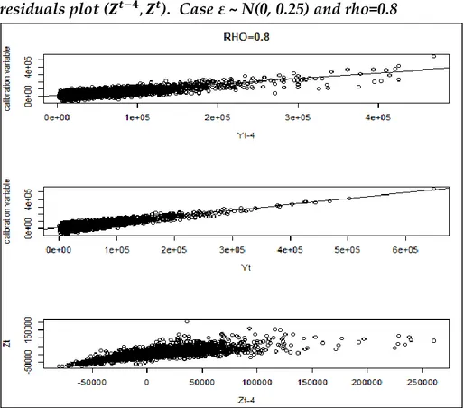
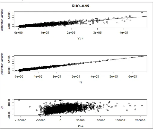
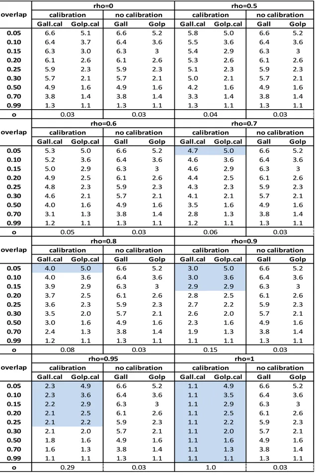
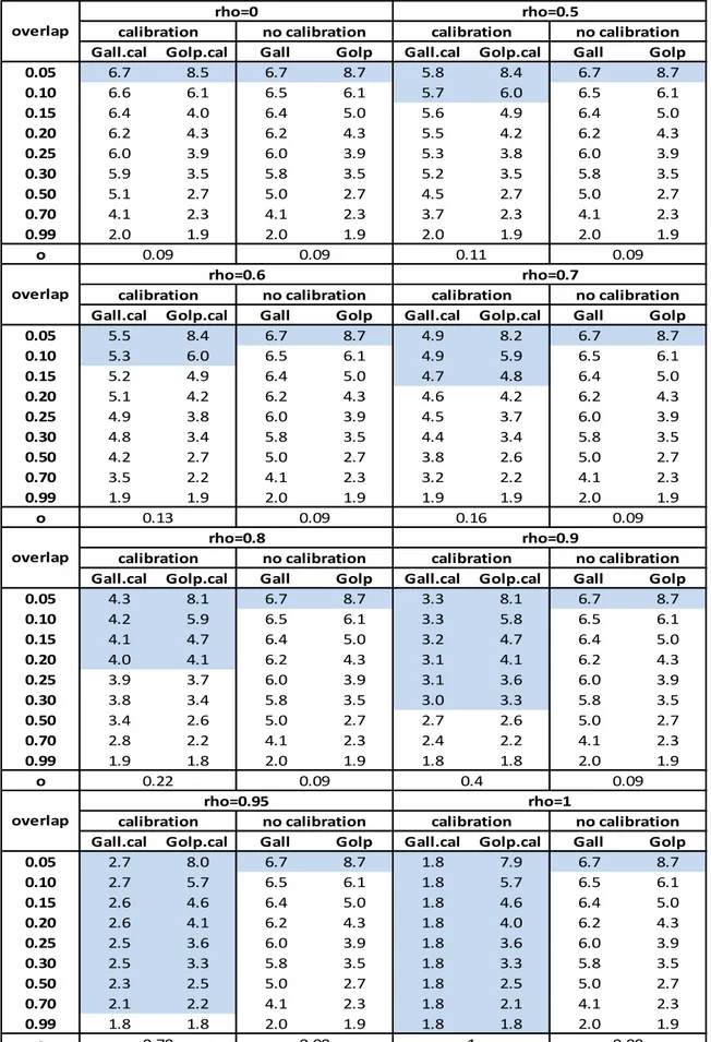
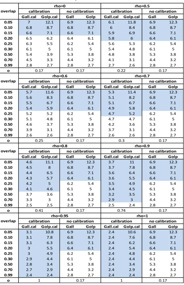
In Chapter 3, a simulation study was conducted with the aim of analyzing the performance of these estimators and exploring under which conditions it is better to use all the observations or only the overlapping observations. The bias, the standard deviation and the mean squared error have been analyzed through 1000 different samples extracted from the population, considering different values of the overlap between the respondent units at the occasions t and t-4 and different values of the correlation between the variable of interest and the calibration variable, together with different correlations between and . The estimator with minimum mean squared error was preferred.
In Chapter 4 an application performed on real data is described, using information from the quarterly service turnover survey with the aim to evaluate the standard errors associated with different estimates. A confidence interval is defined at 95% level. The standard errors obtained with the Taylor series approximation are compared with those obtained with the bootstrap method. The results are also
compared with the results obtained by Knottnerus and Van Delden (2012) about the standard error of the turnover growth rate in Dutch supermarkets.
CHAPTER 1
Literature on the variance of the change over
time
1.1 - The variance of change based on overlapping samples
from large populations
Suppose we are interested in estimating the change in the mean value in the population, of a quantity on two different occasions ̅ ̅. We use the difference between sample means calculated on two different occasions:
̂ ̅ ̅ .
The variance of the difference, can be expressed as:
( ̂) ( ̅ ) ( ̅ ) ( ̅ ̅ ) ( ̅ ) ( ̅ ) ( )
( ̅ ) ( ̅ ) ( )
where ∑ and ∑ .
Considering a simple random sample without replacement (srswor), with a fixed size of the sample , it is shown (Kish 1965, p. 63) that the variance and the covariance terms, are equal to:
( ) ( )
where and are the sample fraction and the sample size, respectively. In the general case, where we have two samples of different size, assuming that the population is the same over time (there is no birth-mortality), Kish (1965, pp. 457-466) obtains the general formula:
̂ ( ̂) ( ) ̂ ( ) ̂ ( ) ̂
( ) ̂ ( ) ̂ ( ) ̂
where ⁄ and is the size of the overlap units to both samples , (Figure 1.1). In the case of large population, the above expression becomes :
̂ ( ̂) ̂ ̂ ̂ ̂ ̂
̂ ̂
̂ ̂ ̂
̂ ̂ ̂ ̂ ̂
where the covariance term is written as the product between the correlation coefficient estimated from the common sample ̂ and the standard deviation ̂ ̂ , while the overlap in the first sample and in the second sample, are defined as:
Figure 1.1 - Two samples of different sizes ( and ) with overlap of size
Now, when ̂ ̂ ̂ and , the formula of the variance becomes: ̂ ( ̂) ̂ ̂ ̂ ̂ ̂ 𝑛𝑐 𝑛 𝑛 𝑠
̂ ̂ ̂ ̂
( ̂ ̂ )
If the correlation ̂ is positive, when we have complete overlap between the two sample at the different occasions ( ), then the variance of the difference ̂ will take its smallest value.
From the general case, Kish reports four particular cases, where the first two, concern the extreme cases of non overlap and complete overlap between the samples:
Case 1. There is no overlap between the two samples ( )
In this case (Figure 1.2), we have that and from the general formula of the variance of the difference, we obtain:
̂ ( ̂) ̂ ̂
Therefore in this case the covariance term does not attend to lower ̂ ( ̂)
Figure 1.2 - Non overlap between the sample
Case 2. There is complete overlap between the two samples ( ).
In this case (Figure 1.3), we have that . The formula of the variance becomes:
̂ ( ̂) ( ̂ ̂ ̂ ̂ ̂ )
𝑛
Figure 1.3 - Complete overlap between the sample
Case 3. The samples have identical size and partial overlap ( )
In this case (Figure 1.4), . The formula for the variance of the difference can be written:
̂ ( ̂) ̂ ̂ ̂ ̂ ̂
( ̂ ̂ ̂ ̂ ̂ )
Compared to case 2, we have now the term in the formulation. Since , ̂ ( ̂) will be higher with respect to the case of complete overlap between the samples.
Figure 1.4 - Samples with the same size and partial overlap
Case 4. The sample at the second occasion is a subset of the first
In this case (Figure 1.5), we have . It follows that and . The formula for the variance, becomes:
̂ ( ̂) ̂ ̂ ̂ ̂ ̂ ̂ ̂ ̂ ̂ ̂ 𝑛𝑐 𝑛 𝑛 𝑛𝑐 𝑛 𝑛
From this formulation can be noted that if ( ̂ ̂ ̂ ̂ ) , then more increase the size of the units not in overlapping (more is greater than ) and more increase the value of ̂ ( ̂).
Figure 1.5. The second sample is a subset of the first
1.2 - The variance of change without the hypothesis of large
population
The computation of the variance of ̂ becomes more complicated when the hypotesis of large population is removed. In fact, in finite populations, two disjoint samples are not independent.
Tam (1984) formulated the exact expression for the sampling variance of the difference ̂, removing the hypothesis of “large” population supposed in Kish. The finite population corrections now are not negligible. The general formula of a srswor in this case is:
̂ ( ̂) ( ) ̂ ( ) ̂ ( ) ̂
From the general formula Tam derived the formulas for three different sampling plans, assigning different values of f.
1. In the sampling plan A, at the first occasion we have a srswor of size from a population U. In the second occasion we have a sample consisting in the union of a random subset of the first sample ( , of fixed size ), and a srswor from U excluding the units in the first sample (see Figure 1.6). In this case and:
𝑛𝑐 𝑛
̂ ( ̂) ( ) ̂ ( ) ̂ (
) ̂
( ) ̂ ( ) ̂ ( ) ̂
If the size of the samples is the same in both occasions ( ), we can write:
̂ ( ̂) ( ) ( ̂ ̂ ) ( ) ̂
2. In the sampling plan B, at the first occasion we have a srswor of size from a population U. In the second occasion we have a sample consisting in the union of a random subset of the first sample ( , of fixed size ) and a srswor from U excluding the units in the overlap sample (see Figure 1.7). In this case
( )( ) ( ) and: ̂ ( ̂) ( ) ̂ ( ) ̂ ( ( )( ) ( ) ) ̂ ( ) ̂ ( ) ̂ ( ( )( ) ( ) ) ̂
3. In the sampling plan C, at the first occasion we have a srswor of size from a population U. In the second occasion the first sample is replaced with a srswor from U (see Figure 1.8). In this case is random and and:
̂ ( ̂) ( ) ̂ ( ) ̂
( ) ̂ ( ) ̂
As we can see in the above formulations, the smallest value of the variance of the difference between two cross sectional estimates, when there is overlap between samples, is obtained in the sampling plan B. This sampling plan is similar to that in the Italian survey for turnover (we will discuss on it in next chapters), with the
difference that at the second occasion the subset of the first sample is not completely random but there is a purposive choice.
Figure 1.6. Sampling plan A
Figure 1.7. Sampling plan B
Figure 1.8. Sampling plan C
Qualitè and Tillé (2008), also took into account two samples, and , selected without replacement and of fixed size and respectively. Then they considered , and , of random size (see Figure 1.9). The Horvitz-Thompson estimator is used for calculate the totals and and
𝑈 𝑈 𝑠 𝑠𝑐 𝑠 𝑠 𝑠𝑐 𝑠 𝑈 𝑈 𝑠𝑐 𝑠𝑐 𝑠 𝑠 𝑠𝑐 𝑠𝑐 𝑈 𝑈 𝑠 𝑠 𝑠𝑐 𝑠𝑐
considered the difference of totals ̂ . To compare the results with Tam we instead consider the difference ̂ ̅ ̅ .
Figure 1.9. Overlapping between two samples of fixed size of ,
Then we have:
( ̂) ( ̅ ) ( ̅ ) ( ̅ ̅ ) we can write:
( ̅ ̅ ) [ ( ̅ ̅ )] [ ( ̅ ) ̅ )]
Now, ̅ and ̅ are unbiased conditional on , thus:
[ ( ̅ ) ̅ )] ( ̅ ̅)
Furthermore, since we are in the sampling plan A of Tam, thus, as we show in the previous pages, the conditional covariance is:
( ̅ ̅ ) ( ) ̂ And hence: ( ̅ ̅ ) [( ) ] ( ( ) ) 𝑠𝐵 𝑠 𝑠 𝑠𝐶 𝑠𝐵 𝑠 𝑠 𝑠𝐶 𝑠𝐴
In this way the estimation of the variance of ̂ becomes:
̂ ( ̂) ( ) ̂ ( ) ̂ ( ( ) ) ̂ Where ̂ is the simple covariance, calculated from the sample :
̂
∑( ̅ )( ̅ ) A few comment on the above formula are in order.
1. If the two samples , form a panel we have that and we obtain:
̂ ( ̂) ( ) ̂ ( ) ̂ ( ( )
) ̂
( ) ( ̂ ̂ ̂ ).
2. If the two samples , , are disjoint ( ) then ( ) and:
̂ ( ̂) ( ) ̂ ( ) ̂ ̂
In this case, unlike the case 1 on Kish, conditionally on can lead the covariance term to increase the variance of the change ̂ (if the correlation between
and is positive).
Qualitè and Tillé also compare the variance of the estimator ̂ with the estimator ̂ ̅ ̅ , that considers the difference between the two cross sectional estimators only on the overlap between the samples. Also ̂ is unbiased conditional on .
Using the approximation ( )
( ) , the unconditional variance of ̂ is:
̂ ( ̂ ) [ ( ) ] ( ̂ ̂ ) [ ( )
( ) ( ) ] ̂ [ ( ) ] ( ̂ ̂ ̂ )
The difference ( ̂) ( ̂ ) is:
( ( ) ) ̂ ( ( ) ) ̂ ( ( ) ) ̂
( ( )) ̂ ( ( )) ̂ ( ( ) ( )) ̂
In the case , ̂ ̂ the authors obtained: ( ̂) ( ̂ ) (
( )) ̂ ( ( )
( )) ̂
Recalling that the overlap is (see the case 3 of Kish), in this case we can write:
( )
so that the difference of the variance between the two estimators becomes: ( ̂) ( ̂ ) [ ] ̂ [ ] ̂ ̂ ( )[ ( ) ] Therefore: 1) if ( ) : ( ̂) ( ̂ )
and the use of one estimator compared to the other one is indifferent 2) if
( ) : ( ̂) ( ̂ )
and the estimator that use only the overlap between the two sample ( ̂ ) is better than the estimator ̂
As we can see (Table 1.1), if the size of the overlap is considerable, then it is convenient to use the estimator ̂ , since a not too high value of the correlation is required.
Especially for economic surveys (e.g. the turnover survey), where the correlation between the observed variables over time is usually high, it is better to use the estimator based on the overlap ( ̂ ).
Table 1.1 When it is better to use the estimator ̂ for different overlapping rates overlap 0,1 >0,91 0,2 >0,83 0,3 >0,77 0,4 >0,71 0,5 >0,67 0,6 >0,63 0,7 >0,59 0,8 >0,56 0,9 >0,53 1 >0,50
1.3 - The variance of change in dynamic non-stratified
population
Laniel (1988) considered in his research, the case of the difference between levels in two consecutive occasion , removing the hypothesis of no birth-mortality in the population.
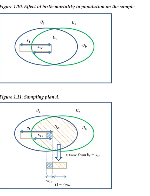
At the first occasion, Laniel considered a sample of size selected with srswor from the population . Between the first and second occasion there are change in the population, due to the birth-mortality of the units. At the second occasion, Laniel identified the units in the population that have survived from the first occasion ( ) and the new units ( ) referring to births. Laniel also identified the units in the sample that survived at the second occasion. We will refer to them with , of random size (Figure 1.10).
The sample at the second occasion comes from two independent sampling performed on and respectively.
He distinguished the sampling from in two cases, according to a modified version previously described in Tam.
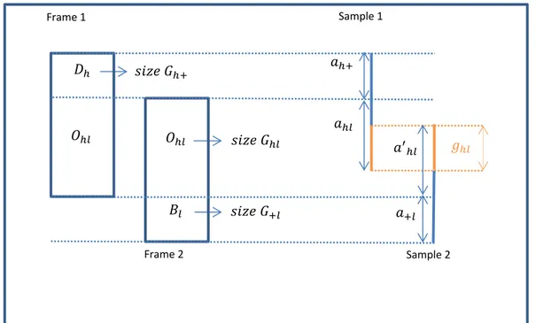
1. In the sampling plan A, a part of the first sample, of size (where ), is
randomly selected from the sample , while the remaining part, of size ( ) is
selected according to srswor from (see Figure 1.11).
2. In the sampling plan B, a part of the first sample, of size , is randomly selected
from the sample , while the remaining part, of size ( ) is selected
according to srswor from (see Figure 1.12).
Figure 1.10. Effect of birth-mortality in population on the sample
Figure 1.11. Sampling plan A
𝑠 𝑈𝑐 𝑈𝑏 𝑈 𝑈 𝑠 𝑐 𝑈𝑏 𝑈 𝑈 𝑈𝑐 𝑠 𝑐 𝑟𝑛 𝑐 ( 𝑟)𝑛 𝑐 𝑠 𝑠𝑟𝑠𝑤𝑜𝑟 𝑓𝑟𝑜𝑚 𝑈𝑐 𝑠 𝑐
Figure 1.12. Sampling plan B
The estimates for the total level in the two different occasions can be estimated through the expansion estimator.
At the first occasion, the estimate for the total is: ̂ ∑
At the second occasion, the estimate of , is given by the sum of the total in and the total in :
̂ ̂ ̂ ̂
∑
̂ ∑
where the expansion factor
is a random variable.
The formula of the variance of the difference between the two occasions is: ( ̂ ̂) ( ̂) ( ̂ ) ( ̂) ( ̂ ̂) 𝑈𝑏 𝑈 𝑈 𝑈𝑐 𝑠 𝑐 𝑟𝑛 𝑐 ( 𝑟)𝑛 𝑐 𝑠 𝑠𝑟𝑠𝑤𝑜𝑟 𝑓𝑟𝑜𝑚 𝑈𝑐 𝑟𝑠 𝑐
The variance for the total ̂ and ̂ , are known to be (Cochran, 1977, p.23):
( ̂) ( ) ( )
( ̂) ( ) ( )
Using Lemma 1 of Tam (1984, p.288), Laniel found the formula of the variance for ̂
( ̂) ( [
] )
where, following Sukhatme P. & Sukhatme B. (1970), and assuming sufficiently large,
[
] [ ( )( )
( ) ]
Using Lemma 2 and Lemma 3 of Tam (1984, p.289), Laniel found the estimate for the covariance between ̂ ̂:
( ̂ ̂)
{
( [ ])
( [ ] [
])
where in the above expression, supposing sufficiently large and using the second order Taylor’s formula, we have
[
]
( )( )
( )( )
Laniel found the formula of the estimate of the variance of the change between two consecutive occasions in dynamic population, but he did not consider that in many repeated surveys, in particular business surveys (eg. the italian quarterly service turnover survey), a stratified simple random sample without replacement (stratified srswor) is actually used.
1.4 - The variance of change in dynamic stratified
population
Tam (1984) and Qualité and Tillé (2008) do not provide an explicit form for stratification. However, under the assumption of a fixed population, fixed sample size and overlapping rate, and constant stratification over time, the result can be easily derived (Andersson, 2011):
̂ ( ̅ ̅ ) ∑ (
) ̂ ∑ (
) ̂
where ̂ is the covariance between and calculated on the common
sample within stratum .
Knottnerus and Van Delden (2012) considered in their research the case of rotating panels and population with dynamic strata and change in the population over time. In this case, there are three aspects that must be taken into consideration. 1. As specified in Holt & Skinner (1989) and Kitagawa (1955) in the case of a
stratified population, the net change in population means between two different occasions, ̅ ̅ , can be decomposed as a sum of a component referred to the change in population mean, assuming no change in the stratum composition in the population between the two occasions (A), and the change in the stratum composition (due to different stratum classification of the same units in both occasion or births and deaths), assuming no change in the mean within stratum (B):
̅ ̅
∑ ( ̅ ̅ ) ∑ ̅ ( )
In this formulation, as we can see, in the first term the stratum composition is fixed at the first occasion and we only measure the change in the mean within stratum while in the second term the mean within stratum is fixed at the first occasion and we measure only the change in the stratum composition between the two occasions.
2. Between two occasions, some units in the population could change their stratification variables value. This is very common for business surveys, where
one of the stratification variables can be the number of employees, so a different number of employees between one occasion and another can lead some units to be classified into different stratum over time. Because of these stratum migration, some estimates referred to a stratum “ ” on the first occasion, could be correlated with the estimates of the stratum “ ” on the second occasion.
3. As the population is repeatedly sampled, sample overlap may occur between the two occasions, as already discussed in the previous paragraphs.
Considering these aspects, Knottnerus and Van Delden derives the formula of variance for the yearly relative grow rate of Ducht monthly turnover in Supermaket. The survey is based on a rotating sample stratified by economic activity and size. The sample is monthly updated to take into account of births and deaths in the population. The sample is updated also in January of every year: the 10% of the sample is replaced with other units and the units that remain in the sample are stratified according to their actual size.
Due to the migration of units from one stratum to another, strata are probably composed by units with different inclusion probabilities. To solve this problem the authors form substrata that take into account the reallocation of the units from the stratum in December to the stratum in January. They define the following quantities
set of units in the population that have migrated from the stratum in december to the stratum in january, having size .
set of births in the population is the stratum , having size .
Let now ̂ be the relative change of the monthly turnover with respect to the same month of the previoulsy year:
̂ ̂
̂
and define further:
̂ ̂
̂ ̂
To estimate the variance of ̂ the authors use the first order Taylor expansion of a ratio between two estimators, obtaining:
( ̂ ) ( ̂ ) ( ̂ ̂ ) ( ̂ ̂ ) ( ) ( ̂ ) ( ) ( ̂ ) ( ̂ ̂ ) ( )
Considering the sampling design, the covariance term can be written as
( ̂ ̂ ) (∑ ̅ ∑ ̅ ) ∑ ∑ ( ̅ ̅ )
where ̅ and ̅ are the mean of the turnover in the sample in the stratum in month and in the stratum and in the same month of the previously year, respectively.
To take into account the reallocation of the units within stratum, and proceed with the analysis, the authors define the variables:
size of the units in the population that at the occasion t belong in the stratum while in the same month of the previously year belonged in the stratum ( ).
size of the units in the sample in the month ( )
within the substratum ( ): the size in can be different from that in because the units that belonged to and change stratum, can be not selected in t, thus no belong to
and ̅
are the total and the mean turnover, respectvely, within population
in month ( ), of the units that have migrated from the stratum to the stratum in january ( ).
and ̅
total and the mean turnover, respectvely, within the sample in
month ( ), of the units that have migrated from the stratum to the stratum in the population, between t-12 and t.
size of the overlapping units between the sample at the and occasion within the substratum .
̅ mean turnover in the month ( ) of the overlapping units, within the substratum
They define ( ) at the occasion t-12 and ( ) at the occasion t, to take into account the birth ( ) and the mortality ( ) respectively.
Then the ( ) term can be formuled as
( ̅ ̅ ) (∑ ̅ ∑ ̅ ) (∑ ̅ ∑ ̅ ) Since: ( ̅ ̅ ) for ( ̅ ̅ ) ( ̅ ̅ ) { ( ̅ ) ( ̅ )} { ( ̅ ) ( ̅ )} ( ̅ ̅ ) ̅ ̅ ( ) for we obtain: ( ̅ ̅ ) ( ̅ ̅ )
Conditionally on ( ), the covariance term can be expressed in
this way:
( ̅ ̅ )
( ̅ ̅ )
where the second term is equal to:
{ ( ̅ ) ( ̅ )} { ( ̅
) ( ̅ )}
̅ ̅ ( ) 1
Developing the first term and postponing the various steps to the paper of Knottnerus and Van Delden, we obtain
( ̅ ̅ ) { ( ) }
This expression can be estimated from the overlapping sample : ̂ ( ̅ ̅ ) ( ) ̂ where ̂ ∑ ( ̅ ) ( ̅ )
As is sufficiently large, this is a reasonable estimate while for small value could lead to a negative estimates in the numerator of ( ̂ ). For this reason, Knottnerus and Van Delden proposed an alternative estimator to ̂ , namely
̂ ̂ ̂ ̂ where: ̂ √ ∑ ( ̅ ) ( )
̂ is computed on the sample and is the estimate of the correlation
between and in .
With this estimator in the formula of the estimate of the covariance, they computed the confindence interval of the growth rates of the turnover for the ducht supermarket.
Summarizing the various steps, then we have:
1
Like described by the authors, we will see that Nordberg (2000) derived a different result for this expression
̂ ( ̂ ̂ ) ̂ (∑ ̅ ∑ ̅ ) ∑ ∑ ̂ ( ̅ ̅ ) ∑ ∑ ̂ ( ̅ ̅ ) ∑ ∑ ( ) ̂ ∑ ∑ ( ) ̂
Nordberg (2000), using inclusion indicators, derived the formula for the variance of change over time, considering dynamic stratified populations, with units that can migrate between strata. He calculated this formula for the business survey in Statistics Sweden. To increase the precision of the estimates overt time, the sampling design in Statistics Sweden is constructed by using the Samu system2.
This system is based on permanent random numbers associated with the units in the frame populations, and is used in particular to ensure a given overlapping between consecutive samples. A random number is associated with each units in the frame population at time 1 (frame1), then the frame is ordered by this number, and from a predeterminate starting point the first units within the stratum ( ( )) are selected. At time 2, there is a new updated frame population that take into account of birth-mortality on the enterprises (frame 2). Each unit in frame 2 that was also in the frame 1, maintains his permanent random number. At each new units a new random number is assigned, while units that were in frame 1 and no in the frame 2 are discarded. Then the units in the frame 2 are order on the basis of assigned random number, and from a starting point, the first units within the stratum ( ( )) are selected. To obtain the maximum overlap between the two samples, the starting point in frame 2 is the same used in frame 1. A random effect is due to the birth-mortality between the two populations over time.
2 See “Samu: the system for co-ordination of frame populations and sample from the Business Register at
Nordberg considers the estimates of the totals at time 1 and a time 2, obtained with both the Horvitz-Thompson estimator (H-T) and the Generalised Regression estimator (GREG). Then the estimates for the variable at time 1 ( ) and the variable at time 2 ( ) are functions of these totals. For istance, using the Horvitz Thompson estimator we obtain:
̂ ∑ ∑ ̂ ∑ ∑ where: { {
The estimates of and are then obtained as functions of totals ̂ and ̂
respectively:
̂ ( ̂ ̂ ̂ )
̂ ( ̂ ̂ ̂ )
The formula of the covariance in the expression of the variance of change ̂, can be written using a Taylor linearisation:
( ̂ ̂) ∑ ∑ ( ̂ ̂ ̂ ) ( ̂ ̂ ̂ ) ( ̂ ̂ )
where ⁄ , ⁄ and ( ̂ ̂) is the covariance between ̂ ̂ .
The units in the two populations can be split into death (D), overlapping (O) and born units (B).
Since the population is stratified, we can split the three groups D, O and B in ,
, , where:
is the subset of units belonging only to the frame 1, within stratum . Its size is
is the subset of the overlapping units between the two frame, within stratum
in frame 1, and in stratum in frame 2. Its size is .
is the subset of units belonging only to the frame 2, within stratum . Its size is
.
and are the size of the sample within stratum in the frame 1 and of the sample within stratum in the frame 2, respectively. They can be calculated as:
∑ ∑
where and are the size of the sample units belonging to the group and
respectively, while and are the size of the sample units at time 1 and at
time 2 respectively, belonging to the group . Furthermore, let be the size of
the sample overlapping units, belonging to the group . The rappresentation just
described is showed in Figure 1.13.
Nordberg use the random quantity { }
, to split ( ̂ ̂ ) in:
( ̂ ̂) ( ( ̂ ̂ )) ( ( ̂ ) ( ̂ ))
Figure 1.13. Frame population and sample units between the occasion 1 and 2
𝑎 𝑂 𝑙 Frame 2 Frame 1 𝐷 𝑂 𝑙 𝐵𝑙 𝑔 𝑙 𝑎 𝑙 𝑎 𝑙 Sample 1 Sample 2 𝑎 𝑙 𝑠𝑖𝑧𝑒 𝐺 𝑠𝑖𝑧𝑒 𝐺 𝑙 𝑠𝑖𝑧𝑒 𝐺 𝑙
Let's see now, how Nordberg calculates the two terms:
1) The covariance in the first term ( ( ̂ ̂ )), can be calculated as:
( ̂ ̂ ) ∑ ∑ ( ̂ ̂ ̂ ) ( ̂ ̂ ̂ ) ( ̂ ̂ )
Using the expression of the H-T estimators, we obtain:
( ̂ ̂ ) ∑ ∑ ∑ ∑ ( ) ∑ ∑ ∑ ∑ ( ( ) ( ) ( ))
The unbiased estimator for ( ̂ ̂ ) is:
̂( ̂ ̂ ) ∑ ∑ ∑ ∑ ( ( ) ( ) ( ) )
Nordberg also computed the first and second order inclusion probabilietis, and obtained: ̂( ̂ ̂ ) ∑ ∑ ̃ ( ̃ ) ( ̃ ) { ∑ ̃ ( ∑ ) ( ∑ )} where ̃ Hence: ̂( ̂ ̂ ) ∑ ∑ ( ̂ ̂ ̂ ) ( ̂ ̂ ̂ ) ̂( ̂ ̂ )
2) Nordberg considers the second term as a remainder term. He proposed a method to calculate it for the Swedish sampling disegn, trought a computer intensive
procedure with the Samu system. This term in Knottnerus and Val Deldend is instead estimated to be 0 (see again above). Nordberg estimates this term in this way: ( ( ̂ ) ( ̂ )) ∑ ∑ ( ̂ ̂ ̂ ) ( ̂ ̂ ̂ ) ( ( ̂ ) ( ̂ )) where: ( ̂ ) (∑ ∑ ( ) ) ∑ {( ∑ ) (∑ ∑ )} ∑ {( ∑ ) (∑ ∑ )} ∑ {( ̅ ) (∑ ̅ )} and similarly ( ̂ ) (∑ ∑ ( ) ) ∑ {( ∑ ) (∑ ∑ )} ∑ {( ̅ ) (∑ ̅ )}
Then, to estimate ( ( ̂ ) ( ̂ )) he applies the following procedure. He assigns a random number to each unit in the union of the two populations. Then such units are ordered by their random numbers, and the value is assigned to the firsts units within stratum of the first population, and the value is assigned to the firsts ordered units within stratum of the second population.
To the other units the valued is assigned. Then, the following quantities are computed: ( ) ∑ ( ) ( ) ∑ ( ) ( ) ∑ ( ) ( ) ∑ ( ) ̂ ( ) ∑ { ( ) ̅ (∑ ( ) ̅ )} ̂ ( ) ∑ {( ( ) ̅ ) (∑ ( ) ̅ )}
These values are calculated for . ̅ ̅ ̅ ̅ are the
sample means associated to ̅ ̅ ̅ ̅ . We can now calculate the
estimates for the covariance ( ( ̂ ) ( ̂ )), by:
̃ ∑ ( ̂ ( ) ̂ ( )) (∑ ̂ ( ))(∑ ̂ ( )) and then: ̂ ( ( ̂ ) ( ̂ )) ∑ ∑ ( ̂ ̂ ̂ ) ( ̂ ̂ ̂ ) ̃
1.5 - Other approaches
Berger (2004) also proposes a design-based estimator for covariance matrix that is adapted to overlapping samples between one wave and the next one, and he generalizes his results for stratified sample. He shows that his approach “yields non-negative definite estimates for covariance matrices and therefore positive variance estimates for a large class of measures of change”.
Berger, based his results on the aggregation of conditional covariances, using a Poisson sampling approximation of the actual sampling scheme. While Hajeck (1964) developed his approach for a single sample, Berger extends this approach to overlapping samples. His assumptions are “a fixed number of units rotating in
and out as well as a fixed number of units in the matched sample”. These assumptions “hold with most rotating sampling scheme”. However, as mentioned by Wood (2008) this method “involved a variety of matrix operations and no explicit covariance formula were presented”.
Osier & Raymond (2017) describe possible approach to estimates the variance for annual changes in the European Union Labour Force Survey (EU-LFS) based indicators. Almost all the countries of the European Union use a 2-(2)-2 rotating design: the units in the sample are interviewed for two consecutive quarters, then leave for two quarters and return in the sample for two more quarters of the following year. Therefore, they have to take into account the overlap between quarterly and annual data. They suggest to adopt an estimator proposed by Berger & Priam (2013) and Berger & Oguz Alper (2015). This estimator can be used with several EU-LFS sampling designs, and is easy to implement because it does not require the calculation of the joint inclusion probability, that can be unknown with rotating designs. It can be implemented by standard statistical software as R, SAS, SPSS, Stata, and requires minimal computing power. The idea is to estimate the design covariance matrix of ̂ and ̂ ( ̂) in:
̂ ( ̂) ̂ ( ̂ ) ̂ ( ̂ ) { ̂ ( ̂ ) ̂ ( ̂ )} ⁄ ̂ ̂
from the covariance of the residuals and of the following multivariate linear
regression model: ( ) ∑ ( ( ) ( ) ( ) ( ) ( ) ( ) ) ( )
where ( ) , and the residuals ( ) have a bivariate
distribution with null mean and unknown variance-covariance matrix. The covariate and are dummy design variables defined by:
{
{
The term, represents the interaction in the regression and take the rotation
of the design into account. The ( ) ( ) ( ) ( ) ( ) ( ) terms are the regression parameters of the model.
The model relies on the assumption that the sampling fractions are negligible, that is common thing for social survey like LFS. When we have large sampling fractions, which are common for example in business surveys, this approach is not suitable. Moreover, the estimator of the covariance matrix is unbiased only in the case of a large entropy.
One of the advantages of this approach is that the covariance matrix ̂ is
estimating using a single model, also if we have many stratum and totals. Moreover, in the case of the complex measures of the change ( ̂ ̂ ̂ or ̂
̂
̂ , where ̂ and ̂ are smooth functions of estimators of totals ̂ and ̂ ), using
Taylor linearization we have that:
̂ ( ̂) ( ̂) ̂ ̂( ) ( ̂)
where ( ) is the gradient of ( ) and the same estimated variance-covariance matrix ̂ can be used for several measures of change (any function of the same
totals). Therefore, the user, known the covariance matrix, have to define only the gradient. The estimate is possible without knowing the design and auxiliary variables because only the covariance matrix is necessary.
CHAPTER 2
Evaluation of the variance for the growth rate
estimators used in the Istat service turnover
survey
2.1 - Description of the survey and sampling design
The quarterly service turnover survey measures the quarterly percentage change recorded in sales at current prices by enterprises belonging to the domain of services (sections G, H, I, J, M, N of the Nace Rev. 2 classification), except for retail sales (G47). The indices are aggregated according to the Laspeyres formula, using a fixed weight structure that reflects the sectorial distribution of services turnover in the base year (figure 2.1). The quarterly service turnover index is obtained by aggregating all estimation domains.
The indicators produced up to March 2012 (G452, G46, H50, H51, H53, J) represented 60,1% of the total service turnover3. Istat’s strategic aim for the period
2010-2013 has been to complete the set of indices for the services sector as required by European Regulation (Regulation No 1158/05 of the European Parliament and of the Council, annex D). For the quarterly turnover indices, this implied the creation of new surveys to increase the coverage of the indices already produced for other economic activities.
The planning and launch of the new surveys allowed in March 2012 the dissemination of the indices for the sectors G45-G452, H49, H52, I55, I56, reaching 84,9% of the total service turnover and the completion of the indices for the G, H and I sections. Moreover, in 2013 the launch of new surveys related to M and N sections allowed to complete the total set of indicators required (for more details see Bacchini et al. 2015).
The turnover data are collected by a sample survey of about 17.000 enterprises. For the sectors where the market dynamics are determined by a small number of large companies (H50, H51, H53, J61, N78 domains of the Nace Rev. 2 classification), cut-off unit selection scheme have been adopted. In this case, the sample includes the biggest companies up to cover a sufficiently high share of the total turnover of the sector4 (usually over 80%).
Table 2.1- The weights structure in 2015 for the quarterly turnover indicators of services
Nace Rev. 2 Economic Activities Weights
2015
G45-G452 Wholesale & retail trade of motor vehicles and
wholesale & retail trade and repair of motorcycles 8.792
G452 Maintenance and repair of motor vehicles 1.168
G46 Wholesale trade, except of motor vehicles and
motorcycles 46.292
H49 Land transport and transport via pipelines 5.735
H50 Water transport 1.049
H51 Air transport 0.911
H52 Warehousing and support activities for
transportation 4.752
H53 postal and courier activities 0.509
I 55 Accomodation 1.977
I 56 Food and beverage service activities 4.704
J Information and comunication 9.237
M69 Legal and accounting activities 2.853
M70.2 management consultancy activities 1.240
M71 Architectural and engineering anctivities; technical
testing and analysis 2.097
M73 Advertising and market research 1.112
M74 Other professional, scientific and technical activities 1.304
N78 Employment activities 0.771
N79 Travel agency, tour operator and other reservation
service and related activities 0.992
N80 Security and investigation activities 0.325
N81.2 Cleaning activities 1.150
N82 Office administrative, office support and other
business support activities 3.030
Total 100.000
4
However, for most sectors a stratified simple random sampling without replacement (stratified srswor) is used. The stratification variables are the economic activity and the size of the enterprise. Businesses above a given size threshold (usually 100 employees) are included in self-representative strata. For some sectors, a specific size threshold (usually of at least 2 employees) is applied in the sampling selection of companies.
Every year, the sample size is computed by means of the Bethel algorithms implemented in Mauss-R (see Barcaroli et al. 2010). This allows to minimize the sample size, given the maximum expected sampling errors on target estimates for each type of domain5. Estimation domains are the sub-populations at which level
you want to compute the estimates of the parameters of interest. The precision required for the estimates, indicates the degree of reliability that the estimates have to guarantee. It is expressed in terms of the coefficient of variation (ratio between the standard error of the estimate and the estimate itself), to be specified for each parameter and each type of domain. The planned coefficient of variation for each estimation domain is fixed at 3%. The estimation domains are usually the 2 or 3 digits of the Nace Rev. 2 classification.
The auxiliary variables necessary for the allocation are stratification variables, that are essential to define strata and study domains, and the variables correlated with the variables of interest, useful for the study of their variability. The auxiliary information for the planning of the design is contained in the Istat Statistic Register of Active Firms (ASIA). The Register consists of economic units that run an activity in industrial and commercial sectors, as well as services to businesses and families sector. It provides identifying information (name and address) and business specific information (economic activity, employee number, activity start and end date, annual turnover) of these units6. The Register is annually updated
through a process of integration of information from both administrative sources and statistical sources. Its regular maintenance guarantees the update of the complex of active economic units over time, ensuring an official data source, harmonized at European level, on the structure of the population of enterprises and on its demographic characteristics. The Register (also used for the calculation of the national accounts estimates) has a central role in the field of economic statistics: it identifies the reference population for the sampling plans and for the carryover to the universe of the main surveys on companies conducted by Istat.
5
See the “User and methodological manual” about Mauss-R
The latest available ASIA contains a delay of two years. This means that for the year 2019, the latest Asia contains information updated to 2017. For this reason, within the service turnover survey an integration with sample data is used. In particular, the annual turnover sample values obtained from the quarterly observations and the number of employees replace the values contained in Asia. Due to the high correlation with the quarterly turnover, the variable used to study of the variability of the variables of interest is the annual turnover.
The sample is updated to account for both a re-stratification of the units and a sample replacement of approximately 15%. The units in the sample are re-stratified according to their actual size and economic activity from Asia. Dead companies are discarded from the sample, together with the companies that have been in the sample for several years. New companies are randomly selected from the last Asia available excluding the units already in the sample (plan A of Tam), until the theoretical size provided by the Mauss-R software is reached within each stratum. In this way between two consecutive years we have two overlapping samples.
The situation just described is represented in Figure 2.1. As we can see, between one quarter (t) and the same quarters of the previous year (t-4) we have two different partially overlapping samples, and . The overlapping sample is
represented by .
The overlapping units ( ) in the samples and could belong to different
stratum, because the stratification variable values can change across the two consecutive years.
Figure 2.1. Overlapping sample between two consecutive years
𝑠 rotated units 𝒔𝟐 overlapping sample 𝑠 new units 𝒔𝟏𝟐 𝒔𝟏 𝒔𝟐 𝒔𝟐𝟑 𝒔𝟐 𝒔𝟑 𝑡 4 𝑡 time Sample 𝑠 𝑠
New companies entering in the sample ( ) are required to indicate the turnover data for both the current year (t) and the previous year (t-4). In this way, it is possible to have turnover data for both estimation quarters, even if the firm was not in the sample at the occasion t-4.
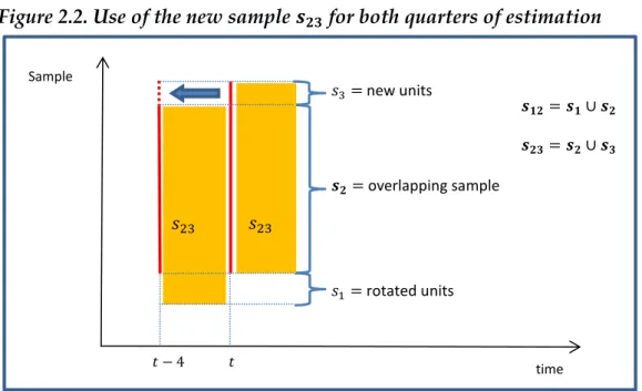
The estimates of the change between the occasion t and the occasion t-4 are both computed on the sample . It means that all observations are stratified in the
same way over the two estimation quarters, according to the latest information available on the stratification variables. The rotated units are not included in the estimates, neither in the quarter t nor in the quarter t-4.
The situation is shown in Figure 2.2. The dashed red line indicates data referred to the t-4 occasion that have been collected from the new enterprises entered in the sample at the occasion t ( ).
Figure 2.2. Use of the new sample for both quarters of estimation
2.2 - The methodology used for the growth rate estimation
As we have seen in the previous paragraph, the aim of the quarterly service turnover survey is the estimation of the percentage change of the turnover between the occasion t and t-4:
( ) ( ) 𝑠 rotated units 𝒔𝟐 overlapping sample 𝑠 new units 𝑡 4 𝑡 time Sample
Let be the set of the respondent enterprises only at the occasion t-4, the set of respondent enterprises on both occasions t-4 and t, the set of respondent enterprises only at the occasion t. Then we define and .
The completion of the indicators for all the service sectors represented an opportunity to review the estimation procedure for . For the new sectors, it is used a new estimation method that is different from the one used for the sectors already disseminated. In this section we analyze the two different methodologies.
2.2.1 - The estimator used for the sectors already disseminated
The estimation procedure for the sectors already disseminated before completing the indicator for all the service sectors is based on the variation computed on the overlapping sample units ( ) in both quarters. This means that only units in the sample that respond in both quarters are directly involved in the estimate. The
calculation of the change (G) is carried out at the stratum level. In formula, we can write: ̂ ̅̂ ̅̂ ∑ ∑ ̅̂ ̅̂
By applying ̂ to the index number of the same stratum of the previous year,
the stratum index for the current quarter is obtained: ̂ ̂
The elementary stratum index consists of two parts: the first one is the ratio between the two sampling averages of turnover at the current occasion and at the occasion t-4, calculated on the set of common respondents within the stratum h
( ̂ ). The second one is the published final stratum index for the same quarter
of the previous year. The second part takes into account the change in the average level of the turnover for the quarter t-4 compared to the same quarter of the base year. The index numbers are built in such a way that the average is equal to 100 in the base year.
The indices at the domain level are obtained by aggregating the stratum indices with an annual fixed weights system calculated via Asia, which takes into account the weights of the strata within the estimation domain, in terms of turnover:
̂ ∑ ̂
Finally, the turnover change at the domain level can be calculated as follows:
̂ ̂ ∑ ̂ ∑ ̂ ∑ ̅̂ ̅̂
2.2.2 - The estimator used for the new sectors
For the new sectors, instead, a methodology for the estimation of the totals in the population has been adopted, which is based on all respondent enterprises in the two occasions ( ). At the beginning the Horvitz-Thompson estimator has been computed and then a calibration estimator. Therefore, the initial sample weights are corrected using an auxiliary variable to account for non-response (Bacchini et al. 2014).
The change estimation at the stratum level through calibration is obtained by the ratio of the totals calculated within the stratum h:
̂ ̂ ̂ ∑ ∑
where and are the calibration weights associated with the j-th unit and i-th unit respectively. The calibrated weights ( and ) associated with the same unit on the two survey occasions of investigation (t and t-4) can be different due to the different non-response on the two occasions (the sets of respondent enterprises
and usually are not the same).
By summing up the totals of strata at the two occasions t and t-4, is possible to obtain the change estimation at the domain level:
̂ ∑ ̂ ∑ ̂ ∑ ∑ ∑ ∑
The calibration variable used is the annual turnover, due to its high correlation with the variable of interest. The values of the calibration variable and the known totals are the same in both the numerator and the denominator, and derive from the latest available Asia together with integration on sample data. Calibration is performed at single stratum level, i.e. the known totals are calculated for each stratum. The estimated totals for each stratum are aggregated within the estimation domains to allow the calculation of ̂ . By applying ̂ to the
index number of the same estimation domain for the previous year, the domain index for the current quarter is obtained as follows:
̂ ̂
The estimation methodology adopted for the new sectors has some advantages with respect to the one used for the sector already disseminated. It includes in the calculation of the index all respondent companies, and not only the overlapping observations, like in the estimator ̂ . In addition, the calibration can be
implemented using the software ReGenesees (R Evolved Generalized Software for Sampling Estimates and Errors in Surveys)7. This software is a full-fledged R
software for design-based and model-assisted analysis of complex sample surveys. This system is the outcome of a long-term research and development project aimed at defining a new Istat standard for calibration, estimation and sampling error assessment in large-scale sample surveys.
The advantage of using ReGenesees in the estimation process of the service turnover growth rate is that it provides the standard error related to the estimates of the totals (Chianella et al. 2013).
In 2013 different calibration models were tested (Bacchini et al. 2013). A comparison was made by integrating the annual turnover with other known information on the population. A list of different combinations of tested constraints is reported in the sequel. Annual turnover; annual turnover with employee number; annual turnover with company number; annual turnover with company and employee number. The analysis was conducted on a 3-year time interval (2010-2012). The range of the confidence intervals produced on the quarterly total estimates was evaluated together with the congruence at the
7