Optical surveying techniques for 3D reconstruction of submerged archaelogical artefacts

(1)

(2)

(3)

To Ida and my family

“It is not enough to take steps which may someday lead to a goal; each step must be itself a goal and a step likewise.”

(4)

This thesis is concerned with optical surveying techniques for 3D reconstruction in underwater environment. In particular, it focuses on 3D modelling of archaeological areas, lying both in shallow and deep water. Virtual representations of archaeological sites are required by researchers in order to enhance study and preservation methodologies and also to ease promotion and dissemination.

The presented work mainly follows two research lines.

First, it tackles the main problems arisen for standard 3D reconstruction algorithms and procedures when applied on submarine datasets. Multi-View mapping algorithm has been investigated and enhanced in order to achieve high accuracy reconstruction of two submerged villae, despite the challenging context of Baia Archaeological Park. Then, the textured and high detailed models can be employed for different purposes; in particular, some examples of virtual exploration, simulation for device design and for intervention planning and monitoring are shown. The second research line deals with the implementation of a Simultaneous Localization and Mapping (SLAM) algorithm for Unmanned Underwater Vehicles (UUVs). Some datasets acquired by an UUV equipped with typical navigation sensors and with a stereo-camera have been processed through the implemented Extended Kalman Filter (EKF), in order to perform sensor fusion and enhance both vehicle tracking and 3D scene reconstruction. Additionally, Augmented State Kalman Filter (ASKF) has been implemented in order to exploit optical data for loop closure detection in order to reduce drift error, typical of dead-reckoning navigation.

(5)

Il presente lavoro di tesi si occupa di tecniche di rilievo ottico per la ricostruzione 3D in ambiente subacqueo. In particolare, si concentra sulla modellazione 3D di aree archeologiche, site sia a basse che alte profondità. Le rappresentazioni virtuali dei siti archeologici sono uno strumento sempre più utile per i ricercatori, al fine di migliorare le metodologie di studio e conservazione o per facilitare la promozione e la fruizione.

Il presente lavoro segue principalmente due linee di ricerca.

In primo luogo, affronta i principali problemi posti dall’impiego di algoritmi e processi standard di ricostruzione 3D, quando applicati su dataset subacquei. Algoritmo di Multi-View mapping sono stati studiati e migliorati, ottenendo la ricostruzione accurata di due villae sommerse, nonostante il difficile contesto del Parco Archeologico di Baia. In seguito, i modelli texturizzati possono essere utilizzati per diversi scopi; in particolare, vengono riportati alcuni esempi di esplorazione virtuale e di simulazioni per la progettazione di dispositivi e per la pianificazione e il monitoraggio degli interventi. La seconda linea di ricerca affronta la realizzazione di un agoritmo di Simultaneous Localization and Mapping (SLAM) per veicoli sottomarini (UUVs). Alcuni dataset acquisiti da un UUV, equipaggiato con i tipici sensori di navigazione e con una stereo-camera, sono stati elaborati dal filtro di Kalman esteso (EKF) sviluppato, al fine di eseguire una sensor fusion e migliorare sia il tracking del veicolo sia la ricostruzione 3D della scena acquisita. Inoltre, è stato implementato un filtro di Kalman a sati aumentati (ASKF) in modo da poter sfruttare i dati ottici per il rilevamento di eventuali chiusure di loop, operazione che permette di ridurre l’errore di deriva, tipico delle applicazioni di navigazione stimata.

(6)

At the end of this experience, I realize what a great opportunity I've had here. The fact that I reached this point is due to the help and influence of many others.

First, I would like to thank my supervisor, Fabio, whose enthusiasm, understanding and positive attitude encouraged me through these years. In addition, I would like to acknowledge my appreciation for all of the opportunities and experiences he has given me. I am also very grateful to all the people in my Research Group, from all my collegues to Professors Muzzupappa and Rizzuti, who always have been more than coworkers.

I am also really grateful to ViCOROB as a whole for hosting me in a really edifying research period and for providing some datasets used in this thesis. In particular, I would like to thank Professor Rafael Garcia (Rafa) and Nuno for their unlimited help and willingness, not only in research field. I also thank Dr. Jordi Ferrer (Pio) who developed the code I moved from, and who kindly gave his support whenever needed, even if I have never met him.

An affectionate thought is for all the guys in the lab, coming from all over the world, who shared with me the work but, most of all, dinners and free time.

Additionally I thank the CoMAS project that entirely funded this work.

I thank all my friends and housemates for all the moments spent together and for both serious and trivial discussions about research and life.

I cannot finish without thanking my beloved family for all of the love and support they have given me through the years. I always miss you, even if sometimes it could not seem so…

Lastly, but definitely first, thank you to Ida, the most precious discovery that I could have possibly made during my PhD experience. Thank you for being a source of joy and sweetness in my life and for the support that you and your lovely family provided beyond words.

(7)

i

LIST OF FIGURES

Figure II-1 Pinhole camera model. ... 8

Figure II-2 Harris detector: a) flat region; b) edge; c) corner, example taken from [39] ... 15

Figure II-3 Comparison of detectors for test sequence, non-maxima suppression radius 10 pixels: (a) Harris, 271 keypoints. (b) Hessian, 300 keypoints. (c) Laplacian, 287 keypoints. (d) SIFT, 365 keypoints. (e) SURF, 396 keypoints. (f) Preprocessed image actually used for detection, image taken from [38]. ... 16

Figure II-4 Comparison of detectors for test sequence, non-maxima suppression radius 15 pixels, keypoints are displayed at the initial images: (a) Harris, 419 keypoints. (b) Hessian, 439 keypoints. (c) Laplacian, 429 keypoints. (d) SIFT, 509 keypoints. (e) SURF, 484 keypoints. (f) Preprocessed image actually used for detection, image taken from [38]. ... 16

Figure II-5 In this example, SIFT was used for the matching. About 1000 features have been matched in the couple of images and most of them seem to be correct. ... 19

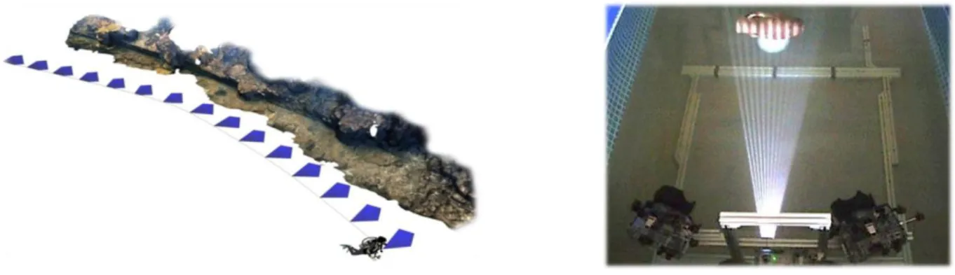
Figure II-6 Examples of acquisition by passive technique (left) and active technique (right). ... 21

Figure II-7 For every pixel m, the corresponding pixel in the second image m’ must lie somewhere along a line l’. This property is referred to as the epipolar constraint. See the text for details... 22

Figure II-8 Triangulation principle in active reconstruction. ... 24

Figure II-9 SFM reconstruction example. ... 25

Figure II-10 3D reconstruction sequence: point cloud, 3D virtual model (surface), 3D textured model ... 26

Figure II-11 Stereo triangulation example ... 27

Figure II-12Typical underwater imaging problem. Images taken from [112]. ... 32

Figure II-13 Shallow water light effects. Images taken from [113]and [114] ... 33

Figure II-14 Manned submersibles ... 35

Figure II-15 ROV ... 35

Figure II-16 AUV, Girona 500 ... 36

Figure II-17 LBL (a); SBL(b); USBL(c) and GIB systems (d). Images taken from [133] ... 38

Figure II-18 DVL sensors ... 41

Figure III-1 Geographical localization of Underwater Archaeological site of Baia (Italy). ... 48

Figure III-2 The Baianus Lacus. ... 49

Figure III-3 Underwater Archaeological Park: detail of Villa protiro ... 51

Figure III-4 Calibration panel used to manually correct the white balance. ... 52

Figure III-5 Image acquisition using a standard aerial photography layout (a) and oblique photographs (b). ... 53

Figure III-6 Original uncorrected image (a), acquired image using pre-measured white balance (b) and final corrected image (c). ... 54

Figure III-7 Sparse point cloud and 533 oriented frames. ... 55

(12)

vi

Figure III-9 Final textured 3D model (a). ... 58

Figure III-10 Final textured 3D model (b). ... 59

Figure III-11 Scheme of the three applications of 3D interactive environment. ... 60

Figure III-12: Screenshot of the application in realistic mode. ... 61

Figure III-13 Top: photo of Villa in Baia, bottom: screenshot of the application in realistic mode. ... 62

Figure III-14 Left: screen-shot of the application in study mode; right: top-view of study mode. ... 63

Figure III-15 Test of reachability for narrow edges and example of measuring. ... 63

Figure III-16 Underwater Archaeological Park: detail of Villa dei Pisoni ... 65

Figure III-17 3D surface and textured model of the site used to plan the cleaning intervention. ... 66

Figure III-18 The scale bar and a marker over the two areas selected to test the documentation process. ... 67

Figure III-19 3D reconstruction (with and without texture) of the uncleaned Area 1 and Area 2. ... 67

Figure III-20 Cleaning operations performed with nylon and stainless steel brushes. ... 68

Figure III-21 3D reconstruction (with and without texture) of the cleaned Area 1 and Area 2. ... 69

Figure III-22 Mesh deviations obtained comparing the cleaned and uncleaned surfaces. ... 70

Figure III-23 Cross-section analysis used to correlate the amount of removed material with the type of encrustation. ... 70

Figure V-1 Representation of world (in black) and local (in green) reference frames. ... 86

Figure V-2 Girona 500 equipment (left); Girona 500 AUV with its coordinate frame {v} and an example of a sensor frame {S} [211]. ... 86

Figure V-3 Left: Stereo matching. Right: temporal matching. ... 91

Figure V-4 Rectified quadruplet example and features matching: each vertex of triangulated structure represents a feature. ... 91

Figure V-5 Point 𝑀𝑖 is imaged at time 𝑡0 in the left and right camera of the stereo-rig at positions 𝑚𝑙0𝑖 and 𝑚𝑟0𝑖 respectively. Once the stereo-rig have moved the same world point 𝑀𝑖 is imaged in left and right camera coordinates 𝑚𝑙𝑖 and 𝑚𝑟𝑖. The stereo rig has a rigid transformation 𝑅𝑠, 𝑡𝑠 between left and right cameras. The estimated motion that the stereo-rig suffered is denoted by 𝑅, 𝑡 expressed with respect to the left camera frame. ... 95

Figure V-6 Plot of heading values. Considering intervals in which the observed parameter is supposed to be constant, it is possible to evaluate noise and, consequently, a good approximation for sensor covariance. ... 100

Figure V-7 EKF scheme ... 101

Figure V-8 Loop closure event ... 106

Figure V-9 La Lune. Left: the only known representation of the ’La Lune’ (first ship on the left), from a 1690 painting. (©Musée National de la Marine, S. Dondain, France).Right: bathymetry of the shipwreck (Girona) ... 109

Figure V-10 Left: Schema of the Girona 500 AUV, showing the location of principal components and payload area. Right: Deploying of the Girona 500 AUV above the La Lune shipwreck. ... 110 Figure V-11 Left: the whole trajectory surveyed by the AUV (two surveys have been performed on the

(13)

vii

Figure V-12 Sparse map estimated by Stereo-Tracker code with standard parameters. ... 111 Figure V-13 Sparse map estimated by Stereo-Tracker code with parameters adapted to maximize feature

matched. ... 112 Figure V-14 Left: Bathimetry of the area with sensor tracking elaborated by EKF in MATLAB (in red)

and by the AUV internal navigation EKF. Right: giga-mosaic of the area with pictures from longitudinal transect highlighted. ... 112 Figure V-15 Trajectory estimated by EKF for the left camera. ... 113 Figure V-16 Trajectory estimated by ASKF for the left camera: blue frames represent loop closures; red

frames are non-overlapping subsequent images. ... 114 Figure V-17 Loop closure detail ... 115 Figure V-18 Cap de Vol site in Agisoft Photoscan: 3D model(above) and camera poses resulting from

image registration (bottom). ... 116 Figure V-19 Top: La Lune trajectory estimated by C++ code (in blue) and by MATLAB EKF (in red)

based only on navigation sensors. Bottom: Cap De Vol trajectory estimated by C++ (in blue) and by Agisoft Photoscan bundle adjustment (in red). ... 118

(14)

viii

LIST OF TABLES

Table III-1 Results of the 3D reconstruction related to the cleaned and uncleaned areas ... 68

Table III-2 Results of the analysis conducted comparing the uncleaned and cleaned surfaces. ... 70

Table IV-1 Continuous-time Linear Kalman Filter [150] ... 75

Table IV-2 Discrete-Time Linear Kalman Filter [150] ... 78

Table IV-3 Discrete-Time Extended Kalman Filter [150] ... 80

Table V-1. Sensors employed in our underwater platform. ... 85

Table V-2 Generic 𝑃𝑖 matrix ... 104

(15)

1

I INTRODUCTION

Optical 3D reconstruction and mapping techniques have been widely investigated during the last few years. In particular, in the Cultural Heritage field, the use of digital models is becoming popular in application fields such as documentation, digital restoration, visualization, research and promotion [1, 2, 3]. Moreover, the increased Virtual Reality (VR) capabilities allow the employing of digitally modelled archaeological sites in order to promote their exploitation and facilitate the planning of conservation interventions.

This thesis, in particular, addresses the challenging problem of underwater 3D modelling. In effect, many underwater applications require gathering 3D data of flora, fauna, or submerged structures, for different tasks like monitoring, analysis, dissemination, or inspection. In particular, in the Cultural Heritage field, the reconstruction of submerged findings or entire archaeological sites is of great interest to researchers and enthusiasts, especially for inaccessible and hostile environments where data gathering is difficult and expensive. Moreover, according to the guidelines of UNESCO that suggest the in-situ preservation of underwater heritages [4], 3D reconstructions techniques and related tools have known a relevant growth in underwater archaeology field during the last decade. Among the various 3D techniques suitable for underwater applications, the photogrammetry represents a valid solution to reconstruct 3D scene from a set of images taken from different viewpoints. The data acquisition devices (both still and video cameras with the proper waterproof housings) are very affordable when compared to devices capable of providing range measurements such as LIDAR and multibeam echo sounders (MBES).Furthermore optical cameras can easily be deployed from underwater robots or handled by scuba divers to document the whole area of interest. When combined with specialized image processing techniques optical images allow the reconstruction of high-resolution textured 3D models.

The data gathering in traditional underwater archaeology is commonly performed via SCUBA diving but it is constrained by the practical depth that a diver can work (normally limited to 50 meters) and the time that can be spent underwater. New technologies, like manned submersibles or Unmanned Underwater Vehicles (UUVs) allow archaeologists to survey in very deep water while reducing operational costs. This increases dramatically the chance to acquire detailed morphometric data in underwater archaeological studies. Although technology plays a significant part in this work, it needs to be combined with the research methodologies used by archaeologists, so that archaeology in deep water conforms to the required standards [5]. Over

(16)

2

the last few years, it has been clearly demonstrated that archaeologists can benefit from new underwater technologies but their requirements pose new and sometimes fundamental problems for engineers [6], such as the need for very accurate navigation and high quality seabed mapping. Furthermore, imaging techniques in underwater suffer from particular problems induced by the medium, that have to be solved in order to achieve performances comparable with on-land activities, in terms of accuracy, resolution and acquisition time.

The combination of vehicle navigation and 3D mapping tasks is commonly known as Simultaneous Localisation And Mapping (SLAM). This is a well-known approach in robotics and it represents a very interesting tool for archaeological interventions and surveys and, in general, for any underwater robot operation. In effect, the possibility to accurately locate the underwater robot in a previously unknown scene can dramatically reduce the time and costs related to the data acquisition task. Previous works on terrestrial and aerial SLAM have produced impacting results [7, 8, 9], whereas in underwater environments there are still several issues to solve in order to achieve satisfying results. The main problem related to the subsea SLAM is that in the water the visible light and, in general, the electromagnetic waves suffer high attenuation and signal alterations. For this reason, different solutions have been investigated ranging from the use of acoustic devices (frequency-dependent range and resolution), near-field (1–5 m) vision, image enhancement and sensor fusion [10]. Thus, in this thesis two studies are presented: the former is intended to evaluate and optimize the performance of dense 3D mapping for documentation and monitoring purposes; the latter is addressed to improve underwater real-time SLAM by combining data from different sensors, usually employed in underwater navigation, with visual algorithms for pre-calibrated stereo-camera.

I.1 Context

The work of this thesis was developed within the framework of the CoMAS Project. CoMAS is an acronym for “COnservazione programmata, in-situ, dei Manufatti Archeologici Sommersi” (In-situ conservation of submerged archaeological artefacts) and its main aim is, indeed, the development of methodologies and tools oriented to the in-situ conservation of submerged archaeological artefacts. The most recent UNESCO guidelines for underwater cultural heritage prescribe the promotion, protection, and in-situ preservation (where possible) of underwater archaeological and historical heritage. This new orientation encounters a major difficulty related to the lack of knowledge, techniques, and materials suitable for underwater conservation because in the past

(17)

3

few decades, little attention have been devoted to subsea conservation studies, since the recovery of the findings had often been preferred. The CoMAS project is focused on the development of new materials, techniques, and methodologies for the conservation and restoration of subsea sites in their natural environment, according to criteria that is normally applied to the existing land Historic monuments.

In this context it clearly appears the need of carefully mapping the intervention scene; a map is a static and accurate representation of a space, mainly used to locate elements within them. Nowadays, 3D maps are a fundamental way to represent an area of interest and are widely used in a large amount of industrial and scientific application fields. In CoMAS, together with documentation, virtual restoration and exploration, 3D models of interested areas become essential for planning and monitoring the conservation activities of submerged remains and artefacts.

The CoMAS project includes the development of a Remotely Operated Vehicle (ROV) devoted to the routine cleaning and maintenance of the submerged sites. This specific task requires the accurate localization of the vehicle within the operation environment and a clear representation of the submerged scene in presence of low visibility conditions.

The case study for the CoMAS project is Baia of Bacoli (Naples, Italy). Its remarkable submerged Archaeological Park represents an ideal test scenario. In particular, it is a critical area because of the high level of turbidity, the heavy presence of marine flora, and the changing of lighting conditions, typical of shallow water, which can seriously affect the acquisition, thus compromising the reliability and the accuracy of the results.

Part of the work on underwater SLAM has been conducted in collaboration with the ViCOROB, a research group in Computer Vision and Robotics of the University of Girona, in Spain. In particular, the Underwater Vision Lab (UVL) team is a leader group in research and development of Unmanned Underwater Vehicles (UUVs) for accurate seafloor mapping and light intervention. For many years, they have dealt with different topics related to underwater vision and robotic for seabed analysis and reconstruction for different range of applications. Research interests encompass robot design and navigation, survey planning and simulation, 2D and 3D mapping of large areas with related underwater image processing requirements [11, 12, 13]. The ViCOROB knowledge in underwater application has gave a remarkable support to research activities related to underwater SLAM discussed in this thesis.

(18)

4

I.2 Motivation

Water covers more than 70% of our planet and, owning to hostile condition of deep seas, only a little percentage of seafloor is known and explored. The remaining part represents a potential huge source of information for biologists, geologists, archaeologists and many other researchers. Technology progress in recent times provide tools and methodologies to investigate this unknown world. UUVs can perform surveys in areas inaccessible to humans, and deploy a wide range of sensors useful for acquiring relevant data.

Maps are important tools to organize and store spatial information, and are of particular relevance as a display tool when that spatial information has a strong 3D content. Interest towards 3D mapping of the environment is considerably growing because of the possibilities provided by a detailed 3D model or map. Moreover, the latest progress in hardware and software performances allows achieving stunning results even with consumer cameras, so reducing related cost.

Virtual representation of objects and areas can be exploited both for study and dissemination aims. In addition, virtual visualisation and exploration in augmented reality can be very appealing tools.

Optical 3D imaging is even more promising for many disciplines related to the underwater field, because of the already discussed hostility of submarine environment.

The research topics investigated by the present work are ascribable to two very promising research lines:

 Dense 3D mapping with a single camera performed by scuba divers:

Scuba divers can perform acquisition of submerged scenes or objects lying at non-prohibitive deep by means of relatively low cost consumer camera. Taking care of underwater imaging peculiar aspects, it is possible to create impressive textured 3D model.

 Interactive 3D reconstruction for supporting ROV guidance and manipulation:

As in many applications, when operation scenario becomes hostile for humans, the better solution is to employ robotic platforms. In this case, due to depth and/or extent of interested scene, underwater vehicles become the only available option. In order to reduce risk and cost, UUVs are generally preferred to manned vehicles.

(19)

5

As mention above, the operation of UUVs faces important challenges related to their positioning inside the surveyed location. Consequently, it is necessary to have either a previously built map of the operation scene or to construct one during the surveying. Using optical sensing alone, it is extremely difficult to achieve the high standards for accurate positioning and map quality required by archaeologists. Among several factors, this difficulty is due to water turbidity, changes in natural light conditions in shallow water, and moving shadows when the robot it is fitted with artificial illumination in deeper water. For this reason, positioning data from other sensors will be exploited and used together with optical sensing.

I.3 Project Goals

Following the research lines highlighted in the previous section, the main goals of the presented work can be organised in two key topics. We try to explain briefly each of those, before giving an accurate analysis in the next Chapters.

 Experimentation of 3D dense mapping in complex underwater conditions.

Optical 3D reconstruction can be obtained in different manners and a series of previous studies available in literature or conducted in our Department tested different methodologies both in air and in water [14]. Among the most popular techniques, we tested the most affordable and promising ones to reconstruct some areas from the challenging context of Baia Archaeological Park. Chapter III points out how a certain care have been required during image acquisition and processing phases in order to optimise the results, and shows tangible contributions of accurate 3D mapping to planning and monitoring of conservation and restoration activities.

 Sensor fusion: Develop an EKF-ASKF for the interactive 3D mapping with UUV

Even in human reachable areas, UUVs employment can be useful to enhance operation performance surveying the interested area faster and more accurately than scuba divers do. Underwater visual SLAM, or simple 3D mapping, can take big advantages from sophisticate and accurate instrumentation equipping UUVs. It is possible to improve six-degrees-of-freedom (6DOF) tracking and 3D mapping from stereo pair capabilities, exploiting typical dead-reckoning navigation from sensors together with calibrated stereo-rig. A filter well known in navigation applications performs this sensor fusion: the Extended Kalman Filter (EKF), the non-linear counterpart of the Kalman Filter (KF). EKF is the de facto standard for navigation, able to give a

(20)

6

good estimate for different variables (the state vector) of a non-linear system, according to different sensor data and to the system model. In particular, we also implemented an Augmented State KF (ASKF), a modified version of the algorithm that stores and relate all state estimations in time, so providing trajectory optimization based on loop-closure detection. The final aim is to test the feasibility of a real time SLAM able to support ROV operator during intervention activities.

I.4 Thesis Structure

Thesis started with an overview of thesis main topics and objectives, presented in this Introduction Chapter. The work encompasses different topics (computer vision, underwater navigation and mapping, etc.).

Chapter II tries to gives an extensive background of all problems tackled in the thesis, of chosen approaches and relevant possible alternatives.

Then, Chapter III treats the 3D mapping for underwater archaeology; it briefly presents the CoMAS project, its motivation and its objectives, and the underwater Archaeological Park of Baia as selected case study. Two performed large area 3D reconstructions are shown, together with possible employment of the digital models in documentation, exploitation, intervention planning and monitoring over interested area.

Chapter IV discusses different Kalman Filter forms and gives detail on its theory and related formulae.

In Chapter V, we illustrate the implementation of an Augmented State Kalman Filter oriented to 6DOF SLAM for underwater vehicle navigation. The implemented filter gathers data coming from on-board navigation sensors and images from a stereo-rig; we analyse the Filter implementation procedure and its characterising models and assumption, referring both to MATLAB and C++ version.

Finally, a Conclusion Chapter summarizes topics and results and considers possible further developments and research lines.

(21)

7

II STATE OF ART

The state of art study is a fundamental step for any research activity. It is useful in order to know what has been already done in the interested field, to give new inputs, possible solutions and to support assumed hypothesis. Our research focuses about three main realms: underwater computer vision, underwater technology and their application in underwater archaeology. For the sake of simplicity, we tend to overlook or just briefly describe approaches, tools and methodologies not directly involved in the carried out research work.

II.1 A Review of Underwater Computer Vision

Computer vision is a widespread research field that covers diverse range of theory and application. Here, the discussion is focused on aspects related with image acquisition and their exploitation for 3D reconstruction, needed to the understanding of the work presented; we analyse principles of image formation and registration, mosaicking, 3D reconstruction techniques and we eventually show the main constraints peculiar to the marine environment.

II.1.1 Geometry of image formation

A digital image is a matrix of elements, the pixels (picture element), which contain the radiometric information that can be expressed by a continuous function. The radiometric content can be represented by black and white values, grey levels or RGB (Red, Green, and Blue) values.

Regardless of the method of acquisition of a digital image, it must be considered that an image of a natural scene is not an entity expressible with a closed analytical expression, and therefore it is necessary to search for a discrete function representing it.

The digitization process converts the continuous representation in a discrete representation, by sampling the pixels and quantizing the radiometric values. This is the process that directly occurs in a digital camera.

The imaging sensor collects the information carried by electromagnetic waves and measures the amount of incident light, which is subsequently converted in a proportional tension transformed by an Analogue to Digital converter (A/D) in a digital number.

The light starting from one or more light sources which reflects off one or more surfaces and passes through the camera’s lenses, reaches finally the imaging sensor. The photons arriving at this sensor are converted into the digital (R, G, B) values forming a digital image. In following

(22)

8

subsection, we discuss about some fundamental topics of image processing that deal with 3D reconstruction problem.

Pinhole Camera Model

The pinhole or perspective camera model (shown in Figure II-1) is commonly used to explain the geometry of image formation. Given a camera located at 𝐶 (the pinhole or the camera centre of projection) and an image plane placed at a distance 𝑓 (focal distance) from 𝐶, the pinhole model states that each light ray passes through 𝐶 and maps a generic point 𝑀 in 3D space to a 2D point 𝑚 lying on the image plane.

Figure II-1 Pinhole camera model.

With respect to the camera reference system {𝐶} we can refer to 𝑀 as 𝑀𝑐 (𝑋, 𝑌, 𝑍) and to 𝑚, its projection on image plane, as 𝑚𝑐 (𝑥, 𝑦, 𝑧). However, 3D points are often represented in a different coordinate system. Defining 𝑀𝑤 as the coordinates of 𝑀 in reference frame {𝑊}, it results that:

𝑴 𝒄 _{= 𝑹} 𝒘 𝒄 𝒘_𝑴_{+ 𝒕} 𝒘 𝒄 Eq. II-1

in which 𝑹𝒄 𝒘 represents a 3 × 3 rotation matrix and 𝒕𝒄 𝒘 represents a translation vector for 3D points. Writing the Eq. II-1 in matrix form, we obtain:

𝑀

𝑐 _{= [}𝑐𝑅𝑤 𝑐𝑡𝑤

(23)

9

where 𝑻𝒄 𝒘is the transformation matrix that represents the pose of the world reference frame with respect to the camera one.

Due to triangle similitude, and to the fact that 𝑧 = 𝑓 on image plane, 𝑐𝑀(𝑋, 𝑌, 𝑍) and 𝑚

𝑐 _{(𝑥, 𝑦, 𝑧) are related through the following:}

𝑥 = 𝑓 ∙𝑋

𝑍; 𝑦 = 𝑓 ∙ 𝑌 𝑍

Using homogeneous coordinates for 𝑚, this can be written in matrix form:

[ 𝑥 𝑦 1] = [ 𝑓 0 0 0 0 𝑓 0 0 0 0 1 0 ] [ 𝑋 𝑌 𝑍 1 ] Eq. II-3

The line through 𝐶, perpendicular to the image plane is called optical axis and it meets the image plane at the principal point.

Since the image coordinate system is typically not centred at the principal point and the scaling along each image axes can vary, the coordinates 𝑢, 𝑣 in frame {𝑖} undergoes a similarity transformation, represented by:

𝑻_𝒄

𝒊 _{= [}𝑠₀𝑥 _𝑠𝑠𝑠 𝑝𝑥 𝑦 𝑝𝑦

0 0 1] ; Eq. II-4

In which, 𝑠𝑥 and 𝑠𝑦 represent the relationship between pixel and world metric units (𝑝𝑥𝑠⁄𝑚𝑚) respectively along 𝑥 and 𝑦 axes (so giving the possibility to consider rectangular pixels); 𝑠_𝑠 is the skew coefficient related to the skew angle between frame vectors 𝑥 and 𝑦 (it differs from zero only if frame vectors are not orthogonal), and (𝑝𝑥, 𝑝𝑦) are coordinate of the principal point, expressed in image reference frame {𝑖}.

Adding this term to the perspective projection equation, we obtain:

[ 𝑢 𝑣 1] = 𝑻𝒄 𝒊 _[𝑓 0 0 0_{0 𝑓 0 0} 0 0 1 0 ] 𝑻𝒄 𝒘 𝒘𝑴 Eq. II-5 Alternatively, simply: 𝑚 𝑖 _{= 𝑷 𝑀}𝑤 _{Eq. II-6}

(24)

10

where 𝑷 is a 3 × 4 non-singular matrix called the camera projection matrix. This matrix 𝑷 can be decomposed as shown in Eq. II-7, where 𝑲 is the matrix containing the camera intrinsic

parameters, whereas 𝑹 and 𝒕 together represents the camera extrinsic parameters, namely the

relative pose of the world frame with respect to the camera.

𝑷 = 𝑲[𝑹|𝒕] 𝑤ℎ𝑒𝑟𝑒 𝑲 = [ 𝑓 𝑠_𝑥 𝑓 𝑠_𝑠 𝑝_𝑥 0 𝑓 𝑠𝑦 𝑝𝑦 0 0 1 ] Eq. II-7

The intrinsic parameters in 𝑲 can be parameterized by 𝑓, 𝑠𝑥, 𝑠𝑦, 𝑠𝑠, 𝑝𝑥 and 𝑝𝑦 shown in Eq. II-7. Thus, in the general case, a Euclidean perspective camera can be modelled in matrix form with six intrinsic and six extrinsic parameters (three for the rotation and three for the translation) which correspond to the six degrees of freedom for relative pose representation of world coordinate system with respect to the image coordinate system.

Nevertheless, real cameras deviate from the pinhole model due to various optical effects introduced by the lens system, visible as curvature in the projection of straight lines. Unless this distortion is taken into account, it becomes impossible to create highly accurate reconstructions. For example, panoramas created through image stitching constructed without taking radial distortion into account will often show evidence of blurring due to the misregistration of corresponding features before blending. Radial and tangential distortions are often corrected by warping the image with a non-linear transformation.

Following the distortion model presented in [15], we can consider the distorted image point 𝑚_𝑑 = (𝑥_𝑑, 𝑦_𝑑) in the real image can be related to its undistorted version 𝑚𝑢 = (𝑥𝑢, 𝑦𝑢) through radial and tangential terms, by means of the following equations:

[𝑥_𝑦𝑢 𝑢] = ( 1 + 𝑘𝑟1𝑟 2_{+ 𝑘} 𝑟2𝑟4+ 𝑘𝑟3𝑟6+ … ) [ 𝑥𝑑 𝑦𝑑] + 𝑑𝑡 where: 𝑑_𝑡 = [2 ∙ 𝑘𝑡1∙ 𝑥 ∙ 𝑦 + 𝑘𝑡2∙ ( 𝑟2+ 2 ∙ 𝑥𝑑2) 𝑘𝑡1( 𝑟2+ 2 ∙ 𝑦𝑑2) + 2 ∙ 𝑘𝑡2∙ 𝑥 ∙ 𝑦 ] ; 𝑟 2 _{= 𝑥}2_{+ 𝑦}2_;

Here 𝑘_{𝑟 ,}𝑘𝑡 .are radial and tangential distortion coefficients, and 𝑟 represents the distance of interested point from a hypothetic centre of distortion. Practically, tangential distortions are often less pronounced than radial ones and are ignored in some authors; common models consider up to the second or the third radial term and up to the second tangential one.

(25)

11

After evaluating the undistorted coordinates, we can map them to image plane through the intrinsic parameters, obtaining the pixel coordinates of associated point:

[ 𝑢 𝑣 1] = 𝑲 [ 𝑥𝑢 𝑦𝑢].

The explained problem of image formation onto image plane is just the reverse problem of interested one. We need, in effect, to recover the position in the 3D space of a point (or others visible elements) imaged at a certain pixel coordinates in the picture. This goal cannot be achieved from a single view of the scene. Analysing the Figure II-1 it clearly appear that each generic point 𝑀, belonging to the half line through 𝐶 and 𝑚 , gives the same projection 𝑚 on the image plane, so generating ambiguity that can be solved only by at least another view of the same point, as we later discuss.

Camera calibration

Intrinsic parameter evaluation is performed through a procedure known as camera calibration. In traditional camera calibration procedures, images of a calibration target represented by an object with a known geometry are first acquired. Then, the correspondences between 3D points on the target and their imaged pixels found in the images are recovered. The next step is represented by the solving of the camera-resectioning problem that involves the estimation of the intrinsic and extrinsic parameters of the camera by minimizing the reprojection error of the 3D points on the calibration object.

The camera calibration technique proposed by Tsai [16] requires a three-dimensional calibration object with known 3D coordinates, such as two or three orthogonal planes. This type of object was difficult to build, complicating the overall.

A more flexible method has been proposed by [17] and implemented in a toolbox by [18]. It is based on a planar calibration grid that can be freely moved jointly with the camera. The calibration object is represented by a simple checkerboard pattern that can be fixed on a planar board. It recovers required parameters using Direct Linear Transformation algorithm [19] and a non-linear optimization procedure.

This method can be very tedious when accurate calibration of for large multi-camera systems have to be performed; in effect, the checkerboard can only be seen by a small group of cameras at one time, so only a little part of camera network can be calibrated at the same time. Then it is necessary to merge the results from all calibration session in order to calibrate the whole camera set.

(26)

12

Svoboda et al [20] proposed a new method for multi-camera calibration, based on the use of a single-point calibration object represented by a bright led that is moved around the scene. This led is viewed by all the cameras and can be used to calibrate a large volume.

Although all these methods can produce accurate results, they require an offline pre-calibration stage that is often impractical in some application. Robust structures from motion methods, that allow the recovery of 3D structure from uncalibrated image sequences, have been developed thanks to the significant progress made in automatic feature detection and feature matching across images. Hence, the possibility to concurrently estimate both the camera trajectory and the camera projection matrix parameters (intrinsic and extrinsic values) is available in structure from motion algorithms used with videos [ 2 1 ] , or with large unordered image collections [22, 23]. Nevertheless, in order to reduce problem complexity and resource costs and also to increase model quality and robustness, a preliminary calibration step should always be carried out if possible.

II.1.2 Image Registration

Image registration is the process that aims to join two or more views of the same scene taken from different camera viewpoints but, more generally, also at different times or by different modalities (e.g. optical, infrared, acoustic, etc.).

In our case, as previously mentioned, image registration assumes great importance in order to reconstruct the 3D model of the scene reliably. Matching the same points in different images, in effect, can give information about object shape and also about camera motion in the scene; consequently, it is possible to recover, together with matched points, the relative pose of different views they are visible in, which is crucial information for 3D reconstruction that cannot always be available through other tools.

Image registration is a fundamental task for every activities involving more than one image. This task has application across many different disciplines spanning across scene change detection [24], multichannel image registration [25], image fusion [26], remote sensing [27], multispectral classification [28], environmental monitoring [29], image mosaicking [30], creating a super-resolution image [31], and as well aligning images from different modalities like in medical diagnosis [32].

(27)

13

Authors in [33] classify possible application in four main areas, according to the image acquisition setup:

 Different viewpoints (multiview analysis )

Images of the same scene are acquired from different viewpoints. The aim is to gain a larger 2D view or a 3D representation of the scanned scene [34].

 Different times (multitemporal analysis )

Images of the same scene are acquired at different times, often on regular basis, and possibly under different conditions. The aim is to find and evaluate changes in the scene, which appeared between the consecutive image acquisitions [35].

 Different sensors (multimodal analysis )

Images of the same scene are acquired by different sensors. The aim is to integrate the information obtained from different source streams to gain more complex and detailed scene representation [36].

 Scene to model registration

Images of a scene and a model of the scene are registered. The model can be a computer representation of the scene, for instance maps or digital elevation models (DEM) in GIS, another scene with similar content (another patient), “average” specimen, etc. The aim is to localize the acquired image in the scene/model and/or to compare them.

According to the Institute of Scientific Information (ISI), thousands of papers have been published during the last twenty years related to image registration, so confirming that it represent a crucial and on-going topic. Brown [37] did one of the most comprehensive surveys in 1992.

Due to the diversity of the images to be registered, and to various types of issues, it is impossible to design a universal method applicable to all registration tasks. Every method should take into account not only the assumed type of geometric deformation between the images but also radiometric deformations and noise corruption, registration accuracy and application-dependent data characteristics.

(28)

14

Nevertheless, the majority of the registration methods can be summarized in the following four steps:

 Feature Detection

Salient and distinctive objects (closed-boundary regions, edges, contours, line intersections, corners, etc.) are manually or (preferably) automatically detected. For further processing, these features can be represented by their point representatives (centres of gravity, line endings, distinctive points), which are called control points (CPs) in literature.

 Feature Matching

In this step, the correspondence between the features detected in the sensed image and those detected in the reference image is established. Various feature descriptors and similarity measures, along with spatial relationships among the features, are used for that purpose.

 Transform model estimation

The type and parameters of the so-called mapping functions, aligning the sensed image with the reference image, are estimated. The parameters of the mapping functions are computed by means of the established feature correspondence.

 Image resampling and transformation

The sensed image is transformed by means of the mapping functions. Image values in non-integer coordinates are computed by the appropriate interpolation technique.

Feature Detection

A very important requirement for a feature point is that it should be visually dominant and distinctive within the image. If it were not the case, it would not be possible to match it with a corresponding point in the other images. A traditional method for finding features is based on the measure of cornerness illustrated in Figure II-2. Some other detectors find blobs and ridges instead of corners. The main difference between the detectors is the manner to compute the cornerness

(29)

15

and the invariance of the detector to different geometry [38]. The main feature detectors are now summarized.

 Harris Corner Detection

The Harris corner methodology [39] underlies the idea of distinguishing the feature from the surrounding area image, because the neighbourhoods of the feature should be different from the neighbourhood obtained after a small displacement. By considering the difference between the patch centred on the pixel and the patches shifted by a small amount in different direction, the algorithm tests each pixel in the image to detect whether a corner is present or not. The Sum of the Square Difference SSD is computed by taking the sum of each pixel and its neighbourhood in one image and compare it with the SSD of all of the others pixels in the others images. The Harris corner technique is rotation invariant, invariant to linear changes in illumination, and robust to small amount of image noise.

Figure II-2 Harris detector: a) flat region; b) edge; c) corner, example taken from [39]

 Hessian Blob Detection

Beaudet was the first to develop this technique in 1978 [40]. He created an operator that is rotationally invariant given a determinant of the Hessian matrix.

The cornerness measured from Beaudet’s method is very good for blob and ridges detection. The region detected by the Beaudet method is nearly similar to the region detected by the Laplacian operator (see Figure II-3). It has been shown that the Hessian method is more stable than Harris method [41], even if it is less sensitive to the noise [42].

 Laplacian of Gaussian (LoG)

The Laplacian method is one of the most commonly method used blob detectors. This method is very robust for dark blob detection therefore very bad for bright blob detection [41].

(30)

16

Figure II-3 Comparison of detectors for test sequence, non-maxima suppression radius 10 pixels: (a) Harris, 271 keypoints. (b) Hessian, 300 keypoints. (c) Laplacian, 287 keypoints. (d) SIFT, 365 keypoints. (e) SURF, 396 keypoints. (f) Preprocessed image actually used for detection, image taken from [38].

Figure II-4 Comparison of detectors for test sequence, non-maxima suppression radius 15 pixels, keypoints are displayed at the initial images: (a) Harris, 419 keypoints. (b) Hessian, 439 keypoints. (c) Laplacian, 429 keypoints. (d) SIFT, 509 keypoints. (e) SURF, 484 keypoints. (f) Preprocessed image actually used for detection, image taken from [38].

 Scale Invariant Feature Transform (SIFT) Detector

The SIFT descriptor published by Lowe [43] uses the Difference of Gaussians (DoG), an approximation of LoG, to extract salient areas. The image 𝐼 is convolved with Gaussian kernels 𝐺 at different scales 𝑘, taking the difference 𝐷 between successive convolved images:

(31)

17

𝐷(𝑥, 𝑦, 𝜎) = 𝐿(𝑥, 𝑦, 𝑘𝑖𝜎) − 𝐿(𝑥, 𝑦, 𝑘𝑗𝜎);

𝐿(𝑥, 𝑦, 𝑘𝜎) = 𝐺(𝑥, 𝑦, 𝑘𝜎) ∗ 𝐼(𝑥, 𝑦); Eq. II-8 Convolved images are grouped by octave in which the 𝑘 parameter is doubled in subsequent levels of the image stack, called scale space. Local maxima and minima extracted from the this scale space represent the needed keypoints features, that are invariant with respect to image scaling, translation, rotation and partially invariant to illumination changes and affine or 3D projection. Furthermore, sub-pixel accuracy can be achieved using a quadratic Taylor expansion of the scale space.

 Speeded Up Robust Features (SURF) Detector

The SURF algorithm [41] is similar to SIFT in the scale space feature extraction using the determinant of the Hessian matrix.

𝐻(𝐼(𝑥, 𝑦, 𝜎)) = (𝐿𝑥𝑥(𝑥, 𝑦, 𝜎) 𝐿𝑥𝑦(𝑥, 𝑦, 𝜎)

𝐿𝑥𝑦(𝑥, 𝑦, 𝜎) 𝐿𝑦𝑦(𝑥, 𝑦, 𝜎)) ; Eq. II-9

In order to increase performances integral images are employed, together with box filters approximating Gaussian second order derivatives. It is possible, modifying the size of the filter, to have different responses thus obtaining the required scale space in which features are extracted.

 Maximally Stable Extremal Region (MSER) Detector

The MSER method developed by [44] is a blob detection algorithm. It uses a series of binarization, with threshold gradually increased, to extract zones with low variance over a large range of considered thresholds, corresponding to the higher or lower intensity values than all surrounding pixels.

Feature Description and Matching

For accurate image registration, features extracted from an image have to be correctly matched against the ones extracted from the other(s). Using statistics about just one pixel or small regions of pixels to characterize the feature would be highly instable in case of noise, illumination, and geometric changes. For these reasons, it is necessary to appropriately characterize the feature by choosing an adequate feature descriptor. State of art feature characterization methods are widely

(32)

18

discussed in [41, 45]. Here the discussion is focused on SIFT and SURF descriptors, that represent the most reliable ones. It has been shown that SIFT and SURF give better results in several applications and this makes them to be the most used descriptors [42]. Both approaches appears in hundreds of scientific publications because of their superiority with respect to correlation based methods, which can fail more frequently in underwater image registration. Different experiments in literature agree that SURF algorithm is very similar to SIFT in feature robustness, density, and reliability, but is significantly more performing in terms of the computational effort [41].

 SURF Descriptor

SURF descriptor is based on the distribution of intensity gradients around the features [41]. The use of gradients provides good feature distinctiveness. The SURF descriptor is extracted as followed:

In the first step, an orientation is obtained by calculating the wavelet response of Haar wavelets in 𝑥 and 𝑦 directions. The size of each Haar wavelet is four times the scale factor, and the size of circle around each point is six times the scale factor. The final orientation is achieved with reference to the total sum of wavelet responses within the sliding window. This sliding window covers an angle of 𝜋/3.

In the second step, in order to obtain the feature descriptor a square region is located at the central point with the reference to the selected orientation. This square is 20 times the scale factor and it is divided into 16 regions, each region is further divided into four smaller regions inside [38]. The final descriptor vector is based on the horizontal and vertical response of the Haar wavelet in each subregion; the descriptor is a four-element vector containing the absolute sum of horizontal and vertical responses of the Haar wavelet, this means that the final feature descriptor will have the length of 64 elements.

 SIFT Descriptor

The SIFT DoG detector gives invariance to translation and scale [43], and invariance with respect to rotation, change in illumination and 3D viewpoint can be managed by the descriptor. A local orientation is assigned to the detected keypoint as follows. The smoothed image 𝐿 is selected using the keypoint scale in such a way that all computations are performed in a scale-invariant manner. The keypoint’s scale can be different from all the ones represented in the scale space

(33)

19

levels. For each image sample, 𝐿(𝑥, 𝑦), at the closest scale the gradient magnitude 𝑚(𝑥, 𝑦) and the orientation 𝜃(𝑥, 𝑦), are obtained with pixel differences as:

𝑚(𝑥, 𝑦) = √(𝐿(𝑥 + 1, 𝑦 ) − 𝐿(𝑥 − 1, 𝑦 ))2 + (𝐿(𝑥, 𝑦 + 1) + 𝐿(𝑥, 𝑦 − 1))2 Eq. II-10

𝜃(𝑥, 𝑦) = 𝑎𝑡𝑎𝑛2(𝐿(𝑥, 𝑦 + 1) + 𝐿(𝑥, 𝑦 − 1), 𝐿(𝑥 + 1, 𝑦 ) − 𝐿(𝑥 − 1, 𝑦 )) Eq. II-11

Using the gradient orientations of points in the neighbourhood of the keypoint, an orientation histogram is obtained. Each point is weighted by its gradient magnitude using a Gaussian-weighted circular window with the standard deviation being 1.5 times the one of the keypoint scale. The highest peak in the histogram corresponds to the dominant direction of the local gradient and is detected, and other peaks within 80% of that value are used to create keypoints with that orientation. Only near 15% of points are assigned multiple orientations, but they increase the matching stability. A parabola is finally added to interpolate the peak position for better accuracy. The resulting SIFT keypoint comprises a vector (𝑥, 𝑦, 𝜎, 𝑚, 𝜃) with 𝑥, 𝑦 representing the coordinates, 𝜎 being the scale, and 𝑚, 𝜃 being the gradient magnitude and orientation, respectively. The SIFT descriptor can be also used with Harris, Hessian and Laplacian detectors. In these cases, the orientation is computed based on the keypoints detected by each detector in a single image, without considering scale invariance. The feature descriptors obtained by SIFT contain 128 elements, since the 4 × 4 descriptor array based on 8 bins orientation histogram was used. The set of keypoints given by the detection and the description process is used to find relations between two or more images. In general, depending on the images content and size, SIFT and SURF extract several hundred features, which are characterized by their spatial coordinates x and y, orientation θ, and scale.

Figure II-5In this example, SIFT was used for the matching. About 1000 features have been matched in the couple of images and most of them seem to be correct.

(34)

20

The basic criterion to associate features from two images is to find the nearest descriptors in terms of inner product between the descriptor vectors. In order to filter out associations between features with weakly discriminating descriptions (because they are too often present in the baseline, such as those that are extracted from background patterns often repeated), Lowe’s method [43] evaluates the nearest neighbour and second nearest neighbour of each descriptor. When the ratio of distances is smaller than 0.8, the match is rejected because it will be considered as ambiguous. By this criterion, Lowe managed to eliminate 90% of false matches, while losing less than five of correct matches, in the test data reported in [38].

II.1.3 Image mosaicking

Mosaicking is the task of combining two or more images such that the resulting composite image has an increased effective FOV. The problem has been extensively studied [46, 47, 48, 49, 50], with early roots in aerial and satellite imaging where the planar parametric motion-model is well approximated due to the large separation between camera and scene. Planar parametric motion-models yield a composite image that is theoretically exact under only two conditions [51]:

 the scene structure is arbitrary and the camera undergoes rotation about its optical centre

 the camera motion is arbitrary, but the scene being viewed is planar Both of these conditions are equivalent to no observed parallax in the input images.

Temporal Mosaicking

Early methods in mosaicking by the computer graphics community approached the problem in a temporally causal manner [46, 47, 48, 49, 50]. These approaches processed the imagery in a sequential manner to determine the pairwise homographies relating the temporal sequence, and constructed a composite view by concatenation (thus, warping all images to a common reference frame). While the pairwise homographies accurately describe the local registration, the small residual local alignment errors, coupled with errors in the applied motion-model, lead to an amplified global error when simply concatenated over long sequences. Since the image to reference frame homographies calculated by compounding do not attempt to achieve global consistency, images that are not temporal neighbours, but are spatial neighbours, may not be co-registered in the resulting mosaic.

(35)

21

Global Mosaicking

More recently, efforts have focused on imposing the available non-temporal spatial constraints to produce a globally consistent mosaic [52, 53, 54, 55]. These methods formulate the problem as the optimization of a global cost function parameterized by all of the image to mosaic frame homography parameters. The mosaic topology may initially be derived in a coarse manner assuming simplified motion-model parameters between temporally connected neighbours. From this roughly estimated topology, new spatial neighbours are hypothesized and then tested. This process is iterated until a stable image topology emerges. The optimization of the cost function incorporates these spatial constraints to produce a globally consistent mosaic with enhanced quality and robustness as compared to simpler mosaicking methods.

II.1.4 3D Reconstruction Techniques

During last few decades 3D reconstruction techniques have been widely investigated and improved. Our study focused on reconstruction techniques commonly employed, moving on from different reviews available in literature [56, 57, 58, 59] and from previous works conducted by our Department [14].

Optical reconstruction techniques allow obtaining a 3D digital model of real objects using pictures or videos of it. Image-based 3D modelling techniques (also called imaging techniques) are usually classified into passive, if the lightning source, natural or artificial, is needed only to light the object, and active, if lightning source takes part in the 3D reconstruction process [60].

Figure II-6 Examples of acquisition by passive technique (left) and active technique (right).

Photogrammetric techniques have known an important development during the last decade. Comparison between passive and active techniques have been studied both in air [60] and in

(36)

22

water [61] and the influence of water on calibration procedures has been investigated, too [62, 63].

Hereafter, we only touch on active techniques whereas we analyses more deeply some peculiar topics of passive techniques that, according to many tests and authors, appear to be more practical and promising for underwater applications.

Epipolar Geometry

The epipolar geometry captures the geometric relation between two images of the same scene. When a 3D point 𝑀 projects to pixels 𝑚 and 𝑚′ onto two images, 𝑚 and 𝑚′ are said to be in correspondence. For every point in the first image, the corresponding point in the second image is constrained to lie along a specific line called the epipolar line.

Figure II-7 For every pixel m, the corresponding pixel in the second image m’ must lie somewhere along a line l’. This property is referred to as the epipolar constraint. See the text for details.

Every plane such as 𝜋 that contains the baseline (the line joining the two camera centres), must intersect the two image planes in corresponding epipolar lines, such as 𝑙 and 𝑙’, respectively. All epipolar lines within an image intersect at a special point called the epipole. Algebraically:

𝑚′𝑇_{𝑭 𝑚 = 0} _{Eq. II-12}

(37)

23

Points 𝑚 and 𝑚′ can be transferred to the corresponding epipolar lines in the other image, using the following relations.

𝒍 = 𝑭𝑻_𝑚′_𝒍′_{= 𝑭𝑚} _{Eq. II-13}

The epipoles are also the left and right null-vector of the fundamental matrix:

𝑭𝒆 = 0 𝑭𝑻_𝒆′ _{= 0} _{Eq. II-14}

Since 𝑭 is a 3 × 3 matrix unique up to scale, it can be linearly computed from 8 pair of corresponding points in the two views using Eq. II-12, which is often called the epipolar constraint. This is known as the 8-point algorithm. However, when the rank constraint is enforced, 𝑭 can be computed from seven pairs of correspondences, using the non-linear 7-point algorithm. Refer to [19] for the details. Any pair of cameras denoted by camera matrices 𝑷 and 𝑷′ results in a unique fundamental matrix. Given a fundamental matrix 𝑭, the camera pairs are determined up to a projective ambiguity.

Active and Passive Optical Techniques

3D active techniques involve the object illumination in the shape recover process. Particular kinds of artificial light sources illuminate the scene and are exploited to evaluate the position in space of image points. It is possible to achieve this aim through different ways, but all uses either time-delay or triangulation principles.

In particular, in the first category, relying on time delay, 3D reconstruction is based on the measurement of the time of flight (TOF) of a light pulse sent towards the object. Assuming a constant light speed, it is possible to calculate the distance from the device to the object.

Time delay active sensors are employed, instead, for large objects, i.e. architectures, rooms, walls and archaeological sites [64]. These sensors work on longer distances (i.e. 2 - 1000 m), but are less accurate than triangulation systems.

In the latter techniques, the geometry of the object is reconstructed thanks to the particular configuration of the measuring devices, which made possible the use of triangulation principles. The system has to be calibrated in order to know the extrinsic parameters and so the relative pose of source and sensor. In effect, looking at Figure II-8, being known the baseline 𝑑 (the distance