Annals of DAAAM for 2012 & Proceedings of the 23rd International DAAAM Symposium, Volume 23, No.1, ISSN 2304-1382 ISBN 978-3-901509-91-9, CDROM version, Ed. B. Katalinic, Published by DAAAM International, Vienna, Austria, EU, 2012 Make Harmony between Technology and Nature, and Your Mind will Fly Free as a Bird Annals & Proceedings of DAAAM International 2012
NEAR-MARKERLESS POSITION MEASUREMENT USING
GENETICS AND POINT-TRACING ALGORITHMS
PASINETTI, S[imone]
Abstract: this paper present the preliminary results of the development of a position measurement vision system. In particular the procedure for the point matching are reported. This is made with an algorithm divided into two different phases: the first one is for the initial maching, and uses special a genetic algorithm; the second one is for the measurement phase and uses the difference between different frame to compute the point matching. After the description of the algorithms there are the results and the discussion of some tests.At the end there are some coclusion that describe the next steps of the work.
Keywords: Vision system, genetic algorithm, poit-tracing algorithm
1.
INTRODUCTION
In the last decade masurement system based in machine vision have become widely accepted and used.
Such systems range from common commercial application such barcode reader to mechatronic solutions as a self-orienting robot, including a wide variety of uses outside the proper industrial field [1]. In fact machine vision is also found in public safety for buildings and traffic monitoring as well as in human motion capture [2].
For what concerns this latter field, the principal benefit of machine vision, which is its being contactless and with negligible loading effect, is counterbalanced by the expensive components involved, mainly the cameras but also single-use markers on the subject, and by the high setup and calibration time requied (high positioning accuracy).
A further limit of these systems is also found in the low flessibility of the setup, which usually has to be defined ex-ante for a specific given test.
A further limit of these systems is also found in the low flessibility of the setup, which usually has to be defined ex-ante for a specific given test.
This paper will present preliminar results of a vision system development aimed at reducing these disadvantages addressing in particular the high running costs and high setup time.
At this stage only results detailing the measurement procedure will be presented, assuming for calibration and feature extraction standard alghorithms which will retailored later on. In particular, the procedure for matching points detected by any number of different cameras will be detailed.
From each given n-tuple of camera pixel created in the proposed way, the relevant point position in space can be easily computed using a standard algorithm.
The proposed measurement algorithm is made up by two different phases: during the initial matching phase the coupling between points detected by the n cameras is performed thanks to a genetic algorithm, the following measurement phase instead matches markers tracking them using difference between frames.
A preliminary validation will also be presented using different case studies to test the method flexibility and its reliability in different conditions.
2.
METHODS
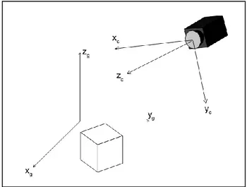
Below, there is a description of the two different phases of the point matching algorithm. The inputs of the first phases are the markers position related to the camera reference system {Xc, Yc, Zc}. The outputs of the whole
vision system are the position of the same markers related to the global reference system {Xg, Yg, Zg}
(figure 1).
Fig. 1. Reference system used.
To simplify the description of the algorithm the camera calibration phase and the feature extraction phase (to calculate the markers position related to the camera reference system using blob analysis [3]) are considered ultimated. They use typical procedure that you can find in the references ([4],[5],[6],[7],[8],[9], [10]).
The outputsof the algorithm are n-tuplas of coordinates (that represent the same marker referred to the coordinate system of each camera). The measure
-phase (after this algorithm) uses this n-tuplas to compute the markers position.
2.1 Genetic Algorithm
Genetics algorithms are a special optimization class of algorithms that use the concept of the reproduction mechanism used in nature.
In the references there are some papers that describe this kind of algorithms ([11],[12]).
This algorithms are based on the definition of a subject that is composed by genes with specific characteristics. This genes represent the parameters that the algorithm aims to minimize.
The first subject is called father_0 and represent the starting point of the algorithm.
After this definition, father_0 reproduces himself generating a number of children with the same genes of the father_0 but with different intrinsic characteristics (like that happen in nature). The children are similar but different to the father.
After the reproduction phase, the survive phase starts. An appropriate classification mechanism keep the children with better results and kills the others.
Only the survived children will be father in the next generation.
The survived children have genes that are better tha the other. With this procedure the genes intrinsic characteristic moves toward better values increasing the optimization each generation.
The algorithm ends when all the children born have the same gene characteristics, that means that the optimum subject is created.
In our system the inputs are represented by the markers position related to the camera reference system for each camera used.
If m is the number of the marker used and n is the number of the camera used at the beginning of the algorithm there are n matrix (2 x m dimension each one) that contains the coordinates of each marker (1).
𝑉𝑖= 𝑥𝑦11 𝑦𝑥22 𝑥𝑦33 ⋯ 𝑥⋯ 𝑦𝑚𝑚 𝑖 = 1 ⋯ 𝑛 (1)
Starting from this Vi matrices the initial subject (M)
will be made with the following characteristic:
Each column represent a single camera (n colums);
Each row represents a single marker (m rows);
Each element of the matrix M(i,j) is a number that represent the M-th marker of the Vi-th coordinates matrix defined above.
In this way the subjects contain only pointers to the the markers coordinates, giving more intuitive algorithm results.
The occlusion (that occurs when a camera can’t measure the position of some markers) are considered inserting a zero in the subject matrix placed in the
position related to the corresponding marker and the corresponding camera.
The algorithm can run only if each marker is seen by at least two camera. Without this hypothesis the 3D marker position can’t be found.
The markers coordinates are written in the Vi
matrices in a random order that depends by the recognition methods used.
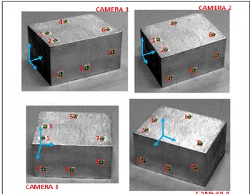
The father_0 is built according to the distance of the markers to the projection of the global reference system origin in the camera reference system. For example, for the figure 2, father_0 is represented by the matrix (2).
Fig. 1. Frame example for the creation of the initial subject (4 cameras, 7 markers) 1 2 3 4 5 7 6 1 2 3 4 5 6 7 1 3 2 4 5 7 6 3 2 4 1 5 7 6 (2)
After the creation of the first subject the algorithm proceed with the following phases:
1. father_0 reproduces himselves creating a fixed number of children. The reproduction is made in a probabilistic way: a certain percentage (92÷97%) of the genes of the father are reported to the child (that means that some genes stay in the same matrix row and column of the father), the remain genes are exchanged (they change the matrix row and column with other genes). With this technic each child is similar but not equal to the father.
2. Each child are then classified using the sum of the standard deviations calculated with the n-tupla of the marker coordinates (taken from Vi matrices) (3).
𝑇𝑒𝑠𝑡 = 𝑚𝑗 =1𝜎(𝑃𝑗) (3)
Pj are calculated using standard mesurement methods.
3. After the classification described above there is the survived phase: only the children with an high value of Test can be father in the next generation and the number of the children created from each one is directly proportional to the classification of the child. The children with a low value of Test die.
After this a new generation is created and the algorithm restarts from the point 2.
-In each generation the number of children remain constant to have always the same population size. This number can be modified by the user.In the chapter 3 some algorithm result are reported.
The genetics algorithm uses the first frame acquired from each camera to compute the initial markers matching. The second part of the algorithm starts using this matching, the frames acquired after the first and computing the difference between subsequent frames.
2.2 Point-tracing algorithm
After the analysis done on the first frame of each camera there is an initial matching of all the markers seen by the cameras.
From this point the second part of the algorithm starts. This phase use the difference between two subsequent frames of each camera to mantain the initial matching.
The point-tracing algorithm needs two basic hyppotesis:
High frame rate to have little difference between subsequent frame;
Camera synchronization to have frame synchronization.
To test this part only one camera was used, placed fixed in front of the tester avoiding the problems related to the camera synchronization (that occurs when more than one camera is used).
There are three kind of markers on the tester: red markers, blue markers and green marker. The algorithm works only on one color each step, thanks to a coloured filter placed before. In this way the distance of two markers increase and the probability of an uncorrect matching decrease. Using three different colour markers the measurement accuracy increase because it is due to the number of the markers used.
After the filter the algorithm starts: each marker of one frame is considered and it is related with all the markers in the subsequent frame. The distance between each couple of markers is computed.
There is a good matching when this distance is less than a fixed threshold T.
T is computed from equation (4) and depend to the distance between two near marker of the same colour (signed with D in the equation).
𝑇 =𝐷2 (4)
If the test give a negative response (no matching), that means that the marker of the first frame have no matching with all the markers of the subsequent frame.
If the marker has a positive test (matching ok), it will be discard for the next analysis to decrease the computational time comsumption.
3.
RESULTS
The two phases are then be tested in two different way.
For the first one (the genetic algorithm) the following parameters are used:
Population (number of children for each generation): 100;
Number of markers used: 5, 7, 13;
Percentage used in the reproduction phase (that represent the genes that change position in the subject): 2%, 3%, 5%, 8%, 30%.
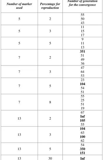
For each test you can see if the algorithm ends (finite number in “number of generation for the convergence” column), i.e. all the markers seen by the cameras are matched, and how many generation are needed for the convergence of the algorithm. Table 1 shows the results.
Number of marker used
Percentage for reproduction
Number of generation for the convergence
5 2 55 50 43 5 3 11 15 17 5 5 9 11 13 7 2 351 51 49 36 7 3 47 64 53 7 5 23 104 54 51 7 8 55 25 51 19 13 2 67 Inf 105 55 13 3 104 63 100 62 13 5 54 350 151 13 30 Inf
Tab. 1. Results of the convalidation of the genetics algorithm (the red number are the worse results)
In general when the reproduction percentage increase the number of generation needed to have the convergence of the algorithm decrease.
This happens only when few markers are used. In fact in the rows related to 13 markers an increasing of the reproduction percentage does not give a visible decrease of the number of generation for the convergence.
Furthermore, if the reproduction percentage became higher (till 30%) the number of generation became Inf and the algorithm diverge.
This happen because with an high probability for the markers substitution the children born from the father
-have many genes with different value from the father and the optimization does not happen.
A good value of this percentage that can be taken between 3% and 10%.
Seeing the first column is clear that an increase of the number of the markers used, increase the number of generation needed for the convergenve. This result seems to become stationary on 50-60 generation.
In some cases the algorithm diverge, i.e. there are some markers that are not matching between the cameras.
For the point-tracing algorithm only the bidimensional case are considered. In this test the number of the markers used is higher to increase the accuracy or the measure. There are three different coloured markers (red, blue, green).
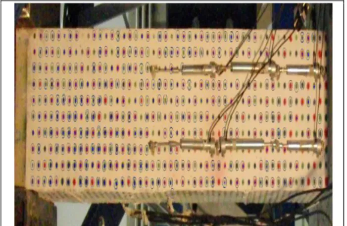
Figure 3 and figure 4 show the results. The pictures represent the overlapping of all the position measurements computed on all the frames acquired (in blue line). The background image is the first frame acquired.
Fig. 3. Result of the convalidation of the point-tracing algorithm. Strain test with 102 mm displacement
Fig. 4. Result of the convalidation of the point-tracing algorithm. Strain test with 3 mm displacement
The markers were drawn on a wall that is subject to a strain. The difference between the two test is the magnitude of the displacement: in the first one there are 102 mm displacement, in the second one there are 3 mm displacement.
The algorithm give a good matching result. In fact about all the markers are assigned correctly.
4.
CONCLUSION
In this paper there are the partial results of the development of a vision system for the position measurement. In particular the procedure for the matching of the point acquired by n-cameras are reported.
The system is composed by two different algorithms: the first one, used in the first measure phase, uses a genetic procedure for the first markers matching; the second one uses a method that compute the difference between subsequent acquired frames (point-tracing algorithm).
The tests shows that the first algorithm have a good result until the number of the markers used is low. A marker increasing, increase the number of the generation needed for the matchinf of all the markers. In some cases the algorithm diverge (not all the markers are matched).
The tests on the second algorithm show that this procedure give a good result, in fact, although the number of the markers used is high, a lot of there are matched. The tests are only for the bidimendional case (using only one camera).
The next steps of the work are the improvement of the genetic algorithm to have a good results with a large number of markers. In the next tests also the markers occlusions will be considered.
For the second algorithm the next step is the development of the tri-dimensional case.
For the two algorithms a decrease of the whole computational load is needed for the real time application. In fact now all the analysis are be done in post processing mode due to the high time comsumption needed.
5.
REFERENCES
[1] Beau, J. T,; Dah-jye, L.; James, K. A.; (2012). An on board vision
sensor system for small unmanned vehicle applications
[2] Thomas, B. M.; Erik, G.; (2000). A survey of computer
vision-based human motion capture
[3] Ming, A.; Ma, H.; (2007). A blob detector in color images [4] Mikolaijczyk, K.; Schmid, C.; (2005). A performance evaluation
of local descriptor
[5] Bay, H; Ess, A; Tuytelaars, T.; Van Gool, L.; (2007). Speeded-up
robust features (SURF)
[6] Derpanis, K. G.; (2007). Integral image-based rapresentations [7] Yonghong, X.; Qiang, J.; A new efficient ellipse detection method [8] Lowe, D. G.; (2004). Distinctive image features frome scale
invariant keypoints
[9] Lindeberg, T.; (1998). Edge detection and ridge detection with
automatic scale selection
[10] Cumani, A.; (1991). Edge detection in multispectral images