Search for supersymmetry with razor variables
in pp collisions at
p
ffiffis
¼ 7 TeV
S. Chatrchyan et al.* (CMS Collaboration)
(Received 15 May 2014; published 1 December 2014)
The razor approach to search for R–parity conserving supersymmetric particles is described in detail. Two analyses are considered: an inclusive search for new heavy particle pairs decaying to final states with at least two jets and missing transverse energy, and a dedicated search for final states with at least one jet originating from a bottom quark. For both the inclusive study and the study requiring a bottom-quark jet, the data are examined in exclusive final states corresponding to all-hadronic, single-lepton, and dilepton events. The study is based on the data set of proton-proton collisions atpffiffiffis¼ 7 TeV collected with the CMS detector at the LHC in 2011, corresponding to an integrated luminosity of 4.7 fb−1. The study consists of a shape analysis performed in the plane of two kinematic variables, denoted MRand R2, that correspond to the mass and transverse energy flow, respectively, of pair-produced, heavy, new-physics particles. The data are found to be compatible with the background model, defined by studying event simulations and data control samples. Exclusion limits for squark and gluino production are derived in the context of the constrained minimal supersymmetric standard model (CMSSM) and also for simplified-model spectra (SMS). Within the CMSSM parameter space considered, squark and gluino masses up to 1350 GeV are excluded at 95% confidence level, depending on the model parameters. For SMS scenarios, the direct production of pairs of top or bottom squarks is excluded for masses as high as 400 GeV.
DOI:10.1103/PhysRevD.90.112001 PACS numbers: 14.80.Ly, 12.60.Jv, 13.85.Rm
I. INTRODUCTION
Extensions of the standard model (SM) with softly broken supersymmetry (SUSY) [1–5] predict new funda-mental particles that are superpartners of the SM particles. Under the assumption of R-parity [6] conservation, searches for SUSY particles at the Fermilab Tevatron [7,8] and the CERN LHC [9–25] have focused on event signatures with energetic hadronic jets and leptons from the decays of pair-produced squarks ~q and gluinos ~g. Such events frequently have large missing transverse energy (Emiss
T ) resulting from the stable weakly interacting
super-partners, one of which is produced in each of the two decay chains.
In this paper, we present the detailed methodology of an inclusive search for SUSY based on the razor kinematic variables [26,27]. A summary of the results of this search, based on 4.7 fb−1 of pp collision data at
ffiffiffis p
¼ 7 TeV collected with the CMS detector at the LHC, can be found in Ref.[28]. The search is sensitive to the production of pairs of heavy particles, provided that the decays of these particles produce significant Emiss
T .
The jets in each event are cast into two disjoint sets, referred to as “megajets.”
The razor variables MR and R2, defined in Sec.II, are
calculated from the four-momenta of these megajets event by event, and the search is performed by determining the expected distributions of SM processes in the two-dimensional (MR, R2) razor plane. A critical feature of the
razor variables is that they are computed in the approximate center-of-mass frame of the produced superpartner candidates.
The megajets represent the visible part of the decay chain of pair-produced superpartners, each of which decays to one or more visible SM particles and one stable, weakly interacting lightest SUSY particle (LSP), here taken to be the lightest neutralino ~χ0
1. In this framework the reconstructed
products of the decay chain of each originally produced superpartner are collected into one megajet. Every topology can then be described kinematically by the simplest example of squark-antisquark production with the direct two-body squark decay ~q → q~χ0
1, denoted a “dijet plus EmissT ” final
state, to which the razor variables strictly apply.
The strategy and execution of the search is summarized as follows:
(1) Events with two reconstructed jets at the hardware-based first level trigger (L1) are processed by a dedicated set of algorithms in the high-level trigger (HLT). From the jets and leptons reconstructed at the HLT level, the razor variables MR and R2 are
calculated and their values are used to determine whether to retain the event for further off-line processing. A looser kinematic requirement is ap-plied for events with electrons or muons, due to the
* Full author list given at the end of the article.
Published by the American Physical Society under the terms of the Creative Commons Attribution 3.0 License. Further distri-bution of this work must maintain attridistri-bution to the author(s) and the published articles title, journal citation, and DOI.
smaller rate of SM background for these processes. The correspondence between the HLT and off-line reconstruction procedures allows events of interest to be selected more efficiently than is possible with an inclusive multipurpose trigger.
(2) In the off-line environment, leptons and jets are reconstructed, and a tagging algorithm is applied to identify those jets likely to have originated from a bottom-quark jet (b jet).
(3) The reconstructed objects in each event are com-bined into two megajets, which are used to calculate the variables MRand R2. Several baseline kinematic
requirements are applied to reduce the number of misreconstructed events and to ensure that only regions of the razor plane where the trigger is efficient are selected.
(4) Events are assigned to final-state “boxes” based on the presence or absence of a reconstructed lepton. This box partitioning scheme allows us to isolate individual SM background processes based on the final-state particle content and kinematic phase space; we are able to measure the yield and the distribution of events in the (MR, R2) razor plane for
different SM backgrounds. Events with at least one tagged b jet are considered in a parallel analysis focusing on a search for the superpartners of third-generation quarks. In total, we consider 12 mutually exclusive final-state boxes: dielectron events ELE), electron-muon events (ELE-MU), dimuon events (MU-(ELE-MU), single-electron events (ELE), single-muon events (MU), and events with no identified electron or muon (HAD), each inclusive or with a b-tagged jet.
(5) For each box we use the low (MR, R2) region of the
razor plane, where negligible signal contributions are expected, to determine the shape and normalization of the various background components. An analytic model constructed from these results is used to predict the SM background over the entire razor plane. (6) The data are compared with the prediction for the
background in the sensitive regions of the razor plane and the results are used to constrain the parameter space of SUSY models.
This paper is structured as follows. The definition of the razor variables is given in Sec.II. The trigger and off-line event selection are discussed in Sec. III. The features of the signal and background kinematic distributions are described in Sec.IV. In Sec.Vwe describe the sources of SM background, and in Sec.VIthe analytic model used to characterize this background in the signal regions. Systematic uncertainties are discussed in Sec. VII. The interpretation of the results is presented in Sec. VIII in terms of exclusion limits on squark and gluino production in the context both of the constrained minimal SUSY model (CMSSM)[29–31]and for some simplified model spectra (SMS) [32–36]. Section IX contains a summary. For the
CMSSM, exclusion limits are provided as a function of the universal scalar and fermion mass values at the unification scale, respectively denoted m0 and m1=2. For the SMS,
limits are provided in terms of the masses of the produced SUSY partner and the LSP.
II. THE RAZOR APPROACH
The razor kinematic variables are designed to be sensi-tive to processes involving the pair-production of two heavy particles, each decaying to an unseen particle plus jets. Such processes include SUSY particle production with various decay chains, the simplest example of which is the pair production of squarks, where each squark decays to a quark and the LSP, with the LSP assumed to be stable and weakly interacting. In processes with two or more unde-tected energetic final-state particles, it is not possible to fully reconstruct the event kinematics. Event by event, one cannot make precise assignments of the reconstructed final-state particles (leptons, jets, and undetected neutrinos and LSPs) to each of the original superpartners produced. For a given event, there is not enough information to determine the mass of the parent particles, the subprocess center-of-mass energypffiffiffisˆ, the center-of-mass frame of the colliding protons, or the rest frame of the decay of either parent particle. As a result, it is challenging to distinguish between SUSY signal events and SM background events with energetic neutrinos, even though the latter involve different topologies and mass scales. It is also challenging to identify events with instrumental sources of Emiss
T that can mimic the
signal topology.
The razor approach [26,27] addresses these challenges through a novel treatment of the event kinematics. The key points of this approach are listed below.
(i) The visible particles (leptons and jets) are used to define two megajets, each representing the visible part of a parent particle decay. The megajet reconstruction ignores details of the decay chains in favor of obtaining the best correspondence be-tween a signal event candidate and the presumption of a pair-produced heavy particle that undergoes two-body decay.
(ii) Lorentz-boosted reference frames are defined in terms of the megajets. These frames approximate, event by event, the center-of-mass frame of the signal subprocess and the rest frames of the decays of the parent particles. The kinematic quantities in these frames can be used to extract the relevant SUSY mass scales.
(iii) The razor variables, MR, MRT, and R≡ MRT=MR, are
computed from the megajet four-momenta and the Emiss
T in the event. The MRvariable is an estimate of an
overall mass scale, which in the limit of massless decay products equals the mass of the heavy parent particle. It contains both longitudinal and transverse information, and its distribution peaks at the true value
of the new-physics mass scale. The razor variable MR T
is defined entirely from transverse information: the transverse momenta (pT) of the megajets and the
Emiss
T . This variable has a kinematic end point at
the same underlying mass scale as the MRmean value.
The ratio R quantifies the flow of energy in the plane perpendicular to the beam and the partitioning of momentum between visible and invisible particles. (iv) The shapes of the distributions in the (MR, R2) plane
are described for the SM processes. Razor variable distributions exhibit peaks for most SM back-grounds, as a result of turn-on effects from trigger and selection thresholds as well as of the relevant heavy mass scales for SM processes, namely the top-quark mass and the W and Z boson masses. However, compared with signals involving heavier particles and new-physics sources of Emiss
T , the SM
distributions peak at smaller values of the razor variables. For values of the razor variables above the peaks, the SM background distributions (and also the signal distributions) exhibit exponentially falling behavior in the (MR, R2) plane. Hence, the
asymp-totic behavior of the razor variables is determined by a combination of the parton luminosities and the intrinsic sources of Emiss
T . The multijet background
from processes described by quantum chromody-namics (QCD), which contains the smallest level of intrinsic Emiss
T amongst the major sources of SM
background, has the steepest exponential falloff. Backgrounds with energetic neutrinos from W=Z boson and top-quark production exhibit a slower falloff and resemble each other closely in the asymptotic regime. Thus, razor signals are charac-terized by peaks in the (MR, R2) plane on top of
exponentially falling SM background distributions. Any SUSY search based on razor variables is then more similar to a “bump hunt,” e.g., a search for heavy resonances decaying to two jets[37], than to a traditional SUSY search. This justifies the use of a shape analysis, based on an analytic fit of the background, as described in Sec. VI.
A. Razor megajet reconstruction
The razor megajets are defined by dividing the recon-structed jets of each event into two partitions. Each partition contains at least one jet. The megajet four-momenta are defined as the sum of the four-momenta of the assigned jets. Of all the possible combinations, the one that mini-mizes the sum of the squared-invariant-mass values of the two megajets is selected. In simulated event samples, this megajet algorithm is found to be stable against variations in the jet definition and it provides an unbiased description of the visible part of the two decay chains in SUSY signal events. The inclusive nature of the megajets allows an estimate of the SM background in the razor plane.
Reconstructed leptons in the final state can be included as visible objects in the reconstruction of the megajets, or they can be treated as invisible, i.e., as though they are escaping weakly interacting particles[26]. For SM back-ground processes such as WðlνÞ þ jets, the former choice yields more transversely balanced megajets and lower values of R. If the leptons are treated as invisible in these processes, the Emiss
T corresponds to the entire W boson pT
value, similar to the case of Zðν¯νÞ þ jets events. B. Razor variables
To the extent that the reconstructed pair of megajets accurately reflects the visible portion of the underlying parent particle decays, the kinematics of the event are equivalent to that of the pair production of heavy squarks ~
q1, ~q2, with ~qi→ qiχ~01, where ~χ01denotes the LSP and qi
denotes the visible products of the decays as represented by the megajets.
The razor analysis approximates the unknown center-of-mass and parent particle rest frames with a razor frame defined unambiguously from measured quantities in the laboratory frame. Two observables MRand MRTestimate the
heavy mass scale MΔ. Consider the two visible four-momenta written in the rest frame of the respective parent particles: pq1 ¼ "m2 ~qþ m 2 q1− m 2 ~ χ0 1 2m~q ;MΔ 2 uˆq1 # ; pq2 ¼ "m2 ~ qþ m2q2− m 2 ~ χ0 1 2mq~ ; MΔ 2 uˆq2 # ;
where ˆuqi(i ¼ 1; 2) is a unit three-vector and mqirepresents
the mass corresponding to the megajet, e.g., the top-quark mass for ~t → t~χ0
1. Here we have parametrized the magnitude
of the three-momenta by the mass scale MΔ, where
M2 Δ≡ ½m2 ~ q− ðmqþ mχ~0 1Þ 2&½m2 ~ q− ðmq− mχ~0 1Þ 2& m2 ~ q : ð1Þ
In the limit of massless megajets we then have MΔ¼ ðm2
~ q− m2χ~0
1Þ=mq~
and the four-momenta reduce to
pq1 ¼ MΔ 2 ð1; ˆuq1Þ; pq2 ¼ MΔ 2 ð1; ˆuq2Þ:
The razor variable MR is defined in terms of the
momenta of the two megajets by
MR≡ ffiffiffiffiffiffiffiffiffiffiffiffiffiffiffiffiffiffiffiffiffiffiffiffiffiffiffiffiffiffiffiffiffiffiffiffiffiffiffiffiffiffiffiffiffiffiffiffiffiffiffiffiffiffiffiffiffiffiffiffi ðj~pq1j þ j~pq2jÞ 2− ðpq1 z þ pqz2Þ2 q ; ð2Þ
where ~pqiis the momentum of megajet qi(i ¼ 1; 2) and p qi z
is its component along the beam direction.
For massless megajets, MR is invariant under a
tudinal boost. It is always possible to perform a longi-tudinal boost to a razor frame where pq1
z þ pqz2 vanishes,
and MRbecomes just the scalar sum of the megajet
three-momenta added in quadrature. For heavy particle produc-tion near threshold, the three-momenta in this razor frame do not differ significantly from the three-momenta in the actual parent particle rest frames. Thus, for SUSY signal events, MR is an estimator of MΔ, and for simulated
samples we find that the distribution of MR indeed peaks
around the true value of MΔ. This definition of MR is
improved with respect to the one used in Ref.[26], to avoid configurations where the razor frame is unphysical.
The razor observable MR
T is defined as MR T≡ ffiffiffiffiffiffiffiffiffiffiffiffiffiffiffiffiffiffiffiffiffiffiffiffiffiffiffiffiffiffiffiffiffiffiffiffiffiffiffiffiffiffiffiffiffiffiffiffiffiffiffiffiffiffiffiffiffiffiffiffiffiffiffiffiffiffiffiffiffiffiffiffiffi Emiss T ðpqT1þ pqT2Þ − ~E miss T · ð~pqT1þ ~pqT2Þ 2 s ; ð3Þ where ~pT
qi is the transverse momentum of megajet qi
(i ¼ 1; 2) and pqi
T is the corresponding magnitude;
similarly, ~EmissT is the missing transverse momentum in
the event and Emiss
T its magnitude.
Given a global estimator MR and a transverse estimator
MR
T, the razor dimensionless ratio is defined as
R≡MRT
MR: ð4Þ
For signal events, MR
Thas a maximum value (a kinematic
end point) at MΔ, so R has a maximum value of approx-imately 1. Thus, together with the shape of MR peaking at
MΔ, this behavior is in stark contrast with, for example, QCD multijet background events, whose distributions in both MR and R2fall exponentially. These properties allow
us to identify a region of the two-dimensional (2D) razor space where the contributions of the SM background are reduced while those of signal events are enhanced.
C. SUSY and SM in the razor plane
The expected distributions of the main SM backgrounds in the razor plane, based on simulation, are shown in Fig.1,
[GeV] R M 0 500 1000 1500 2000 2 R 0 0.1 0.2 0.3 0.4 0.5 0 20 40 60 80 100 = 7 TeV s CMS simulation -1 L = 7.29 nb QCD(a) [GeV] R M 0 500 1000 1500 2000 2 R 0 0.1 0.2 0.3 0.4 0.5 0 1000 2000 3000 4000 5000 6000 7000 8000 = 7 TeV s CMS simulation -1 L = 4.7 fb W+jets, Z(νν)+jets(b) [GeV] R M 0 500 1000 1500 2000 2 R 0 0.1 0.2 0.3 0.4 0.5 0 500 1000 1500 2000 2500 = 7 TeV s CMS simulation -1 L = 4.7 fb tt(c) [GeV] R M 0 500 1000 1500 2000 2 R 0 0.1 0.2 0.3 0.4 0.5 0 1 2 3 4 5 = 7 TeV s CMS simulation -1 L = 4.7 fb SUSY LM6(d)
FIG. 1 (color online). Razor variables R2versus M
Rfor simulated events: (a) QCD multijet, (b) WðlνÞ þ jets and Zðν¯νÞ þ jets, (c) t¯t, and (d) SUSY benchmark model LM6[38], where the new-physics mass scale for LM6 is MΔ¼ 831 GeV. The yields are normalized to an integrated luminosity of∼4.7 fb−1except for the QCD multijet sample, where we use the luminosity of the generated sample. The bin size is 0.005 for R2 and 20 GeV for M
along with the results from the CMSSM low-mass bench-mark model LM6 [38], for which MΔ¼ 831 GeV. The peaking behavior of the signal events at MR≈ MΔ, and the
exponential falloff of the SM distributions with increasing MRand R2, are to be noted. For both signal and background
processes, events with small values of MR are suppressed
because of a requirement that there be at least two jets above a certain threshold in pT (Sec. III E).
In the context of SMS, we refer to the pair production of squark pairs ~q, ~q', followed by ~q → q~χ0
1, as “T2” scenarios [39], where the ~q' state is the charge conjugate of the ~q
state. Figure 2(a) shows a diagram for heavy-squark pair production. The distributions of MR and R2 for different
LSP masses are shown in Figs.2(b)and2(c). Figure2(d) shows the distribution of signal events in the razor plane. The colored bands running from top left to bottom right show the approximate SM background constant-yield contours. The associated numbers indicate the SM yield suppression relative to the reference line marked “1.” Based on these kinematic properties, a 2D analytical description of the SM processes in the (MR, R2) plane is developed.
III. DATA TAKING AND EVENT SELECTION A. The CMS apparatus
A hallmark of the CMS detector [40] is its super-conducting solenoid magnet, of 6 m internal diameter, providing a field of 3.8 T. The silicon pixel and strip tracker, the crystal electromagnetic calorimeter (ECAL), and the brass/scintillator hadron calorimeter (HCAL) are contained within the solenoid. Muons are detected in gas-ionization detectors embedded in the steel flux-return yoke, based on three different technologies: drift tubes, resistive plate chambers, and cathode strip chambers (CSCs). The ECAL has an energy resolution better than 0.5% above 100 GeV. The combination of the HCAL and ECAL provides jet energy measurements with a resolu-tionΔE=E ≈ 100%=pffiffiffiffiffiffiffiffiffiffiffiffiffiffiffiE=GeV⊕ 5%.
The CMS experiment uses a coordinate system with the origin located at the nominal collision point, the x axis pointing towards the center of the LHC ring, the y axis pointing up (perpendicular to the plane containing the LHC ring), and the z axis along the counterclockwise beam
[GeV] R M 500 1000 1500 2000 2500 a.u. 0 0.01 0.02 0.03 0.04 0.05 0.06 0.07 = 900 GeV χ = 1150 GeV, m q~ m = 750 GeV χ = 1150 GeV, m q~ m = 500 GeV χ = 1150 GeV, m q~ m = 50 GeV χ = 1150 GeV, m q~ m =7 TeV s CMS simulation (b) 2 R 0.1 0.2 0.3 0.4 0.5 0.6 0.7 0.8 0.9 1 a.u. 0 0.01 0.02 0.03 0.04 0.05 0.06 0.07 = 900 GeV χ = 1150 GeV, m q~ m = 750 GeV χ = 1150 GeV, m q~ m = 500 GeV χ = 1150 GeV, m q~ m = 50 GeV χ = 1150 GeV, m q~ m =7 TeV s CMS simulation (c) (a) [GeV] R M 500 1000 1500 2000 2500 2 R 0.2 0.4 0.6 0.8
1 3.0e-05 6.3e-08 1.2e-10 2.0e-13 3.3e-16
= 900 GeV χ = 1150 GeV, m q~ m = 750 GeV χ = 1150 GeV, m q~ m = 500 GeV χ = 1150 GeV, m q~ m = 50 GeV χ = 1150 GeV, m q~ m =7 TeV s CMS simulation (d)
FIG. 2 (color online). (a) The squark-antisquark production diagram for the T2 SUSY SMS reference model. The distribution of (b) MRand (c) R2for different LSP masses m~χin the T2 scenario. (d) Distribution of T2 events in the (MR, R2) plane for the different LSP masses m~χ. The orange bands represent contours of constant SM background. The relative suppression factors corresponding to some of the bands are indicated in the upper part of the figure.
direction. The azimuthal angle, ϕ, is measured with respect to the x axis in the ðx; yÞ plane, and the polar angle, θ, is defined with respect to the z axis. The pseudorapidity is η ¼ − ln½tanðθ=2Þ&.
For the data used in this analysis, the peak luminosity of the LHC increased from 1 × 1033 cm−2s−1 to over
4 × 1033 cm−2s−1. For the data collected between
ð1–2Þ × 1033 cm−2s−1, the increase was achieved by
increasing the number of bunches colliding in the machine, keeping the average number of interactions per crossing at about seven. For the rest of the data, the increase in the instantaneous luminosity was achieved by increasing the number and density of the protons in each bunch, leading to an increase in the average number of interactions per crossing from around 7 to around 17. The presence of multiple interactions per crossing was taken into account in the CMS Monte Carlo (MC) simulation by adding a random number of minimum bias events to the hard interactions, with the multiplicity distribution matching that in data.
B. Trigger selection
The CMS experiment uses a two-stage trigger system, with events flowing from the L1 trigger at a rate up to 100 kHz. These events are then processed by the HLT computer farm. The HLT software selects events for storage and off-line analysis at a rate of a few hundred Hz. The HLT algorithms consist of sequences of off-line-style reconstruction and filtering modules.
The 2010 CMS razor-based inclusive search for SUSY [26]used triggers based on the scalar sum of jet pT, HT, for
hadronic final states and single-lepton triggers for leptonic final states. Because of the higher peak luminosity of the LHC in 2011, the corresponding triggers for 2011 had higher thresholds. To preserve the high sensitivity of the razor analysis, CMS designed a suite of dedicated razor triggers, implemented in the spring of 2011. The total integrated luminosity collected with these triggers was 4.7 fb−1 atpffiffiffis¼ 7 TeV.
The razor triggers apply thresholds to the values of MR
and R driven by the allocated bandwidth. The algorithms used for the calculation of MR and R are based on
calorimetric objects. The reconstruction of these objects is fast enough to satisfy the stringent timing constraints imposed by the HLT.
Three trigger categories are used: hadronic triggers, defined by applying moderate requirements on MR and
R for events with at least two jets with pT> 56 GeV;
electron triggers, similar to the hadronic triggers, but with looser requirements for MRand R and requiring at least one
electron with pT> 10 GeV satisfying loose isolation
criteria; and muon triggers, with similar MRand R
require-ments and at least one muon with jηj < 2.1 and pT> 10 GeV. All these triggers have an efficiency of
ð98 ( 2Þ% in the kinematic regions used for the off-line selection.
In addition, control samples are defined using several nonrazor triggers. These include prescaled inclusive had-ronic triggers, hadhad-ronic multijet triggers, hadhad-ronic triggers based on HT, and inclusive electron and muon triggers.
C. Physics object reconstruction
Events are required to have at least one reconstructed interaction vertex[41]. When multiple vertices are found, the one with the highest scalar sum of charged track p2
Tis
taken to be the event interaction vertex. Jets are recon-structed off-line from calorimeter energy deposits using the infrared-safe anti-kT[42]algorithm with a distance
param-eter R ¼ 0.5. Jets are corrected for the nonuniformity of the calorimeter response in energy and η using corrections derived from data and simulations and are required to have pT> 40 GeV and jηj < 3.0 [43]. To match the trigger
requirements, the pTof the two leading jets is required to be
greater than 60 GeV. The jet energy scale uncertainty for these corrected jets is 5%[43]. The Emiss
T is defined as the
negative of the vector sum of the transverse energies (ET) of
all the particles found by the particle-flow algorithm[44]. Electrons are reconstructed using a combination of shower shape information and matching between tracks and electromagnetic clusters[45]. Muons are reconstructed using information from the muon detectors and the silicon tracker and are required to be consistent with the recon-structed primary vertex[46].
The selection criteria for electrons and muons are considered to be tight if the electron or muon candidate is isolated, satisfies the selection requirements of Ref.[47], and lies within jηj < 2.5 and jηj < 2.1, respectively. Loose electron and muon candidates satisfy relaxed isolation requirements.
D. Selection of good quality data
The 4.7 fb−1 integrated luminosity used in this analysis
is certified as having a fully functional detector. Events with various sources of noise in the ECAL or HCAL detectors are rejected using either topological information, such as unphysical charge sharing between neighboring channels, or timing and pulse shape information. The last require-ment exploits the difference between the shapes of the pulses that develop from particle energy deposits in the calorimeters and from noise events[48]. Muons produced from proton collisions upstream of the detector (beam halo) can mimic proton-proton collisions with large Emiss
T and are
identified using information obtained from the CSCs. The geometry of the CSCs allows efficient identification of beam halo muons, since halo muons that traverse the calorimetry will mostly also traverse one or both CSC end caps. Events are rejected if a significant amount of energy is lost in the masked crystals that constitute approximately 1% of the ECAL, using information either from the separate readout of the L1 hardware trigger or by measuring the energy deposited around the masked
crystals. We select events with a well-reconstructed primary vertex and with the scalar P pT of tracks associated to it
greater than 10% of the scalar P pT of all jet transverse
momenta. These requirements reject 0.003% of an other-wise good inclusive sample of proton-proton interactions (minimum bias events).
E. Event selection and classification
Electrons enter the megajet definition as ordinary jets. Reconstructed muons are not included in the megajet grouping because, unlike electrons, they are distinguished from jets in the HLT. This choice also allows the use of WðμνÞ þ jets events to constrain and study the shape of Zðν¯νÞ þ jets events in fully hadronic final states.
The megajets are constructed as the sum of the four-momenta of their constituent objects. After considering all possible partitions into two megajets, the combination is selected that has the smallest sum of megajet squared-invariant-mass values.
The variables MRand R2are calculated from the megajet
four-momenta. The events are assigned to one of the six final state boxes according to whether the event has zero, one, or two isolated leptons, and according to the lepton flavor (electrons and muons), as shown in Table I. The lepton pT, MR, and R2thresholds for each of the boxes are
chosen so that the trigger efficiencies are independent of MR and R2.
The requirements given in Table I determine the full analysis regions of the (MR, R2) plane for each box. These
regions are large enough to allow an accurate characteri-zation of the background, while maintaining efficient triggers. To prevent ambiguities when an event satisfies the selection requirements for more than one box, the boxes are arranged in a predefined hierarchy. Each event is uniquely assigned to the first box whose criteria the event satisfies. TableIshows the box-filling order followed in the analysis.
Six additional boxes are formed with the requirement that at least one of the jets with pT> 40 GeV and jηj < 3.0
be tagged as a b jet, using an algorithm that orders the tracks in a jet by their impact parameter significance and
discriminates using the track with the second-highest significance[49]. This algorithm has a tagging efficiency of about 60%, evaluated using b jets containing muons from semileptonic decays of b hadrons in data, and a misidentification rate of about 1% for jets originating from u, d, and s quarks or from gluons, and of about 10% for jets coming from c quarks[49]. The combination of these six boxes defines an inclusive event sample with an enhanced heavy-flavor content.
IV. SIGNAL AND STANDARD MODEL BACKGROUND MODELING
The razor analysis is guided by studies of MC event samples generated with thePYTHIAv6.426 [50] (with Z2
tune) and MADGRAPH v4.22 [51] programs, using the
CTEQ6 parton distribution functions (PDFs)[52]. Events generated with MADGRAPHare processed withPYTHIA[50]
to provide parton showering, hadronization, and the under-lying event description. The matrix element/parton shower matching is performed using the approach described in Ref.[53]. Generated events are processed with the GEANT4 [54] based simulation of the CMS detector, and then reconstructed with the same software used for data.
The simulation of the t¯t, W þ jets, Z þ jets, single-top (s, t, and t-W channels), and diboson samples is performed using MADGRAPH. The events containing top-quark pairs
are generated accompanied by up to three extra partons in the matrix-element calculation[55]. Multijet samples from QCD processes are produced usingPYTHIA.
To generate SUSY signal MC events in the context of the CMSSM, the mass spectrum is first calculated with the
SOFTSUSYprogram [56]and the decays with the SUS-HIT [57]package. ThePYTHIAgenerator is used with the SUSY
Les Houches Accord (SLHA) interface[58]to generate the events. The generator-level cross sections and the K factors for the next-to-leading-order (NLO) cross sections are computed usingPROSPINO [59].
We also use SMS MC simulations in the interpretation of the results. In an SMS simulation, a limited set of hypothetical particles is introduced to produce a given topological signature. The amplitude describing the pro-duction and decay of these particles is parametrized in terms of the particle masses. Compared with the con-strained SUSY models, SMS provide benchmarks that focus on one final-state topology at a time, with a broader variation in the masses determining the final-state kinemat-ics. The SMS are thus useful for comparing search strategies as well as for identifying challenging areas of parameter space where search methods may lack sensitiv-ity. Furthermore, by providing a tabulation of both the signal acceptance and the 95% confidence level (C.L.) exclusion limit on the signal cross section as a function of the SMS mass parameters, SMS results can be used to place limits on a wide variety of theoretical models beyond SUSY.
TABLE I. Definition of the full analysis regions for the mutually exclusive boxes, based on the MR and R2 values, and, for the categories with leptons, on their pT value, listed according to the hierarchy followed in the analysis, the ELE-MU (HAD) being the first (last).
Lepton boxes MR> 300 GeV, 0.11 < R2< 0.5
ELE-MU (loose-tight) pT> 20 GeV, pT> 15 GeV
MU-MU (loose-loose) pT> 15 GeV, pT> 10 GeV
ELE-ELE (loose-tight) pT> 20 GeV, pT> 10 GeV
MU (tight) pT> 12 GeV
ELE (loose) pT> 20 GeV
The considered SMS scenarios produce multijet final states with or without leptons and b-tagged jets[39]. While the SUSY terminology is employed, interpretations of SMS scenarios are not restricted to SUSY scenarios.
In the SMS scenarios considered here, each produced particle decays directly to the LSP and SM particles through a two-body or three-body decay. Simplified models that are relevant to inclusive hadronic jets þ Emiss
T analyses
are gluino pair production with the direct three-body decay ~
g → q¯q~χ0
1(T1), and squark-antisquark production with the
direct two-body decay ~q → q~χ0
1(T2). For b-quark enriched
final states, we have considered two additional gluino SMS scenarios, where each gluino is forced into the three-body decay ~g → b¯b~χ0
1 with 100% branching fraction (T1bbbb),
or where each gluino decays through ~g → t¯t~χ0
1(T1tttt). For
b-quark enriched final states we also consider SMS that describe the direct pair production of bottom or top squarks, with the two-body decays ~b → b~χ0
1 (T2bb) and
~ t → t~χ0
1 (T2tt).
Note that first-generation ~q ~q production (unlike ~q~q'
production) is not part of the simplified models used for the interpretation of the razor results, even though it is often the dominant process in the CMSSM for low values of the scalar-mass parameter m0. This is because of the additional
complication that the production rate depends on the gluino mass. However, the acceptance for ~q ~q production is expected to be somewhat higher than for ~q~q', so the limits
from T2 can be conservatively applied to ~q ~q production with analogous decays.
For each SMS, simulated samples are generated for a range of masses of the particles involved, providing a wider spectrum of mass spectra than allowed by the CMSSM. A minimum requirement of Oð100 GeVÞ on the mass differ-ence between the mother particle and the LSP is applied, to remove phase space where the jets from superpartner decays become soft and the signal is detected only when it is given a boost by associated jet production. By restricting attention to SMS scenarios with large mass differences, we avoid the region of phase space where accurate modeling of initial- and final-state radiation from quarks and gluons is required, and where the description of the signal shape has large uncertainties.
The production of the primary particles in each SMS is modeled with SUSY processes in the appropriate decou-pling limit of the other superpartners. In particular, for ~q~q'
production, the gluino mass is set to a very large value so that it has a minimal effect on the kinematics of the squarks. The mass spectrum and decay modes of the particles in a specific SMS point are fixed using the SLHA input files, which are processed with PYTHIAv6.426 with Tune Z2 [60,61] to produce signal events as an input to a para-metrized fast simulation of the CMS detector[62], resulting in simulated samples of reconstructed events for each choice of masses for each SMS. These samples are used for the direct calculation of the signal efficiency, and
together with the background model are used to determine the 95% C.L. upper bound on the allowed production cross section.
V. STANDARD MODEL BACKGROUNDS IN THE (MR, R2) RAZOR PLANE
The distributions of SM background events in both the MC simulations and the data are found to be described by the sum of exponential functions of MRand R2over a large
part of the (MR, R2) plane. Spurious instrumental effects
and QCD multijet production are challenging backgrounds due to difficulties in modeling the high pTand EmissT tails.
Nevertheless, these event classes populate predictable regions of the (MR, R2) plane, which allows us to study
them and reduce their contribution to negligible levels. The remaining backgrounds in the lepton, dilepton, and had-ronic boxes are processes with genuine Emiss
T due to
energetic neutrinos and charged leptons from vector boson decay, including W bosons from top-quark and diboson production. The analysis uses simulated events to charac-terize the shapes of the SM background distributions, determine the number of independent parameters needed to describe them, and to extract initial estimates of the values of these parameters. Furthermore, for each of the main SM backgrounds a control data sample is defined using≈250 pb−1 of data collected at the beginning of the
run. These events cannot be used in the search, as the dedicated razor triggers were not available. Instead, events in this run period were collected using inclusive nonrazor hadronic and leptonic triggers, thus defining kinematically unbiased data control samples. We use these control samples to derive a data-driven description of the shapes of the background components and to build a background representation using statistically independent data samples; this is used as an input to a global fit of data selected using the razor triggers in a signal-free region of the (MR, R2)
razor plane.
The two-dimensional probability density function PjðMR; R2Þ describing the R2 versus MR distribution of
each considered SM process j is found to be well approximated by the same family of functions FjðMR; R2Þ:
FjðMR; R2Þ ¼ ½kjðMR− M0R;jÞðR2− R20;jÞ − 1&
× e−kjðMR−M0R;jÞðR2−R20;jÞ: ð5Þ
where kj, M0R;j, and R20;j are free parameters of the
back-ground model. After applying a baseline selection in the razor kinematic plane, MR > MminR and R2> R2min, this
function exhibits an exponential behavior in R2(M
R), when integrated over MR (R2): Z þ∞ R2 min FjðMR; R2ÞdR2∼ e−ðaþb×R 2 minÞMR; ð6Þ
Z þ∞ Mmin R FjðMR; R2ÞdMR∼ e−ðcþd×M min R ÞR2; ð7Þ where a ¼ −kj× R20;j, c ¼ −kj× M0R;j, and b ¼ d ¼ kj.
The fact that the function in Eq. (5) depends on R2 and
not simply on R motivates the choice of R2 as the
kinematic variable quantifying the transverse imbalance. The values of M0
R;j, R0;j, kj, and the normalization constant
are floated when fitting the function to the data or simulation samples.
The function of Eq.(5)describes the QCD multijet, the lepton þ jets (dominated by W þ jets and t¯t events), and the dilepton þ jets (dominated by t¯t and Z þ jets events) backgrounds in the simulation and data control samples. The initial filtering of the SM backgrounds is performed at the trigger level and the analysis proceeds with the analytical description of the SM backgrounds.
A. QCD multijet background
The QCD multijet control sample for the hadronic box is obtained using events recorded with prescaled jet triggers. The trigger used in this study requires at least two jets with average uncorrected pT thresholds of 60 GeV. The QCD
multijet background samples provide≳95% of the events with low MR, allowing the study of the MR shapes with
different thresholds on R2, which we denote R2 min. The
study was repeated using data sets collected with many jet trigger thresholds and prescale factors during the course of the 2011 LHC data taking, with consistent results.
The MR distributions for events satisfying the HAD box
selection in this multijet control data sample are shown for different values of the Rminthreshold in Fig.3(a). The MR
distribution is exponentially falling, except for a turn-on at low MRresulting from the pTthreshold requirement on the
jets entering the megajet calculation. The exponential region of these distributions is fitted for each value of R2
min to extract the absolute value of the coefficient in the
exponent, denoted S. The value of S that maximizes the likelihood in the exponential fit is found to be a linear function of R2
min, as shown in Fig3(b). Fitting S to the form
S ¼ −a − bR2
min determines the values of a and b.
The R2
min distributions are shown for different values of
the MR threshold in Fig. 4(a). The R2 distribution is
exponentially falling, except for a turn-on at low R2.
The exponential region of these distributions is fitted for each value of Mmin
R to extract the absolute value of the
coefficient in the exponent, denoted by S0. The value of S0
that maximizes the likelihood in the exponential fit is found to be a linear function of Mmin
R as shown in Fig.4(b). Fitting
S0to the form S0¼ −c − dMmin
R determines the values of c
and d. The slope d is found to be equal to the slope b to within a few percent, as seen from the values of these parameters listed in Figs.3(b)and4(b), respectively. The equality d ¼ b is essential for building the 2D probability density function that analytically describes the R2 versus
MR distribution, as it reduces the number of possible 2D
functions to the function given in Eq. (5). Note that in Eq.(5)the kjparameters are the bj, djparameters used in
the description of the SM backgrounds.
[GeV] R M 200 250 300 350 400 Events / ( 4.8 GeV ) 2 10 > 0.01 2 R > 0.02 2 R > 0.03 2 R > 0.04 2 R > 0.05 2 R = 7 TeV s CMS
Dijet QCD control data (a)
min 2 R 0.01 0.02 0.03 0.04 0.05 0.06 0.07 S [1/GeV] -0.034 -0.032 -0.03 -0.028 -0.026 -0.024 -0.022 -0.02 -0.018 -0.016 -0.014 = 7 TeV s CMS
Dijet QCD control data
-1 0.01) GeV ± slope b = (0.31 (b) -1 0.01) GeV ± slope b = (0.31
FIG. 3 (color online). (a) The MR distribution for different values of R2
minfor events in the HAD box of a multijet control sample, fit to an exponential function. (b) The coefficient in the exponent S from fits to the MRdistributions, as a function of R2min.
2 R 0.01 0.02 0.03 0.04 0.05 0.06 0.07 0.08 0.09 0.1 Events / ( 0.0038 ) 2 10 3 10 > 200 GeV R M > 225 GeV R M > 250 GeV R M > 275 GeV R M > 300 GeV R M = 7 TeV s CMS
Dijet QCD control data s = 7 TeV CMS
Dijet QCD control data (a)
[GeV] min R M 200 220 240 260 280 300 320 S -90 -85 -80 -75 -70 -65 -60 -55 -50 = 7 TeV s CMS
Dijet QCD control data
-1
0.02) GeV ± slope d = (0.30
(b)
FIG. 4 (color online). (a) The R2 distributions for different values of Mmin
R for events in data selected in the HAD box of a multijet control sample, fit to an exponential function. (b) The coefficient in the exponent S0from fits to the R2distributions, as a function of Mmin
B. Lepton þ jets backgrounds
The major SM backgrounds with leptons and jets in the final state are ðW=ZÞ þ jets, t¯t, and single-top-quark production. These events can also contain genuine Emiss
T .
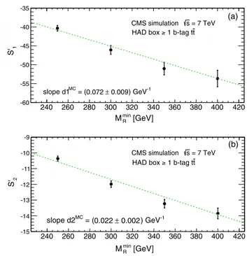
In both the simulated and the data events in the MU and ELE razor boxes, the MR distribution is well described by
the sum of two exponential components. One component, which we denote the “first” component, has a steeper slope than the other, “second” component, i.e., jS1j > jS2j, and
thus the second component is dominant in the high-MR
region. The relative normalization of the two components is considered as an additional degree of freedom. Both the S1
and S2 values, along with their relative and absolute
normalizations, are determined in the fit. The MR
distributions are shown as a function of R2
min in Fig. 5
for the zero b-jet MU data, which is dominated by W þ jets events. The dependence of S1 and S2 on R2min is shown
in Fig.6.
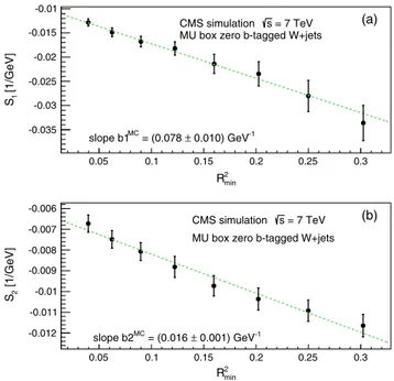
The corresponding results from simulation are shown in Figs. 7 and 8. It is seen that the values of the slope parameters b1 and b2 from simulation, given in Fig. 8,
agree within the uncertainties with the results from data, given in Fig.6.
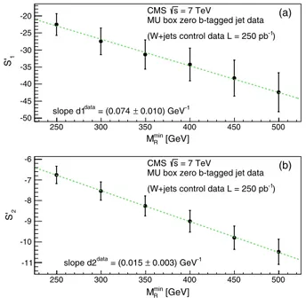
The R2distributions as a function of Mmin
R for the data are
shown in Fig.9for the MU box with the requirement of zero b-tagged jets. The S0
1and S02parameters characterizing
the exponential behavior of the first and second WðμνÞ þ jets components are shown in Fig.10. The corresponding
[GeV] R M 200 300 400 500 600 700 Events /(26 GeV) 2 10 > 0.04 2 R > 0.06 2 R > 0.09 2 R > 0.12 2 R > 0.16 2 R > 0.20 2 R > 0.25 2 R > 0.30 2 R = 7 TeV s CMS
MU box zero b-tagged jet data ) -1 (W+jets control data, L = 250 pb
FIG. 5 (color online). The MRdistribution for different values of R2
minfor events in the MU box, with the requirement of zero b-tagged jets. The curves show the results of fits of a sum of two exponential distributions. 2 min R 0.05 0.1 0.15 0.2 0.25 0.3 [1/GeV]1 S -0.04 -0.035 -0.03 -0.025 -0.02 -0.015 = 7 TeV s CMS
MU box zero b-tagged jet data )
-1
(W+jets control data L = 250 pb
-1 0.010) GeV ± = (0.081 data slope b1 (a) min 2 R 0.05 0.1 0.15 0.2 0.25 0.3 [1/GeV]2 S -0.013 -0.012 -0.011 -0.01 -0.009 -0.008
-0.007 CMSMU box zero b-tagged jet datas = 7 TeV
)
-1
(W+jets control data L = 250 pb
-1 0.001) GeV ± = (0.016 data slope b2 (b)
FIG. 6 (color online). Value of (a) the coefficient in the first exponent, S1, and (b) the coefficient in the second exponent, S2, from fits to the MRdistribution, as a function of R2min, for events in the MU box, with the requirement of zero b-tagged jets.
[GeV] R M 200 300 400 500 600 700 800 900 1000 Events / (26 GeV) 2 10 3 10 > 0.04 2 R > 0.06 2 R > 0.09 2 R > 0.12 2 R > 0.16 2 R > 0.20 2 R > 0.25 2 R > 0.30 2 R = 7 TeV s CMS simulation
MU box zero b-tagged W+jets
FIG. 7 (color online). The MRdistributions for different values of R2
min for W þ jets simulated events in the MU box with the requirement of zero b-tagged jets. The curves show the results of fits of a sum of two exponential distributions.
min 2 R 0.05 0.1 0.15 0.2 0.25 0.3 [1/GeV]1 S -0.035 -0.03 -0.025 -0.02 -0.015 -0.01 = 7 TeV s CMS simulation
MU box zero b-tagged W+jets
-1 0.010) GeV ± = (0.078 MC slope b1 (a) min 2 R 0.05 0.1 0.15 0.2 0.25 0.3 [1/GeV]2 S -0.012 -0.011 -0.01 -0.009 -0.008 -0.007 -0.006 = 7 TeV s CMS simulation
MU box zero b-tagged W+jets
-1 0.001) GeV ± = (0.016 MC slope b2 (b)
FIG. 8 (color online). Value of (a) the coefficient in the first exponent, S1, and (b) the coefficient in the second exponent, S2, from fits to the MR distribution, as a function of R2min, for simulated W þ jets events in the MU box with the requirement of zero b-tagged jets.
results from simulation are shown in Figs.11and12. The results for the slopes d1 and d2 from simulation, listed in
Fig. 12, are seen to be in agreement with the measured results, listed in Fig.10. Furthermore, the extracted values of d1and d2are in agreement with the extracted values of
b1and b2, respectively. This is the essential ingredient to
build a 2D template for the (MR,R2) distributions, starting
with the function of Eq.(5).
The corresponding distributions for the t¯t MC simulation with ≥1 b-tagged jet are presented in Appendix A, for events selected in the HAD box.
C. Dilepton backgrounds
The SM contributions to the ELE-ELE and MU-MU boxes are expected to be dominated by Z þ jets events, and the SM contribution to the ELE-MU box by t¯t events, all at the level of≳95%. We find that the MR distributions as a
function of R2
min, and the R2 distribution as a function of
Mmin
R , are independent of the lepton-flavor combination for
both the ELE-ELE and MU-MU boxes, as determined using simulated t¯tð2l2ν þ jetsÞ events. In addition, the asymptotic second component is found to be process independent. 2 R 0.1 0.15 0.2 0.25 0.3 0.35 0.4 0.45 0.5 Events /(0.008) 10 > 250 GeV R M > 300 GeV R M > 350 GeV R M > 400 GeV R M = 7 TeV s CMS
MU box zero b-tagged jet data )
-1
(W+jets control data L = 250 pb
FIG. 9 (color online). The R2distributions for different values of Mmin
R for events in the MU box, with the requirement of zero b-tagged jets. The curves show the results of fits of a sum of two exponential distributions. [GeV] min R M 250 300 350 400 450 500 1 S -50 -45 -40 -35 -30 -25
-20 CMSMU box zero b-tagged jet datas = 7 TeV
)
-1
(W+jets control data L = 250 pb
-1 0.010) GeV ± = (0.074 data slope d1 (a) [GeV] min R M 250 300 350 400 450 500 2 S -11 -10 -9 -8 -7 -6 CMS s = 7 TeV
MU box zero b-tagged jet data )
-1
(W+jets control data L = 250 pb
-1 0.003) GeV ± = (0.015 data slope d2 (b)
FIG. 10 (color online). Value of (a) the coefficient in the first exponent, S0
1, and (b) the coefficient in the second exponent, S02, from fits to the R2distribution, as a function of Mmin
R , for events in the MU box, with the requirement of zero b-tagged jets.
2 R 0.1 0.15 0.2 0.25 0.3 0.35 0.4 0.45 0.5 Events /(0.008) 2 10 > 250 GeV R M > 300 GeV R M > 350 GeV R M > 400 GeV R M = 7 TeV s CMS simulation
MU box zero b-tagged W+jets
FIG. 11 (color online). The R2distributions for different values of Mmin
R for W þ jets simulated events in the MU box with the requirement of zero b-tagged jets. The curves show the results of fits of a sum of two exponential distributions.
[GeV] min R M 250 300 350 400 450 500 1 S -50 -45 -40 -35 -30 -25 -20 CMS simulation s = 7 TeV
MU box zero b-tagged W+jets
-1 0.008) GeV ± = (0.071 MC slope d1 (a) [GeV] min R M 250 300 350 400 450 500 2 S -11 -10 -9 -8 -7 -6 = 7 TeV s CMS simulation
MU box zero b-tagged W+jets
-1 0.002) GeV ± = (0.019 MC slope d2 (b)
FIG. 12 (color online). Value of (a) the coefficient in the first exponent, S0
1, and (b) the coefficient in the second exponent, S02, from fits to the R2distribution, as a function of Mmin
R , for W þ jets simulated events in the MU box with the requirement of zero b-tagged jets.
VI. Background model and fits
As described earlier, the full 2D SM background representation is built using statistically independent data control samples. The parameters of this model provide the input to the final fit performed in the fit region (FR) of the data samples, defining an extended, unbinned maximum likelihood (ML) fit with the ROOFITfitting package [63].
The fit region is defined for each of the razor boxes as the region of low MRand small R2, where signal contamination
is expected to have negligible impact on the shape fit. The 2D model is extrapolated to the rest of the (MR, R2) plane,
which is sensitive to new-physics signals and where the search is performed.
For each box, the fit is conducted in the signal-free FR of the (MR, R2) plane; their definition can be found in
Figs. 15,17, 19, 21, 23, and 25. These regions are used to provide a full description of the SM background in the entire (MR, R2) plane in each box. The likelihood function
for a given box is written as[64]
Lb¼e −$Pj∈SMNj % N! YN i¼1 & X j∈SM NjPjðMR;i; R2iÞ ' ; ð8Þ
where N is the total number of events in the FR region of the box, the sum runs over all the SM processes relevant for that box, and the Njare normalization parameters for each
SM process involved in the considered box.
We find that each SM process in a given final-state box is well described in the (MR, R2) plane by the function Pj
defined as
PjðMR; R2Þ ¼ ð1 − fj2Þ × F1stj ðMR; R2Þ þ fj2
× F2nd
j ðMR; R2Þ; ð9Þ
where the first (F1st
j ) and second (F2ndj ) components are
defined as in Eq.(5), and fj2is the normalization fraction of the second component with respect to the total. When fitting this function to the data, the shape parameters of each FjðMR; R2Þ function, the absolute normalization, and the
relative fraction fj2are floated in the fit. Studies of simulated events and fits to data control samples with either a b-jet requirement or a b-jet veto indicate that the parameters corresponding to the first components of these backgrounds (with steeper slopes at low MR and R2) are box dependent.
The parameters describing the second components are box independent, and at the current precision of the background model, they are identical between the dominant backgrounds considered in these final states.
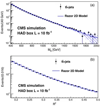
We validate the choice of the background shape by use of a sample of t¯t MC simulated events corresponding to an integrated luminosity of 10 fb−1. Besides being the
dom-inant background in the≥1 b-tag search, t¯t events are the dominant background for the inclusive search for large
values of MR and R2. The result for the HAD box in the
inclusive razor path is shown in Fig.13 expressed as the projection of the 2D fit on MRand R2. As the same level of
agreement is found in all boxes both in the inclusive and in the≥1 b-tagged razor path, we proceed to fit all the SM processes with this shape.
A. Fit results and validation
The shape parameters in Eq.(5)are determined for each box via the 2D fit. The likelihood of Eq.(8)is multiplied by Gaussian penalty terms[65]to account for the uncertainties of the shape parameters kj, M0R;j, and R20;j. The central
values of the Gaussians are derived from analogous 2D fits in the low-statistics data control sample. The penalty terms pull the fit to the local minimum closer to the shape derived from the data control samples. Using pseudoexperiments, we verified that this procedure does not bias the determi-nation of the background shape. As an example, the kj
parameter uncertainties are typically ∼30%. Additional background shape uncertainties due to the choice of the functional form were considered and found to be negli-gible, as discussed in AppendixB.
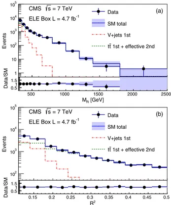
The result of the ML fit projected on MRand R2is shown
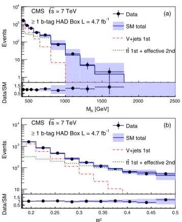
in Fig. 14 for the inclusive HAD box. No significant discrepancy is observed between the data and the fit model for any of the six boxes. In order to establish the
[GeV] R M 400 600 800 1000 1200 1400 1600 1800 2000 Events/(40 GeV) -1 10 1 10 2 10 3 10 4 10 5 10 +jets t t Razor 2D Model CMS simulation -1 HAD box L = 10 fb (a) 2 R 0.2 0.25 0.3 0.35 0.4 0.45 0.5 Events/(0.016) 3 10 4 10 +jets t t Razor 2D Model CMS simulation -1 HAD box L = 10 fb (b)
FIG. 13 (color online). Projection of the 2D fit result on (a) MR and (b) R2for the HAD box in t¯t MC simulation. The continuous histogram is the 2D model prediction obtained from a single pseudo-experiment based on the 2D fit. The fit is performed in the (MR, R2) fit region and projected into the full analysis region. Only the statistical uncertainty band in the background prediction is drawn in these projections. The points show the distribution for the MC simulated events.
compatibility of the background model with the observed data set, we define a set of signal regions (SRi) in the tail of the SM background distribution. Using the 2D back-ground model determined using the ML fit, we derive the distribution of the expected yield in each SRi using pseudoexperiments, accounting for correlations and uncer-tainties in the parameters describing the background model. In order to correctly account for the uncertainties in the parameters describing the background model and their correlations, the shape parameters used to generate each pseudoexperiment data set are sampled from the covariance matrix returned by the ML fit performed on the actual data set. The actual number of events in each data set is drawn from a Poisson distribution centered on the yield returned by the covariance matrix sampling. For each pseudoexperi-ment data set, the number of events in the SRi is found. For each of the SRi, the distribution of the number of events derived by the pseudoexperiments is used to calculate a two-sided p-value (as shown for the HAD box in Fig.15), corresponding to the probability of observing an equal or less probable outcome for a counting experiment in each signal region. The result of the ML fit and the correspond-ing p-values are shown in Figs.16and17for the ELE box,
Figs.18and19for the MU box, Figs. 20and21 for the ELE-ELE box, Figs.22and23for the MU-MU box, and Figs. 24 and 25 for the MU-ELE box. We note that the background shapes in the single-lepton and hadronic boxes
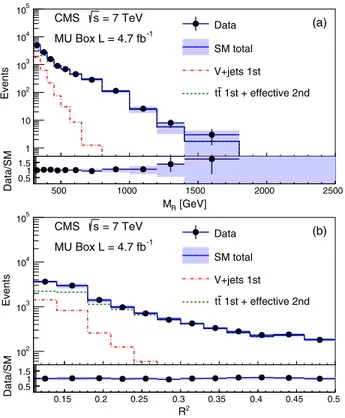
Events 1 10 2 10 3 10 4 10 5 10 Data SM total V+jets 1st 1st + effective 2nd t t = 7 TeV s CMS -1 HAD Box L = 4.7 fb [GeV] R M 500 1000 1500 2000 2500 Data/SM 0.51 1.5 (a) Events 2 10 3 10 4 10 5 10 Data SM total V+jets 1st 1st + effective 2nd t t = 7 TeV s CMS -1 HAD Box L = 4.7 fb 2 R 0.2 0.25 0.3 0.35 0.4 0.45 0.5 Data/SM 0.5 1 1.5 (b)
FIG. 14 (color online). Projection of the 2D fit result on (a) MR and (b) R2for the inclusive HAD box. The continuous histogram is the total SM prediction. The dash-dotted and dashed histograms are described in the text. The fit is performed in the (MR, R2) fit region (shown in Fig. 15) and projected into the full analysis region. The full uncertainty in the total background prediction is drawn in these projections, including the one due to the variation of the background shape parameters and normalization.
FIG. 15 (color online). The fit region, FR, and signal regions, SRi, are defined in the (MR, R2) plane for the HAD box. The color scale gives the p-values corresponding to the observed number of events in each SRi, computed from background parametrization derived in the FR. The p-values are also given in the table, together with the observed number of events, the median and the mode of the yield distribution, and a 68% C.L. interval.
Events 1 10 2 10 3 10 4 10 5 10 Data SM total V+jets 1st 1st + effective 2nd t t = 7 TeV s CMS -1 ELE Box L = 4.7 fb (a) [GeV] R M 500 1000 1500 2000 2500 Data/SM 0.51 1.5 Events 2 10 3 10 4 10 5 10 Data SM total V+jets 1st 1st + effective 2nd t t = 7 TeV s CMS -1 ELE Box L = 4.7 fb (b) 2 R 0.15 0.2 0.25 0.3 0.35 0.4 0.45 0.5 Data/SM 0.5 1 1.5
FIG. 16 (color online). Projection of the 2D fit result on (a) MR and (b) R2for the inclusive ELE box. The fit is performed in the (MR, R2) fit region (shown in Fig.17) and projected into the full analysis region. The histograms are described in the text.
are well described by the sum of two functions: a single-component function with a steeper-slope single-component, denoted as the V þ jets first component, obtained by fixing f2¼ 0 in Eq. (9); and a two-component function as in
Eq. (9), with the first component describing the steeper-slope core of the t¯t and single-top background distributions
(generically referred to as t¯t), and the effective second component modeling the sum of the indistinguishable tails of different SM background processes. In the dilepton boxes we show the total SM background, which is composed of V þ jets and t¯t events in the ELE-ELE and MU-MU boxes and of t¯t events in the MU-ELE boxes. The
FIG. 17 (color online). The fit region, FR, and signal regions, SRi, are defined in the (MR, R2) plane for the ELE box. The color scale gives the p-values corresponding to the observed number of events in each SRi. Further explanation is given in the Fig.15 caption. Events 1 10 2 10 3 10 4 10 5 10 Data SM total V+jets 1st 1st + effective 2nd t t = 7 TeV s CMS -1 MU Box L = 4.7 fb (a) [GeV] R M 500 1000 1500 2000 2500 Data/SM 0.5 1 1.5 Events 2 10 3 10 4 10 5 10 Data SM total V+jets 1st 1st + effective 2nd t t = 7 TeV s CMS -1 MU Box L = 4.7 fb (b) 2 R 0.15 0.2 0.25 0.3 0.35 0.4 0.45 0.5 Data/SM 0.5 1 1.5
FIG. 18 (color online). Projection of the 2D fit result on (a) MR and (b) R2for the inclusive MU box. The fit is performed in the (MR, R2) fit region (shown in Fig.19) and projected into the full analysis region. The histograms are described in the text.
FIG. 19 (color online). The fit region, FR, and signal regions, SRi, are defined in the (MR, R2) plane for the MU box. The color scale gives the p-values corresponding to the observed number of events in each SRi. Further explanation is given in the Fig.15 caption. Events 1 10 2 10 3 10 Data SM total = 7 TeV s CMS -1 ELE-ELE Box L = 4.7 fb (a) [GeV] R M 500 1000 1500 2000 2500 Data/SM 0.5 1 1.5 Events 1 10 2 10 3 10 Data SM total = 7 TeV s CMS -1 ELE-ELE Box L = 4.7 fb (b) 2 R 0.15 0.2 0.25 0.3 0.35 0.4 0.45 0.5 Data/SM 0.5 1 1.5
FIG. 20 (color online). Projection of the 2D fit result on (a) MR and (b) R2 for the ELE-ELE box. The continuous histogram is the total standard model prediction. The histogram is described in the text.
corresponding results for the ≥1 b-tagged samples are presented in AppendixC.
VII. SIGNAL SYSTEMATIC UNCERTAINTIES We evaluate the impact of systematic uncertainties on the shape of the signal distributions, for each point of each SUSY
model, using the simulated signal event samples. The follow-ing systematic uncertainties are considered, with the approxi-mate size of the uncertainty given in parentheses: (i) PDFs (up to 30%, evaluated point by point)[66]; (ii) jet-energy scale (up to 1%, evaluated point by point)[43]; (iii) lepton identifica-tion, using the “tag-and-probe” technique based on Z → ll events [67] (l ¼ e; μ, 1% per lepton). In addition, the
FIG. 21 (color online). The fit region, FR, and signal regions, SRi, are defined in the (MR, R2) plane for the ELE-ELE box. The color scale gives the p-values corresponding to the observed number of events in each SRi. Further explanation is given in the Fig.15 caption. Events 1 10 2 10 3 10 Data SM total = 7 TeV s CMS -1 MU-MU Box L = 4.7 fb (a) [GeV] R M 500 1000 1500 2000 2500 Data/SM 0.5 1 1.5 Events 10 2 10 3 10 Data SM total = 7 TeV s CMS -1 MU-MU Box L = 4.7 fb (b) 2 R 0.15 0.2 0.25 0.3 0.35 0.4 0.45 0.5 Data/SM 0.5 1 1.5
FIG. 22 (color online). Projection of the 2D fit result on (a) MR and (b) R2for the inclusive MU-MU box. The fit is performed in the (MR, R2) fit region (shown in Fig.23) and projected into the full analysis region. The histogram is described in the text.
FIG. 23 (color online). The fit region, FR, and signal regions, SRi, are defined in the (MR, R2) plane for the MU-MU box. The color scale gives the p-values corresponding to the observed number of events in each SRi. Further explanation is given in the Fig.15caption. Events 1 10 2 10 3 10 Data SM total = 7 TeV s CMS -1 MU-ELE Box L = 4.7 fb (a) [GeV] R M 400 600 800 1000 1200 1400 1600 1800 Data/SM0.5 1 1.5 Events 1 10 2 10 3 10 Data SM total = 7 TeV s CMS -1 MU-ELE Box L = 4.7 fb (b) 2 R 0.15 0.2 0.25 0.3 0.35 0.4 0.45 0.5 Data/SM0.5 1 1.5
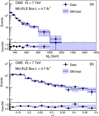
FIG. 24 (color online). Projection of the 2D fit result on (a) MR and (b) R2for the inclusive MU-ELE box. The fit is performed in the (MR, R2) fit region (shown in Fig.25) and projected into the full analysis region. The histogram is described in the text.
following uncertainties, which affect the signal yield, are considered: (i) luminosity uncertainty[68](2.2%); (ii) theo-retical cross section[69](up to 15%, evaluated point by point); (iii) razor trigger efficiency (2%); (iv) lepton trigger efficiency (3%). An additional systematic uncertainty is considered for the b-tagging efficiency[49] (between 6% and 20% in pT
bins). We consider variations of the function modeling, the signal uncertainty (log normal versus Gaussian), and the binning, and find negligible deviations in the results. The systematic uncertainties are included using the best-fit shape to compute the likelihood values for each pseudoexperiment, while sampling the same pseudoexperiment from a different function, derived from the covariance matrix of the fit to the data. This procedure is repeated for both the background and signal probability density functions.
VIII. INTERPRETATION OF THE RESULTS In order to evaluate exclusion limits for a given SUSY model, its parameters are varied and an excluded cross
FIG. 25 (color online). The fit region, FR, and signal regions, SRi, are defined in the (MR, R2) plane for the MU-ELE box. The color scale gives the p-values corresponding to the observed number of events in each SRi. Further explanation is given in the Fig.15 caption. [GeV] 0 m 500 1000 1500 2000 2500 3000 [GeV] 1/2 m 100 200 300 400 500 600 700 800 900 1000 ± l ~ LEP2 ± 1 χ∼ LEP2 No EWSB = LSPτ∼ Non-Convergent RGE's ) = 500 g~ m( ) = 1000 g~ m( ) = 1500 g~ m( ) = 2000 g~ m( ) = 1000 q~ m( ) = 1500 q~ m( ) = 2000 q~ m(
Median expected limit σ 1 ± Expected limit Observed limit -1 = 7 TeV, L = 4.7 fb s CMS Hybrid CLs 95% C.L. limits Razor inclusive No EWSB Non-Convergent RGE's )=10 β tan( = 0 GeV 0 A > 0 µ = 173.2 GeV t m = LSPτ∼ [GeV] 0 m 500 1000 1500 2000 2500 3000 [GeV] 1/2 m 100 200 300 400 500 600 700 800 900 1000 ± l ~ LEP2 ± 1 χ∼ LEP2 No EWSB = LSPτ∼ Non-Convergent RGE's ) = 500 g~ m( ) = 1000 g~ m( ) = 1500 g~ m( ) = 2000 g~ m( ) = 1000 q~ m( ) = 1500 q~ m( ) = 2000 q~ m(
Median expected limit σ 1 ± Expected limit Observed limit HAD observed limit Leptons observed limit
-1 = 7 TeV, L = 4.7 fb s CMS Hybrid CLs 95% C.L. limits Razor inclusive No EWSB Non-Convergent RGE's )=10 β tan( = 0 GeV 0 A > 0 µ = 173.2 GeV t m = LSPτ∼ [GeV] 0 m 500 1000 1500 2000 2500 3000 [GeV] 1/2 m 100 200 300 400 500 600 700 800 900 1000 ± l ~ LEP2 ± 1 LEP2 No EWSB = LSP Non-Convergent RGE's ) = 500 g~ m( ) = 1000 g~ m( ) = 1500 g~ m( ) = 2000 g~ m( ) = 1000 q~ m( ) = 1500 q~ m( ) = 2000 q~ m( ) = 2500 q~ m(
HAD expected limit 1 ± HAD exp. limit HAD observed limit
-1 L dt = 4.7 fb = 7 TeV s CMS Razor Inclusive No EWSB Non-Convergent RGE's )=10 tan( = 0 GeV 0 A > 0 µ = 173.2 GeV t m = LSP -1 L = 4.7 fb Razor i -1 = 7 TeV, L = 4.7 fb s CMS [GeV] 0 m 500 1000 1500 2000 2500 3000 [GeV] 1/2 m 100 200 300 400 500 600 700 800 900 1000 ± l ~ LEP2 ± 1 LEP2 No EWSB = LSP Non-Convergent RGE's ) = 500 g~ m( ) = 1000 g~ m( ) = 1500 g~ m( ) = 2000 g~ m( ) = 1000 q~ m( ) = 1500 q~ m( ) = 2000 q~ m( ) = 2500 q~ m(
Leptons expected limit 1 ± Leptons exp. limit Leptons observed limit
-1 L dt = 4.7 fb = 7 TeV s CMS Razor Inclusive No EWSB Non-Convergent RGE's )=10 tan( = 0 GeV 0 A > 0 µ = 173.2 GeV t m = LSP -1 L = 4.7 fb Razor i -1 = 7 TeV, L = 4.7 fb s CMS
Hybrid CLs 95% C.L. limits Hybrid CLs 95% C.L. limits
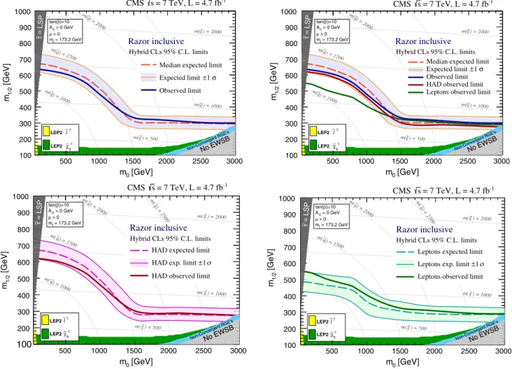
FIG. 26 (color online). (Upper left panel) Observed (solid curve) and median expected (dashed orange curve) 95% C.L. limits in the (m0, m1=2) CMSSM plane (drawn according to Ref.[73]) with tan β ¼ 10, A0¼ 0, and sgnðμÞ ¼ þ1. The (1 standard deviation equivalent variations due to the uncertainties are shown as a band around the median expected limit. (Upper right panel) The observed HAD-only (solid red) and leptonic-only (solid green) 95% C.L. limits are shown, compared to the combined limit (solid blue curve). The expected (dashed curve) and observed (solid curve) limits for the (lower left) HAD-only and (lower right) leptonic boxes only are also shown.
section at the 95% C.L. is associated with each configu-ration of the model parameters, using the hybrid version of the CLs method[70–72], described below.
For each box, we consider the test statistic given by the logarithm of the likelihood ratio ln Q ¼ ln½Lðs þ bjHiÞ=LðbjHiÞ&, where Hiði ¼ 0; 2Þ is the hypothesis
under test: H1(signal plus background) or H0(background
only). The likelihood function for the background-only hypothesis is given by Eq.(8). The likelihood correspond-ing to the signal-plus-background hypothesis is written as
Lsþb¼e −$Pj∈SMNj % N! YN i¼1 & X j∈SM NjPjðMR;i; R2iÞ þ σ × L × ϵPSðMR;i; R2iÞ ' ; ð10Þ
where σ is the signal cross section, i.e., the parameter of interest; L is the integrated luminosity; ϵ is the signal acceptance times efficiency; and PSðMR;i; R2iÞ is the
two-dimensional probability density function for the signal, computed numerically from the distribution of simulated signal events. The signal and background shape parameters, and the normalization factors L and ϵ, are the nuisance parameters.
For each analysis (inclusive razor or inclusive b-jet razor) we sum the test statistics of the six corresponding boxes to compute the combined test statistic.
The distribution of ln Q is derived numerically with an MC technique. The values of the nuisance parameters in the likelihood are randomized for each iteration of the MC generation, to reflect the corresponding uncertainty. Once the likelihood is defined, a sample of events is generated according to the signal and background probability density functions. The value of ln Q for each generated sample is then evaluated, fixing each signal and background param-eter to its expected value. This procedure corresponds to a numerical marginalization of the nuisance parameters.
Given the distribution of ln Q for the background-only and the signal-plus-background pseudoexperiments, and