Entanglement and squeezing of continuous-wave stationary light

PAPER • OPEN ACCESS

Entanglement and squeezing of continuous-wave

stationary light

To cite this article: Stefano Zippilli et al 2015 New J. Phys. 17 043025

View the article online for updates and enhancements.

Related content

Large distance continuous variable communication with concatenated swaps

Muhammad Asjad, Stefano Zippilli, Paolo Tombesi et al.

-Entangling the motion of two optically trapped objects via time-modulated driving fields

Mehdi Abdi and Michael J Hartmann

-Strong squeezing via phonon mediated spontaneous generation of photon pairs

Kenan Qu and G S Agarwal

-Recent citations

Suppression of Stokes scattering and improved optomechanical cooling with squeezed light

Muhammad Asjad et al

-Complex Squeezing and Force Measurement Beyond the Standard Quantum Limit

L. F. Buchmann et al

-Dynamical Two-Mode Squeezing of Thermal Fluctuations in a Cavity Optomechanical System

A. Pontin et al

PAPER

Entanglement and squeezing of continuous-wave stationary light

Stefano Zippilli, Giovanni Di Giuseppe and David Vitali

School of Science and Technology, Physics Division, University of Camerino, via Madonna delle Carceri, 9, I-62032 Camerino (MC), Italy INFN, Sezione di Perugia, Italy

E-mail:stefano.zippilli@unicam.it

Keywords: entanglement, squeezing, continuousfields, continuous variables, optomechanics

Abstract

Spectral components of continuous squeezed

fields are entangled. In this article we review and clarify

this phenomenon by analyzing systematically the relations between the correlations of modes

filtered

from stationary continuous

fields and the cross-power spectrum between the operators of the

corresponding spectral components. Moreover, we study the specific spectral components that are

filtered in homodyne or heterodyne detections and their entanglement properties. In particular, we

establish the equivalence between two-mode squeezing variance and logarithmic negativity for the

spectral components of continuous stationary

fields, thereby demonstrating that the measurement of

the homodyne or heterodyne spectrum is, in fact, a direct measurement of the logarithmic negativity

between specific spectral modes. As an illustrative example, we apply these concepts to the analysis of

entanglement in ponderomotive squeezing.

1. Introduction

Quantum opticalfields are exploited in the development of a large class of new technologies which make use of quantum mechanics to push their efficiency to the limit [1]. In particular, squeezed light plays a pivotal role in the continuous-variable domain [2–5]. After thefirst experimental demonstrations of optical squeezing, both in the continuous-wave [6,7] and in the pulsed regime [8], and of the corresponding Einstein–Podolsky–Rosen

(EPR) entanglement [9–11], nowadays squeezed opticalfields are routinely produced and employed in many experiments aimed at investigating the potentiality of quantum-based technologies. They range, for example, from the demonstration of quantum information tasks such as quantum teleportation [12,13] and other essential elements of scalable universal quantum computation [14–18] to the design of high-resolution metrology applications [19–23], of novel spectroscopic methods [24,25], and of enhanced optical communication schemes [26].

Squeezing and entanglement are two very related concepts. In practice squeezedfields are, for example, used to produce two-mode entangled resources by simply mixing them on beam splitters [10,12,16]. From a more theoretical point of view, squeezing variance can be used to construct entanglement criteria [27–30]. It is also well known that the spectral components of continuous-wave squeezed light are endowed with non-trivial correlations [31–35]. In particular, specific spectral modes of continuous squeezed fields are entangled [36–39], realizing EPR spectral beams that have been proposed as convenient quantum communication

channels [37,40].

In this article we study squeezed continuousfields in the stationary regime, and we analyze the entanglement properties of the corresponding spectral components. We aim at establishing a direct connection between the entanglement theory of continuous-variable systems and the spectral properties of squeezed lightfields in the stationary continuous-wave regime. The spectral modes of a continuousfield can be operatively defined as the temporal modesfiltered from the total field, with a long time filter. Their entanglement and squeezing properties are therefore readily defined as the long time limit of those that are found for finite temporal modes. By

employing this approach, we derive general conditions for entanglement and squeezing between two spectral components of stationary continuousfields, and we show that their two-mode squeezing variance can be expressed in terms of the corresponding logarithmic negativity. We also discuss the properties of the specific

OPEN ACCESS

RECEIVED

20 November 2014

REVISED

11 February 2015

ACCEPTED FOR PUBLICATION

12 March 2015

PUBLISHED

15 April 2015

Content from this work may be used under the terms of theCreative Commons Attribution 3.0 licence.

Any further distribution of this work must maintain attribution to the author(s) and the title of the work, journal citation and DOI.

spectral modes that are probed with homodyne and heterodyne detection [41,42], and we establish that the squeezing spectrum that can be measured with these techniques can be interpreted as a direct measurement of the logarithmic negativity between specific spectral modes.

Finally, we apply these ideas to the analysis of ponderomotive squeezing [43–46], namely the squeezing that is obtained as a result of the optomechanical interaction between a mechanical resonator and the light in an optical cavity. Optomechanics provides a novel approach to the area of quantum non-linear optics, which recently has attracted much attention for its potential applications in quantum-enhanced technologies [47,48]. In this work, we investigate a two-sided cavity with a membrane in the middle, and we identify the spectral components of the outputfields that exhibit larger entanglement and that are experimentally accessible with homodyne and heterodyne techniques.

Part of this article comprises a review of already known results, however, rephrased with the intent of providing a clear and complete introduction to the scope of our research. In particular, in our presentation, the revision of established concepts is instrumental to the identification and full understanding of the new results concerning the relationship between entanglement and squeezing in continuous stationaryfields that constitute the central outcome of this article. In detail, the article is organized as follows. In section2we review the basic properties of continuousfields and of their spectral properties. We introduce the filtered temporal modes and study the correlations of the correspondingfield operators in the stationary regime. In section3we demonstrate the equivalence between logarithmic negativity and two-mode squeezing variance of the spectral components of stationary continuousfields. In section4we review homodyne and heterodyne detection techniques and study how they can be used to directly measure the logarithmic negativity between spectral modes. Then, in section5, we apply the concepts developed in the preceding sections to ponderomotive squeezing. Finally, in section6, we draw our conclusions and discuss some possible outlooks. The three appendices provide additional information regarding, respectively, the basic properties of entanglement and squeezing of discrete bosonic modes, the homodyne and heterodyne techniques, and the input–output theory applied to the investigation of an optomechanical system.

2. Continuous quantum optical

fields

In this section we introduce the objects of our investigation, namely continuousfields, and we discuss the properties of temporal modes that can befiltered from them [49–51]. In particular we define the operators for the spectral components in terms of the modes that arefiltered with a long-time filter and that describe narrow bands of frequencies. These operators are particularly suited for the study of the entanglement properties of the spectral components of continuousfields using standard techniques of entanglement theory.

In detail, we investigate the freely propagating continuousfield E(t) at the output of a quantum optical system. It can be decomposed into the positive and negative frequency componentsE t( )= E( )+ ( )t +E( )− ( )t _,

with =

∫

ω ω ω πϵ σ ω + ∞ − E ( )t i d e a( ) c kz t ( ) 0 4 i( ) 0

and_E( )−_{( )t} =

{

_E( )+_{( )t}

}

†_{, whereσ is the cross section of the}

propagatingfield and ωa ( ) is the annihilation operator for the spectral component at frequencyω that satisfy the standard commutation relation⎡⎣a( ), { (ω a ω′)}†⎤⎦=δ ω( −ω′)_{. In general, in an optical system, only a} relatively narrow band of frequenciesΔωis relevant. This band is centered around the carrier frequencyωLof

the signalfield E(t), which is typically defined by the frequency of a laser driving the system and fulfills the relation Δω ≪ωL. In practice the relevant bandwidth is set by the typical line widthΓ of the system under

investigation and eventually by the response time, T, of the detector such that Γ{ , 1 T}≪Δω. Under these

conditions the range of frequency integration in the expression for thefield can be extended from −∞ to ∞, and the relevant wave numbers k can be approximated with the central valuek∼ωL c=kL. By this means the

quantum optical continuousfield can be expressed as ω ϵ σ = + E t c a t ( ) i 2 e ( ), (1) L _{k z} ( ) 0 iL

where we have introduced the continuousfield annihilation operator a(t). It is related to the operators for the

spectral components by the Fourier transform = _π

∫

ω ω ω ω +ω

−∞ ∞ _{− +} a t( ) d e ta( ) L 1 2

i( L ) _{, where here}ω is the

frequency relative to the carrier. It is also useful to introduce the operators_a∼_{( )}ω =_a(ω + ω_)e−ω

L i Ltrelative to

the carrier frequency, which are equal to the Fourier transform of a(t):

∫

ω π = ∼ ω −∞ ∞ a( ) 1 t a t 2 d e ( ), (2) t i

and

{

a∼( )ω

}

† =a͠†(−ω)_{. These operators satisfy the standard commutation relation for continuousfields:} ω ω δ ω ω δ ′ = + ′ ′ = − ′ ∼ ͠ a a a t a t t t ( ), ( ) ( ) ( ), ( ) ( ). (3) † † ⎡ ⎣ ⎤⎦ ⎡⎣ ⎤⎦

2.1. Filtered modes and spectral components of thefield

In reality one has access only to afinite time interval (and correspondingly to a finite band of frequencies) of the totalfield a(t). These detectable intervals of the total field correspond to specific temporal modes. They can be physically defined, for example, by the temporal profile of the pumping field in pulsed experiments [8,10,52– 54], they can also be extracted by post-processing the previously recorded time signal [55,56], or they can be selected by the measurement apparatus as a result of the corresponding response and detection times [56–59]. In particular, in the case of experiments involving stationaryfields, the detection time can be sufficiently long to select a well-defined spectral component of the total signal (as achieved, for example, with an electronic spectrum analyzer) [6,7,42].

In general a temporalfiltered mode can be introduced in terms of a filter function ϕ_τ( ), which defines thet time profile of the mode with a duration of order τ. Correspondingly, it defines a band of spectral components, of width1τ, that are combined into thefiltered signal [60,61]. The generic form for the operators of afiltered mode can be expressed as

∫

Ω = ϕ − τ Ω τ −∞ ∞ a ( , )t d es i s (t s a s) ( ) (4) with

{

aτ( , )Ω t

}

=aτ (−Ω, )t † _†

, and where the symbol indicatesfiltered quantities. The parameter Ω defines the central frequency of thefilter, and the filter functionϕ_τ( )t is real and normalized according to

∫

ϕτ =

−∞ ∞

s s

d ( )2 1. (5)

Consequently, thefiltered operators are discrete bosonic operators which satisfy the standard commutation relation Ω −Ω = ∀τ τ τ a ( , ),t a†( , )t 1, . ⎡ ⎣ ⎤⎦

The corresponding equivalent form of thefiltered operators, in terms of the spectral components of the field, is

∫

Ω = ω ϕ ω∼ −Ω ∼ ω τ ω Ω τ −∞ ∞ − − a ( , )t d e i( )t ( ) ( )a (6)

where ϕ ω∼τ( ) is the Fourier transformedfilter functionϕ ω =

∫

ϕ

∼ τ _{π −∞} ω τ ∞ s s ( ) 1 d e s ( ), 2 i _{which peaks at ω = 0}

and has a width on the order of1 τ.

Two particular cases are worth mentioning: the exponentialfilter with ϕ_τexp _{( )t} = _{2 ( )e}θ _t −tτ τ_and ϕ∼_τexp( )ω = τ π (1− iτ ω), which has been used, for example, in [57] to introduce the physical spectrum of light; and the step-filter function

ϕ θ θ τ τ ϕ ω π τ ω τ π ω = − ∼ = τ τ ωτ t t t ( ) ( ) ( ), ( ) 2 e sin( 2) (7) step step i ₂

which we will connect to homodyne and heterodyne detection techniques in the following. In this form the time t in thefiltered operatoraτ( , ) corresponds to theΩ t final time of the filtering process, that is,

∫

Ω = ϕ −

τ _−∞ Ω τ

a ( , )t t d es i s (t s a s) ( )._{Although not strictly relevant to the results presented in this article, this} choice is physically motivated by the fact that in this way we define, at time t, a causal operatoraτ( , ) whichΩ t depends only on the past of the continuousfield a(t) [60].

In the limit of longfiltering times,τ → ∞, thefilter selects a single spectral component of the field. In the following we will focus on the spectral components of stationaryfields for which we will use the following simplified notation:

Ω ≡ Ω

τ→∞ τ

a( ) lima ( , ),t (8)

where we drop the labelτ, the limit symbol, and the time argument t. In particular, the time t in these operators is irrelevant for stationaryfields, in the sense that (as shown in the next section) the correlations of operators of this form, in the limit of largeτ, are independent of the time arguments.

Wefinally note that we are describing the field in a reference frame rotating at the carrier frequencyωL;

thereforea ( ) is, in fact, the operator for the spectral component of theΩ field at the sideband frequency ωL +Ω.

2.2. Correlations offiltered spectral modes of stationary fields

In this article we are interested in the squeezing properties of the electromagneticfield, which refers to reduced fluctuations or reduced variance of specific quadratures below the vacuum noise level, and in the corresponding entanglement features. Squeezing can be revealed from the analysis of the second-order correlations offield operators. Therefore in this section we analyze the basic properties of the correlations offiltered modes. In particular we focus on the spectral properties of stationaryfields. The corresponding field operators, a(t) and

ω

∼

a( ), have diverging correlation functions as a consequence of the commutation relations in equation (3). In this case it is therefore instructive to analyze thefluctuations of the spectral modes in terms of the filtered spectral operators defined in equation (6), whose correlations, in contrast, are alwaysfinite also in the limit of long integration timeτ → ∞. This approach is particularly useful for the study of the corresponding entanglement properties, and it has the advantage of providing a clear physical definition of discrete modes corresponding to the specific spectral components, hence allowing for a transparent application of the techniques developed in entanglement theory, which indeed deals with discrete modes (see appendixA).

Let us study the correlations between the spectral components of two stationary continuousfields with annihilation operatorsa t1( )and a t2( )respectively, which fulfill the commutation relation

δ δ

′ = − ′

a tj( ),a tk( )† j k, (t t)

⎡⎣ ⎤⎦ . (The same results that we discuss hereafter for two continuousfields can be

applied with minor modifications to different spectral components belonging to a single field.) By straightforward application of the Wiener–Khintchine theorem, we find that all the information about the correlations between the spectral components is contained in the power spectrum matrix∼( ), defined as theω Fourier transform of the two-time stationary correlation matrix, which can be expressed in terms of the elements of the column vector of operatorsa( )t =

(

a t1( ), a t2( ),a1†( ),t a2†( )t

)

Tas the matrix

=

 t( ) a( ) (0)t a T _{, whose elements are{ t( )} = { ( )} { (0)}a t a}

j k, j k , wherej k, ∈{1, 2, 3, 4} are vector

indices, not to be confused with the indices of the modes. To be specific,

∫

ω = ∼ ω τ −∞ ∞ ( ) d et i ( ),t (9)

where we use the fact that two-time correlation functions of stationary signals depend only on the difference of the time arguments. In particular the correlations between the Fourier-transformed operators

∫

ω = ∼ π ω −∞ ∞ t t a( ) 1 d e ta( ) 2

i _{are diverging and are related to the power spectrum matrix by} ω ω′ =δ ω+ω′ ω

∼ ∼ ∼_

a( ) (a )T ( ) ( ). (10)

To gain insight into the physical meaning of these diverging quantities we employ the narrowfiltered modes introduced in the preceding section. We construct the vector offiltered spectral components

∫

Ω = τ→∞ _−∞ Ω ϕτ −

∞

s t s t

a( ) lim d ei s ( ) ( )a , which is given bya( )Ω =

(

a1( ),Ω a2( ),Ω a1†( ),Ω a2†( )Ω

)

T, and we compute the corresponding matrix of correlations:

∫

∫

Ω Ω′ = ω′ ω ∼ω ∼ω′ ϕ ω∼ −Ω ϕ ω∼ ′ −Ω′ τ ω Ω ω Ω τ τ →∞ −∞ ∞ −∞ ∞ − − + ′− ′ ′ a( ) (a )T lim d d a( ) (a )T e i[( )t ( ) ]t ( ) ( ). (11)

These quantities can be evaluated by noting that for largeτ, the square modulus of the filter function approaches a delta function,limτ→∞ ϕ ω∼τ( ) =δ ω( )

2

, whereas its integral goes to zero,limτ→∞

∫

dωϕ ω =∼τ( ) 0. And,

likewise, given a genericfinite function f ( )ω , the relation

∫

ωϕ ω∼ +Ω ϕ∼ −ω−Ω′ ω =δ Ω τ→∞ −∞ τ τ Ω Ω ∞ ′ f f lim d ( ) ( ) ( ) , ( ) (12)

holds. Consequently equations (10) and (12) can be used in equation (11) tofind Ω Ω′ =δΩ− ′Ω∼ Ω

a( ) (a )T ( ), (13)

,

which shows that the power spectrum is directly related to the correlations of narrowfiltered modes. In other terms, in the limit of large integration timeτ, i.e., when the bandwidth selected by the filter is sufficiently small, the correlation functions reduce to the power spectrum of the continuousfield [57]. This result is valid whenτ is much larger than the decay time of the signal correlationsτC(the memory time of the signals),τC≪τ. We note

in particular that this relation implies the stationarity of the signal, which is reached on a time scale on the order ofτC.

The correlations between two modes are conveniently analyzed in terms of the corresponding correlation matrix, from which the corresponding squeezing and entanglement properties can be readily derived (see appendixAfor a short review). We remark, however, that the matrix∼( ) is not a correlation matrix for twoΩ modes. In fact, it contains the correlations between the four spectral modes corresponding to the two pairs of sidebands at the frequency±Ωof the two continuousfields. On the other hand, the elements of the power spectrum matrix can be used to construct the correlation matrix for two narrow modesfiltered from the two stationary continuousfields as follows. We consider two modes, at frequencies Ω and Ω′, respectively described by thefiltered operators

Ω Ω Ω Ω − ′ − ′ a a a a ( ), ( ), ( ), ( ), (14) 1 1† 2 2†

where the narrow bandwidth limit τ → ∞( ) is implicit in their definition (see equation (8)). The corresponding correlation matrix is defined using the vector Ω Ωa( , ′ =)

(

a1( ),Ω a2(Ω′),a1†(−Ω), a2†(− ′Ω)

)

T, as

Ω Ω′ = Ω Ω′ Ω Ω′

( , ) a( , ) ( ,a )T _{, and can be expressed in terms of the elements of the power spectrum}

matrix defined in equation (13) as Ω Ω δ δ δ Ω Ω δ Ω δ Ω δ δ δ Ω Ω Ω δ Ω δ δ δ Ω δ Ω Ω δ Ω δ δ ′ = ′ ′ ′ − − − − ′ − ′ − ′ ∼ ∼ ∼ ∼ ∼ ∼ ∼ ∼ ∼ ∼ ∼ ∼ ∼ ∼ ∼ ∼ Ω Ω Ω Ω Ω Ω Ω Ω Ω Ω Ω Ω Ω Ω Ω Ω Ω Ω Ω Ω Ω Ω Ω Ω ′ − ′ ′ − ′ ′ ′ ′ ′ − ′ ′ − ′ ′                 

{

}

{

}

{

}

{

}

{

}

{

}

{

}

{

}

{

}

{

}

{

}

{

}

{

}

{

}

{

}

{

}

( , ) (0) ( ) ( ) ( ) ( ) (0) ( ) ( ) ( ) ( ) (0) ( ) ( ) ( ) ( ) (0) . (15) ,0 ,0 1,1 , 1,2 1,3 , 1,4 , 2,1 ,0 ,0 2,2 , 2,3 2,4 3,1 , 3,2 ,0 ,0 3,3 , 3,4 , 4,1 4,2 , 4,3 ,0 ,0 4,4 ⎛ ⎝ ⎜ ⎜ ⎜ ⎜ ⎜ ⎜ ⎜⎜ ⎞ ⎠ ⎟ ⎟ ⎟ ⎟ ⎟ ⎟ ⎟⎟ Wefinally note that ( ,Ω Ω′) is equal to the power spectrum matrix∼( ) only at zero frequency,Ω

=∼

(0, 0) (0).

3. Equivalence between two-mode squeezing variance and logarithmic negativity of the

spectral components of stationary continuous

fields

Having introduced our notation in the previous section, and having reviewed the basic properties of stationary continuousfields, we are now in a position to study the general conditions for squeezing and entanglement between two spectral components, which can be inferred from equation (15). In particular, in the case of Gaussian states, we establish the equivalence between the logarithmic negativity and the two-mode squeezing variance of two spectral modes.

In general, given two modes described by the operators a1and a2, two-mode squeezing is characterized by non-vanishing correlations of the form

〈

a a1 2

〉

and a a1† 2† . According to equation (15), the correlation

between the annihilation operators for twofiltered spectral components of stationary fields,a ( )1 Ω anda (2 Ω′),

can be non-vanishing only for opposite frequencies, that is, when Ω= − ′. In this case the matrix inΩ equation (15) reduces to the form

= + + + − + − + −  n n m m n m n n m n m ( , , ) 0 1 0 0 0 1 0 0 * 0 * 0 (16) ⎛ ⎝ ⎜ ⎜ ⎜ ⎜ ⎜ ⎞ ⎠ ⎟ ⎟ ⎟ ⎟ ⎟ where Ω Ω Ω Ω Ω Ω Ω Ω Ω = − = − = = − = = − + −   

{

}

{

}

{

}

n a a n a a m a a ( ) ( ) ( ) ( ) ( ) ( ) ( ) ( ) ( ) (17) 3,1 1 † 1 4,2 2 † 2 1,2 1 2

withn±real and positive. Here we have used the general properties of the power spectrum matrix

Ω − −Ω = − ∼ ∼ ( ) ( )T _ 2 2 ⎛ ⎝ ⎜ ⎞ ⎠

and

{

∼( )Ω

}

=

{

∼(−Ω)

}

1,2 *

3,4, i.e., a1( )Ω a2(−Ω) * = a1(−Ω)a ( )Ω †

2† . Equation (16) represents the

general form for the correlation matrix between two spectral components at opposite sideband frequencies of stationary continuousfields. This matrix can be exploited to derive general results regarding the corresponding squeezing and entanglement properties.

In general squeezing refers to the reducedfluctuations of field quadratures. Let us therefore define the quadrature operators for a spectral mode:

Ω = Ω + −Ω

θ θ −θ

x( )_j ( ) eiaj( ) e ia†j( ). (18)

Thereby we can formalize the condition for two-mode squeezing of the two spectral components as follows. The two components are two-mode squeezed when the variance of a generic composite quadrature of the form

Ω = Ω + −Ω θ θ+ − θ+ θ−

(

)

X ( ) 1 x x 2 ( ) ( ) (19) ( ) , 1 2( ) ⎡ ⎣⎢ ⎤⎦⎥

is below the shot noise level for some value of θ±(see appendixAfor further remarks). Wefirst note that, in the

case of a stationaryfield, for which〈a t( )〉 = αis constant, the average of a correspondingfiltered mode is given by aτ( , )Ω t = 2π αeiΩtϕ∼τ(−Ω), and it approaches zero for largeτ and for non-zero values of Ω. Therefore, according to our definitions, the fields are two-mode squeezed if for some values of θ±the autocorrelation

function of the combined quadrature

Δ_X

(

θ θ+ −,

)

_{( )}Ω = _X

(

θ θ+ −,

)

_{( )}Ω 2

⎡

⎣⎢ ⎤⎦⎥

is smaller than 1, Δ_X( )θ±_{( )}Ω <_{1. More generally one can construct composite quadratures with different} weights of the two components:

Ω ξ ξ ξ Ω ξ Ω = + + − ξ ξ θ θ θ θ + − + − + − + − + − X(_,, )( ) 1 x( )( ) x ( ) . (20) 2 2 1 2 ( ) ⎡ ⎣⎢ ⎤⎦⎥

It has been shown [29] that the variance of quadratures of this form can be used to define entanglement criteria.

Specifically, when the relation

Δ _{ξ ξ}θ θ Ω +Δ _{ξ ξ}θ+π θ π Ω < − + − + − + − + −

(

)

X(, )( ) X ( ) 2 (21) , , 2 , 2

is satisfied for some values of θ±and ξ±, the two modes are entangled. In general this is a sufficient condition for

entanglement, but it is also necessary in the case of Gaussianfields and for an appropriate choice of ξ±. The

calculation of the autocorrelation function of these composite quadratures is straightforward using the matrix of correlations in equation (16). The result is

Δ Ω ξ ξ ξ ξ ξ ξ = + + + + + ξ ξ θ θ θ θ θ θ + + − − + − + − + + − + − + − + − + −

(

)

(

)

X n n m m ( ) 1 2 2 2 e * e . ( ) , , 2 2 i i 2 2 ⎡ ⎣⎢ ⎤⎦⎥ In particular, wefind that Δ ξ ξ Ω = Δ Ω θ θ ξ ξ θ+πθ π + − + − + − + −

(

)

( )

X _,, ( ) X _, 2, 2 ( )_{; hence, in our case, the condition for entanglement} reduces to Δ ξ ξ Ω <

θ θ

+ − + −

( )

X _,, ( ) 1. The corresponding optimized squeezing spectrum can be defined as the minimum of this quantity over the quadrature of thefield. Specifically we can identify two different minimization strategies. If we restrict the quadratures to composite quadratures that are a symmetric superposition of the two

components (ξ+=ξ−) as in equation (19), the minimization runs only over the phases θ±, and the

corresponding phase-optimized squeezing spectrum takes the general form

Ω = Δ Ω = + + − ∣ ∣ θ θ θ + − ±

(

+ −

)

S X n n m ( ) min ( ) 1 2 . (22) ,

This is the quantity that is obtained, for example, by the homodyne measurement of a continuousfield, where the phases θ±, in equation (22), are directly related to the phase of the local oscillator (see section4for further

details). If, on the other hand, we consider the more general quadratures with the two components scaled by the factors ξ±as in equation (20), the minimization can be performed both over the phases and over the parameters ξ±, and the corresponding globally optimized squeezing spectrum reduces to

Ω = Δ = + + − ∣ ∣ + − θ ξ ξ ξ θ θ + − + − ± ± + − + − S X n n m n n ( ) min 1 4 ( ) . (23) ( ) min , , , 2 2

In generalSmin( )Ω ⩽S( )Ω , and they are equal in the case of symmetric spectral components, for which =

+ −

n n . In the next section we describe how to measure both quantities in a few specific cases with homodyne and heterodyne techniques. Here we emphasize that the occurrence ofSmin( )Ω <1implies that the

entanglement criterion in equation (21) is satisfied, and in turn, it means that a squeezing spectrum smaller than 1

is always a signature of entanglement. We further note that equation (23) is, indeed, smaller than 1 if and only if < ∣ ∣

+ −

n n m .2 (24)

Consequently this relation can be interpreted as a sufficient condition for the entanglement between the spectral components at opposite sideband frequencies of stationary continuousfields. And, as already noted, it is also a necessary condition in the case of Gaussianfields.

Let us now focus on the Gaussian regime. In this case the logarithmic negativity, which is a measure of bipartite entanglement [62], can be expressed as

ν

=

{

−

}

EN min 0, log ( )₂ (25)

where the parameterν is equal to the smallest symplectic eigenvalues of the covariance matrix corresponding to the partially transposed state of the two modes (see appendixA). Using equation (16) wefind that the parameter ν evaluated for each pair of spectral components at the sideband frequencies±Ωis equal to the squeezing spectrum in equation (23),

ν Ω( ) =Smin( ).Ω (26)

This is a general result that is valid for the spectral components of stationary continuousfields. (A specific example has been discussed in [63].) In particular, this relation implies that, if the two stationaryfields are Gaussian, then a measure of the minimum variance of a composite quadrature of two spectral components, of the form of equation (20), is a direct measurement of the corresponding logarithmic negativity.

4. Homodyne and heterodyne detection of the spectral components of stationary

continuous

fields

The quadratures of continuous electromagneticfields are routinely measured in experiments with homodyne and heterodyne techniques [5,41,64–67]. The photocurrents resulting from homodyne and heterodyne detections are, in fact, proportional to specific quadratures of the detected field. In turn, the power spectrum of the photocurrent, namely the homodyne or heterodyne spectrum, measures thefluctuations of the quadratures at specific frequencies. Such spectra are therefore directly related to the squeezing and entanglement properties of the spectral components of the electromagneticfield, and in particular to the squeezing spectra defined in equations (22) and (23). Specifically, we will show that the autocorrelation function of the photocurrent

minimized over experimentally accessible parameters such as the phase of the local oscillator can always be cast in the form of equation, (22) or (23), with corresponding parametersn±and m evaluated for specific spectral

modes. This justifies the interpretation of the optimized homodyne and heterodyne spectra as a direct measurement of the logarithmic negativity of these modes.

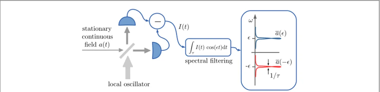
4.1. Single-mode homodyne spectrum and entangled spectral components

In homodyne detection the signalfield is mixed on a 50:50 beam splitter with a strong monochromatic field (the local oscillator) at the same frequency as the carrier signal. Thefields at the two output ports of the beam splitter are detected and the corresponding photocurrents are subtracted, resulting in a signal that contains information about afield quadrature [65] and that can be described by a photocurrent operator of the form (see appendixB)

= +

θ θ −θ

I( )( )t eia t( ) e ia t†( ), (27)

whereθ is the phase of the local oscillator. The power spectrum of the photocurrent contains information about the spectral components of the detectedfield, and in particular it quantifies the strength of the fluctuations at specific frequencies. We will refer to it as the homodyne spectrum, and it can be expressed as the autocorrelation function of thefiltered photocurrent, integrated over a long time τ, of the formJτ( , )θ φ ( , )ϵ t ∝ _τ

1

∫

_−τ ds

t t

ϵ_s+φ _Iθ _s

cos( ) ( )( ). In detail, the homodyne spectrum can be written as

ϵ = ϵ θ τ τ θ φ →∞ ( )( ) lim ⎡J( , )

(

,t

)

2 . (28) ⎣ ⎤⎦

We note that, for stationary processes, this quantity is independent of the phase of thefilter φ (see appendixB). However, this phase is relevant and can be useful when considering combinations offiltered photocurrents at different phases, which, as discussed hereafter, can be exploited to probe arbitrary superpositions of spectral modes. Moreover the same results for the power spectrum in equation (28) are obtained when, in thefiltered

photocurrentJτ( , )θ φ ( , )ϵ t , one uses an exponential oscillating function, as in thefilters of section2.1, in place of the sinusoidal function introduced earlier. The use of a sinusoidal function is, however, more convenient because, in this case, thefiltered photocurrent is a Hermitian operator, thereby making the relation between the photocurrent and thefield observables more transparent. Specifically the filtered photocurrent in the limit of longfiltering time can be expressed as the sum of two filtered quadrature operators for the two spectral modes at frequencies ϵ± (see appendixB):

ϵ ϵ ϵ ϵ = = + − θ φ τ τ θ φ θ φ θ φ →∞ + − J J t x x ( ) lim ( , ) 1 2 ( ) ( ) . (29) ( , ) ( , ) ( ) ( ) ⎡ ⎣ ⎤⎦

Similar to equation (19), this is a symmetric superposition of two quadratures, defined as in equation (18), corresponding to the two spectral components, which in this case arefiltered from the same field, and whose annihilation operators are

ϵ −ϵ

a( ) and a( ), (30)

as illustrated infigure1. The corresponding single-mode homodyne spectrum (where, single-mode, indicates that its results form the detection of a single continuousfield) is equal to equation (22) with ξ+=ξ−and θ++θ−= 2 , i.e.,θ ( )θ ( )ϵ =1+n+( )I + n−( )I +[m( ) 2 iI e θ+m( )I* e−2 iθ], where

ϵ ϵ ϵ ϵ

= ∓ ± = −

±

n( )I a†( ) (a ) , m( )I a( ) (a ) . (31)

Thus, the single-mode phase-optimized squeezing spectrum, which is experimentally accessible by tuning the phase of the local oscillator,S ( )( )I ϵ =minθ( )θ( )ϵ, is equal to equation (22) evaluated for the parameters in equation (31). When it is smaller than one, it indicates that the two sideband modesa (±ϵ) are entangled [37– 40]. Their logarithmic negativity, which as discussed in section3, is directly related to the squeezing spectrum in equation (23), could be measurable if one could construct afiltered photocurrent similar to equation (20), which is a non-symmetric superposition of the quadratures of the two modes. This photocurrent is, in fact, achievable by combining twofiltered photocurrents detected at appropriately tuned phases of the local oscillator θ and of thefilter φ. Specifically one should first detect the filtered photocurrentJ( , )θ φ( )ϵ _{for some value ofθ and φ and} then a second one,_J( ,θ φ′ ′)_{( )}ϵ_{, with the phases tuned to different valuesθ′andφ′. The two photocurrents are}

then summed, resulting in the total photocurrent ϵ ξ ξ ξ ϵ ξ ϵ = + + − ξ ξ θ θ θ θ + − + − + − + −

( )

+

( )

− J(_,, )( ) 1 x ( ) x ( ) , (32) 2 2 ⎡ ⎣⎢ ⎤⎦⎥

which we have appropriately normalized, and where

θ θ θ φ φ ξ θ θ φ φ = + ′ ± + ′ = − ′ ± − ′ ± ± ( ) 2 cos ( ) 2 . (33) ⎡ ⎣⎢ ⎤ ⎦⎥

We note that equation (32) has, indeed, the form of the composite quadrature defined in equation (20). The corresponding single-mode globally optimized squeezing spectrumSmin( )I ( )ϵ = θ ξ ξ ξ ϵ

θ θ ± ± + − + − ( ) J min , , ( ) , 2 ⎡ ⎣⎢ ⎤⎦⎥ is then

equal to equation (23) evaluated for the parameters in equation (31), and it can be measured by minimizing the homodyne spectrum over the phases of both the local oscillator and thefilter. In particular, although the tuning thefilter phases,φandφ′, can be, in principle, achieved by recording the photocurrent for a sufficiently long

Figure 1. Single-mode homodyne detection: a stationary continuousfield is detected by homodyne techniques and the resulting filtered photocurrent is a superposition of spectral components at opposite sideband frequencies±ϵ.

time and then post-processing the recorded signal, the phases of the local oscillator, θ andθ′, must be adjusted during repeated homodyne measurements.

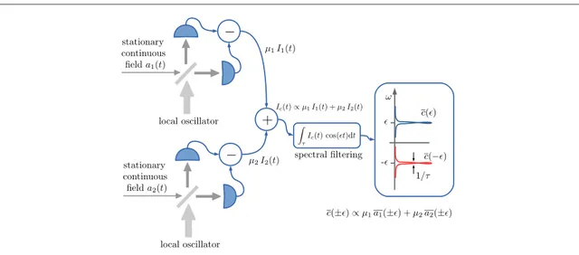
4.2. Two-mode homodyne spectrum and entangled spectral components

In the preceding section we saw that the single-mode homodyne spectrum, which is measurable from a single stationary continuousfield, provides information about the entanglement between two spectral components. Let us now study the two-mode squeezing spectrum obtained from the combination of two homodyne photocurrents which result from the measurement of two signalfieldsa t1( )and a t2( ), as depicted infigure2.

This strategy detects the correlations between four spectral components [68]. Specifically, we consider the situation in which the photocurrents corresponding to the two detectedfields,I1( )θ1( )t andI2( )θ2 ( )t , have the

form of equation (27) and are combined to construct the total photocurrent

μ μ μ μ = + + θ θ θ θ I_c( , )( )t 1 I ( )t I ( ) ,t (34) 1 2 2 2 1 1 ( ) 2 2( ) 1 2 ⎡⎣ 1 2 ⎤⎦

where we have introduced the scaling parametersμ₁andμ₂, which weight the two quadratures differently and hence provide a means to select arbitrary collective modes as discussed hereafter. These parameters are controllable experimentally, including the asymmetrical amplification and/or attenuation of the two photocurrents. The total photocurrent is then analyzed by frequency. As in the preceding case, thefiltered photocurrentJcθ θ ( )ϵ =limτ→∞ _τ

∫

_t−τ ds cos(ϵs+φ) Iθ θ ( )s

t

c

(1 2) 1 (1 2) _{can be decomposed into two spectral}

components at the frequencies ϵ± :

ϵ = ϵ + −ϵ θ θ+ − θ+ θ− J ( ) 1 x x 2 ( ) ( ) (35) ( ) ( ) c , ⎡⎣⎢ c c( ) ⎤⎦⎥ where θ±= θ θ ±φ + 2 1 2

, and where we have introduced the quadrature operators for the collective spectral modes defined as

ϵ = ϵ + −ϵ

θ θ −θ

xc( )( ) ei c( ) e ic†( ) (36)

with the collective annihilation and creation operators given by ϵ μ μ μ ϵ μ ϵ ϵ μ μ μ ϵ μ ϵ ± = + ± + ± ∓ = + ∓ + ∓ θ θ θ θ − − c a a c a a ( ) 1 e ( ) e ( ) , ( ) 1 e ( ) e ( ) , (37) 12 22 1 i 1 2 i 2 † 1 2 1 2 1 i 1† 2 i 2† c c c c ⎡⎣ ⎤⎦ ⎡ ⎣ ⎤⎦ where⎡c(±ϵ),c†(∓ϵ) =1

⎣ ⎤⎦ and θc=

(

θ1−θ2

)

2. Also in this case, thefiltered photocurrent is a composite quadrature of the from of equation (29). Thus, although it is constructed from the collective operators in equation (37), we can still apply the results of section3to conclude that the two-mode squeezing spectrum,

Figure 2. Two-mode homodyne detection: two stationary continuousfields are detected by homodyne techniques. The two photocurrents are summed and then analyzed by frequency. As in single-mode homodyne detection, the resulting totalfiltered photocurrent is a superposition of spectral modes at opposite sideband frequencies±ϵ. However, here each spectral mode [c (±ϵ)] can be decomposed as the superposition of two spectral components [a (1±ϵ)anda (2 ±ϵ)] at the same sideband frequency, each filtered from one of the two fields.

ϵ

S( )II ( ), obtained as the minimum over the phases θ±of the autocorrelation function of thefiltered current, has

the form of equation (22) but is evaluated with the parameters

ϵ ϵ μ μ μ μ θ μ μ ϵ ϵ μ μ μ μ μ μ = ∓ ± = + + + + = − = + + + + θ φ θ φ θ φ θ φ ± ± ± ± − ± + − + + − +

(

)

(

)

(

)

(

)

(

)

(

)

n c c v v v v m c c w w w w ( ) ( ) 2 cos 2 arg ( ) ( ) 1 e e e e , (38) c c ( ) † 1 2 (11) 2 2 (22) 1 2 (21) (21) 1 2 2 2 ( ) 1 2 2 2 1 2 i (11) 2 2 i (22) 1 2 i (12) i (21) 1 1 2 2 ⎡ ⎣ ⎤⎦ ⎡ ⎣⎢ ⎤⎦⎥ where ϵ ϵ ϵ ϵ = ∓ ± = − ± v a a w a a ( ) ( ) ( ) ( ) (39) jk j k jk j k ( ) † ( )

forj k, =1, 2. We remark thatS( )II ( )ϵ _{is found by minimizing the autocorrelation function of the photocurrent}

in equation (35) over θ±only, whereasθcand μjdefine the specific collective modes that are being probed and

arefixed. Therefore, in this case the conditionS( )II ( )ϵ <1_{indicates the entanglement of the collective modes} described by the operators in equation (37), each of which is a superpositions of the spectral components at the same sideband frequencies of the twofields. Moreover, as with the discussions of the single-mode homodyne spectrum, the corresponding logarithmic negativity can be, in turn, measured by summing twofiltered photocurrents, at different phases, of the form of equation (35) and then calculating the corresponding

autocorrelation function. The two-mode squeezing spectrumS_min( )II ( )ϵ is then found by minimizing this quantity over the phases of both the local oscillator and thefilter, and the result, in full similarity with the single-mode squeezing spectrum, is equal to equation (23) but now evaluated for the parameters in equation (38). 4.3. Detecting single spectral components with homodyne techniques

As discussed in the previous sections, it is possible to construct arbitrary superposition of spectral modes at opposite sideband frequencies by the superposition of two homodyne photocurrents. The corresponding total photocurrent is then given by equation (32). Similarly, when the phases in equation (33) are set to some values for which one of the two parameters ξ±is equal to zero, then a single spectral mode is detected.

When applied to two distinctfields, this approach would permit the investigation of the correlations between two distinct spectral modes each belonging to a differentfield. Let us, for example, assume that we repeat the pair of measurements resulting in the total photocurrent in equation (32) for two different

continuousfieldsa t1( )and a t2( ). The two resultant compositefiltered photocurrents are then, in general, given

by ξ ξ ϵ = ξ ϵ +ξ −ϵ ξ +ξ θ θ _{θ θ} + − + − + − + − _{+ −}

(

)

J , ( ) jx ( ) j x ( ) j j , , ( ) , ( ) 2, 2, j j j j _{j j} , , , , ⎡ _{, ,}

⎣ ⎤⎦ with the parameters defined as in

equation (33) and where here j = 1, 2 distinguishes the parameters corresponding to the measurements of the first and second fields respectively.

If, in each pair of measurements, we tune the phases of the local oscillators and of thefiltersto certain values for which θj−θ′ − −j ( 1) (j φj−φj′ =) πand θj−θ′ + −j ( 1) (j φj−φj′ ≠) πso that ξ−,1=ξ+,2=0, then

each composite photocurrent is proportional to a quadrature of a single spectral component corresponding respectively to the annihilation operators

ϵ −ϵ

a1( ) and a2( ). (40)

The two photocurrents are then summed together, after being multiplied by appropriately chosen scaling factors ζ±, so that the resulting total photocurrent is

ζ ζ ζ ϵ ζ ϵ = + + − θ θ + − + (+ ) − (− ) Jtot 1 x ( ) x ( ) , 2 2 1 2 ,1 ,2 ⎡ ⎣⎢ ⎤ ⎦⎥

where the single-mode quadraturesxj( )θ (±ϵ)are defined in equation (18). Thus, this protocol detects the combined quadrature defined in equation (20). The corresponding squeezing spectrum,S(III)( )ϵ_{, defined for} ζ+=ζ−, as the minimum of the autocorrelation function of the total photocurrent overθ+,1and θ−,2, is equal to

equation (22) and is obtained by appropriately tuning the phases of the local oscillator and thefilter during repeated homodyne measurements. Similarly,Smin(III)( )ϵ, defined as the minimum of the power spectrum of the total photocurrent overθ+,1, θ−,2and ζ±, is equal to equation (23). In particular, also in this case we can conclude

that this quantity is equivalent to the logarithmic negativity betweena ( )1 ϵ anda (2 −ϵ)when thefields are

Gaussian.

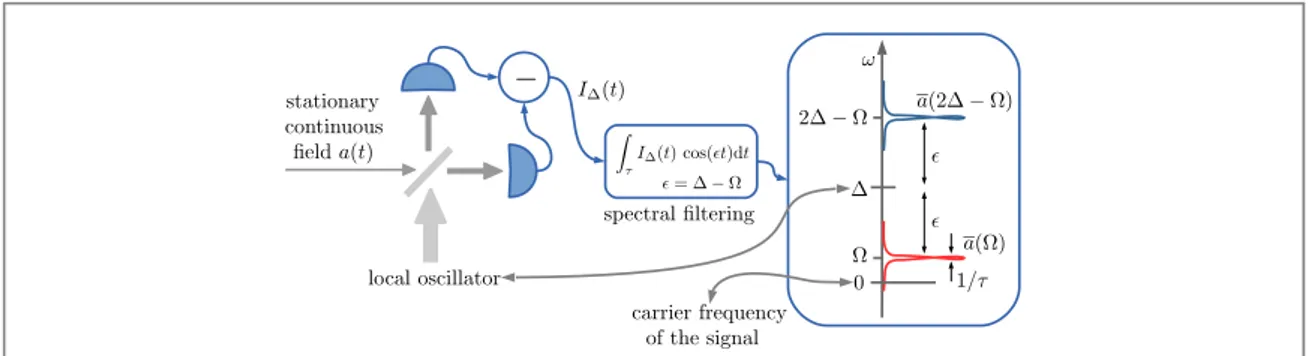
4.4. Two-mode heterodyne spectrum and entangled spectral components

An alternative strategy for probing single spectral modes and hence for measuring the squeezing spectrum, as well as the logarithmic negativity between two distinct spectral components of two distinctfields, as in section4.3, is based on heterodyne measurements.

In heterodyne techniques, the local oscillator is detuned from the carrier frequency of the signalfield by a quantity Δ=ωLO−ωL, and the corresponding operator for the photocurrent reads

= +

Δθ Δ θ −Δ −θ

I( )( )t e ei t ia t( ) e i te ia t†( ).

Hence, the correspondingfiltered photocurrent,JΔθ φ ( )ϵ = limτ→∞ _τ

∫

_−τ ds cos (ϵs+φ)IΔθ ( )s t

t

( , ) 1 ( )

, is the superposition of the quadratures for the spectral components at the frequenciesΔ±ϵ, namely

ϵ = Δ+ϵ + Δ−ϵ

Δθ φ θ φ+ θ φ−

J( , )( ) _⎣⎡x( )( ) x( )( )⎤_⎦ 2. Thus, whereas homodyne detection probes spectral components at opposite sideband frequencies, heterodyne techniques measure two components asymmetrically located with respect to the carrier frequency of the signalfield but symmetric with respect to the local oscillator frequency, which, in our description (where all frequencies are relative to the carrier signal), is equal toΔ (see figure3).

In particular heterodyne techniques can be used to detect a single spectral component, as discussed in the following. Say we want to detect the component at frequencyΩ; then we set the detuning Δ at a value much larger than the typical bandwidth of the signal Δ∣ ∣ ≫ Δsignal, which is the band of frequencies that are populated

by the signal photons. We also assume that the frequencyΩ is a relevant frequency for the field Ω∣ ∣ ⩽Δsignal.

Then the corresponding heterodyne photocurrent isfiltered at the frequency ϵ=Δ−Ωso that, as depicted in figure3, Δ ϵ

θ φ

J( , )( )is the superposition of thefield quadratures at the frequencies Ω and Δ2 −Ω:

Δ−Ω = Ω + Δ−Ω Δθ φ θ φ− θ φ+ J ( ) 1 x x 2 ( ) (2 ) . (41) ( , ) ⎡ ( ) ( ) ⎣ ⎤⎦

Since the signal covers a bandwidth much smaller thanΔ, the mode at Δ2 −Ωis basically in a vacuum and only the photons of the sidebandΩ are detected. However, in doing this the vacuum fluctuations of the empty component at Δ2 −Ωare added to the signal, resulting in higher noise.

This approach can be exploited to measure the correlations between two spectral modes belonging to two separatefields. Specifically the two-mode heterodyne spectrum is obtained when detecting two signals with two heterodyne measurements (withΔ≫Δsignal). The corresponding photocurrents arefiltered independently at

the frequenciesϵ1and ϵ2respectively, and then combined, with appropriately chosen scaling factorsξj, to

construct the totalfiltered photocurrent Δ ∝ξ Δ ϵ +ξ ϵ

θ φ Δ θ φ

(

)

(

)

J ,tot 1J ( ) J ( ) , 1 2 , 2

1 1 2 2 _{. If, in particular, we are interested} in the spectral components at frequencyΩ of the first field and at frequency−Ωof the second such that

Ω Δ

∣ ∣ ⩽ signal, we consider thefiltered photocurrents at the frequencies ϵ1= Δ−Ωand ϵ2=Δ+Ω. As in

equation (41) they are equal, respectively, to the superpositions of the two quadratures at frequenciesΩ and

Δ− Ω

2 of thefirst field and of the two quadratures at frequencies−Ωand Δ2 +Ωof the second. Correspondingly, the total photocurrent is given by

Figure 3. Single-mode heterodyne detection: a stationary continuousfield is detected by heterodyne techniques with the local oscillator at the frequencyΔ relative to the carrier frequency of the signal. The detected photocurrent is spectrally analyzed at the frequencyϵ=Δ−Ω. The resultingfiltered photocurrent is a superposition of spectral components at the frequencies Ω and

Δ−Ω

ξ Ω ξ Ω ξ ξ ξ Δ Ω ξ Δ Ω ξ ξ = + − + + − + + + Δ θ−φ θ−φ θ+φ θ+φ

(

)

(

)

(

)

(

)

J x ( ) x ( ) x x 2 (2 ) (2 ) 2 (42) tot , 1 1 2 2 12 22 1 1 2 2 12 22 1 1 2 2 1 1 2 2

where the quadrature operators for a single component are defined in equation (18). Its autocorrelation function is therefore given by Ω = + Δ ξ ξ θ−φ θ−φ

(

)

J 1 X 2 ( ) 1 2 (43) tot , 2 , , 2 1 2 1 1 2 2 ⎡⎣ ⎤⎦ ⎡_⎣⎢ ⎤_⎦⎥

where the term1

2on the right is due to the vacuumfluctuations of the spectral modes at Δ2 ± Ω, the collective

quadratureX_{ξ ξ}( , )θ θ_, ( )Ω

1 2

1 2 has the same form of the one defined in equation (_{20), and its autocorrelation function,} which is given in equation (22), quantifies the correlations between the modesa ( )1 Ω anda (2 −Ω).

Also in this case we define two kinds of optimized squeezing spectra. One is obtained by minimizing the autocorrelation function in equation (43), with ξ1=ξ2, only over the phases of the local oscillators

Ω = θ Δ

T( ) min J ,tot

2

j ⎡⎣ ⎤⎦ ;theotherisobtainedwhentheminimizationalsorunsoverthescalingparameters,

Ω = θ ξ Δ

Tmin( ) min , J ,tot

2

j j ⎡⎣ ⎤⎦ .Inbothcasestheycanbeexpressedintermsofthesqueezingspectraresulting

from the protocol described in section4.3as

Ω = Ω + Ω = Ω + T( ) S ( ) 1 T S 2 , ( ) ( ) 1 2 . (44) III III ( ) min min ( )

Thus, according to equation (26), in the Gaussian case,Tmin( )Ω measures the entanglement between the modes whose operators area ( )1 Ω anda (2 −Ω).

5. Application to ponderomotive squeezing in a two-sided cavity

Here we study ponderomotive squeezing [43–46] and the conditions under which the spectral components of thefield emitted by an optomechanical system are squeezed and entangled. Moreover we determine the squeezing spectra, and we identify the detectable spectral modes that exhibit maximum entanglement.

Ponderomotive squeezing refers to the squeezing of the output light resulting from the non-linear radiation-pressure interaction with a mechanical resonator inside an optical cavity. The response of a high-Q mechanical resonator to a resonance mode of a high-finesse optical cavity can be described as that of a Kerr medium, which imparts an intensity-dependent phase shift to the light. As a result thefield fluctuations can be reduced, and correspondingly, squeezed light is produced [43,44]. In detail, we investigate a Fabry–Perot cavity with a membrane in the middle [70]. A single optical mode is relevant in the system dynamics. It loses photons at rates

κ_jfrom the mirrors j = 1, 2 and is driven by a laser at a frequency detuned byδ from the relevant cavity resonance. Only one mechanical mode of the membrane at frequency ωminteracts significantly with the cavity field with a

linearized coupling strength g. The decay rate of the membrane isγ, and the number of thermal mechanical excitations nT. The corresponding linearized optomechanical dynamics are Gaussian [47,48] and are efficiently analyzed in terms of the standard input–output theory [69]. Here we describe the results for thefield emitted through the two cavity mirrors at the steady state of the system dynamics in the regime of optomechanical stability, referring the reader appendixCfor further details and derivations.

The photons lost through the two cavity mirrors are described by the outputfield operators aout1 ,a1out†, a out 2 , anda2out†. The corresponding power spectrum matrix, defined in equation (9), can be evaluated for the vector of

operatorsaout=

(

a1out,a2out,a1out†,a2out†

)

T, and the result is given by ω ω = ∣ ∣ + ∼  g     f ( ) 2 ( ) (45) out 2 2 out out

whereoutis a diagonal matrix whose diagonal elements are

(

2 ,κ1 2 ,κ2 2 ,κ1 2κ2

)

,is a matrix whose

only non zero elements are{ }1,3={ }3,4=1,

ω = δ ω − ω + γ− ω δ +

(

κ +κ − ω

)

f( ) 4g2 m m2 ( i )2 2 1 2 i , (46)

2

and the matrixis given in terms of the parameters α ω κ κ δ κ κ δ ω γ γ ω ω ω γ ω ω β ω κ κ γ κ κ δ ω γ ω ω ω ω = − + + − + + + + × + + + + − = + + + + ± + + + ∓ ω ±

(

)

(

)

(

)

(

)

(

)

(

)

(

)

(

)(

)

g n g n 4 i i 2 1 i 4 ( ) 2 1 2 (47) m T m m m m T m m 2 2 1 2 1 2 2 ₂ 2 2 2 2 2 2 2 2 1 2 1 2 2 _{2 2 2 2} ⎡ ⎣⎢ ⎤⎦⎥⎡⎣ ⎤ ⎦ ⎡ ⎣⎢ ⎤⎦⎥⎡⎣ ⎤⎦

(withα complex even function of ω, and β_±ωreal and positive) as

α α β β α α β β β β α α β β α α = ω ω ω ω ω ω ω ω − − − −  * * * * _{. (48)} ⎛ ⎝ ⎜ ⎜ ⎜ ⎜ ⎜ ⎞ ⎠ ⎟ ⎟ ⎟ ⎟ ⎟

This matrix contains all the information about the spectral properties of the outputfields and can be used to construct the correlation matrix for two spectral modes as in equation (15). In the following we will use this matrix and the results of sections3and4to study the corresponding entanglement properties.

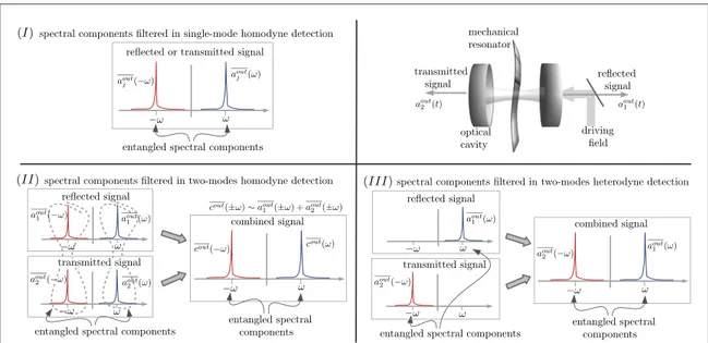
5.1. Homodyne and heterodyne spectra and entangled components of the emittedfield

In section4we described three different strategies for the experimental investigation of the spectral properties of stationary continuousfields, which are based on homodyne and heterodyne techinques. They probe different pairs of spectral modes given, respectively, by equations (30), (37), and (40). When applied to the investigation of the optomechanical system, these techniques allow the detection of the corresponding spectral components of the two outputfields ajout( )t , as depicted infigure4. In particular, using these techniques it is possible to study composite quadratures of these pairs of modes and their squeezing and entanglement properties. We have identified two different kinds of optimized squeezing spectra, corresponding to different experimental approaches for the measurement and the minimization of the homodyne photocurrentfluctuations.

Specifically, to probe symmetric superpositions of quadratures of the two modes it is sufficient to apply standard homodyne techniques; thus minimization is achieved by tuning the relative phase of the two quadratures, which is controlled experimentally by the phase of the local oscillator. We indicate this phase-optimized spectrum with the symbolS( )ℓ ( )ω _{, where the label ℓ = I II III, , is used to distinguish the three detection strategies (see}

figure4). At the same time, non-symmetric superpositions, with different weights of the two quadratures, can be probed by combining differentfiltered photocurrents detected with appropriately selected phases of both the filter and the local oscillator. The globally optimized squeezing spectrumS_min( )ℓ ( )ω is then obtained, minimizing the correspondingfluctuations over the phases of both the local oscillator and the filter.

Figure 4. Spectral components at the output of an optomechanical system that are probed with three different detection strategies and that are entangled, and squeezed, as a result of the optomechanical interaction.

In all cases the squeezing spectra_S( )ℓ_{( )}ω _and ℓ _ω

Smin( )( )are equal to equation (22) and (23), evaluated in each case for the specific parametersn±and m, which correspond to the detected spectral modes. Specifically,S ( )( )I ω

andSmin( )I ( )ω are obtained by the single-mode homodyne detection of a singlefield (either one of the two output

fields), as discussed in section4.1, and if applied to the output from thefirst mirror, then

ω ω

= ∓ ±

±

n( )I a₁out†( ) a₁out( ) andm( )I = a ( )ω a (−ω)

1out 1out . The second strategy is based on the

two-mode homodyne detection of the two outputfields (see section4.2), and the corresponding spectra,S( )II ( )ω _and ω

S_min( )II ( ), are evaluated forn±( )II = cjout†(∓ω)cjout(±ω) andm( )II = cjout( )ω cjout(−ω) , where the

operatorsc(out)(±ω)_{have the same form of equation (37), but in this case, they are constructed as the}

superpositions of the twofiltered output fieldsajout(±ω). Finally,S(III)( )ω andSmin(III)( )ω correspond to the

two-mode heterodyne detection of the two outputfields as discussed in section4.4. If it is applied to the spectral component at frequencyω of the first output and at−ωof the second thenS(III)( )ω _andS III _{( )ω}

min( ) are evaluated

forn±(III)= a1out†(∓ω) a2out(±ω) andm(III)= a1out( )ω a2out(−ω) . We note that these last two spectra

can also be retrieved by combining various homodyne photocurrents as discussed in section4.3. The power spectrum matrix in equation (45) can be used tofind

ω ω β β α ω ω β β α β β = + ∣ ∣ + − = + ∣ ∣ + − + − ℓ ℓ ω ℓ ω ℓ ℓ ℓ ℓ ω ℓ ω ℓ ℓ ℓ ω ℓ ω + − − + − + − − + −

(

+ − −

)

S g f q q q q S g f q q q q q q ( ) 1 4 ( ) 2 , ( ) 1 4 ( ) 4 ( ) 2 2 ( ) 2 ( ) 2 ( ) ( ) min( ) 2 2 ( ) 2 ( ) 2 ( ) ( ) 2 ( ) 2 ( ) 2 2 ⎡ ⎣⎢ ⎤⎦⎥ ⎡ ⎣ ⎢ ⎢ ⎤ ⎦ ⎥ ⎥ where κ μ κ μ κ μ μ κ κ = = = = + + = = θ θ + − + − − + − q q q q q q e e , , (49) I I II II III III ( ) ( ) 1 ( ) ( ) 1 i 1 2 i 2 1 2 2 2 ( ) 1 ( ) 2 c c

In the case of strategy II( ), the parameters μ_jandθc, in the expression forq_±( )II, determine the specific detected

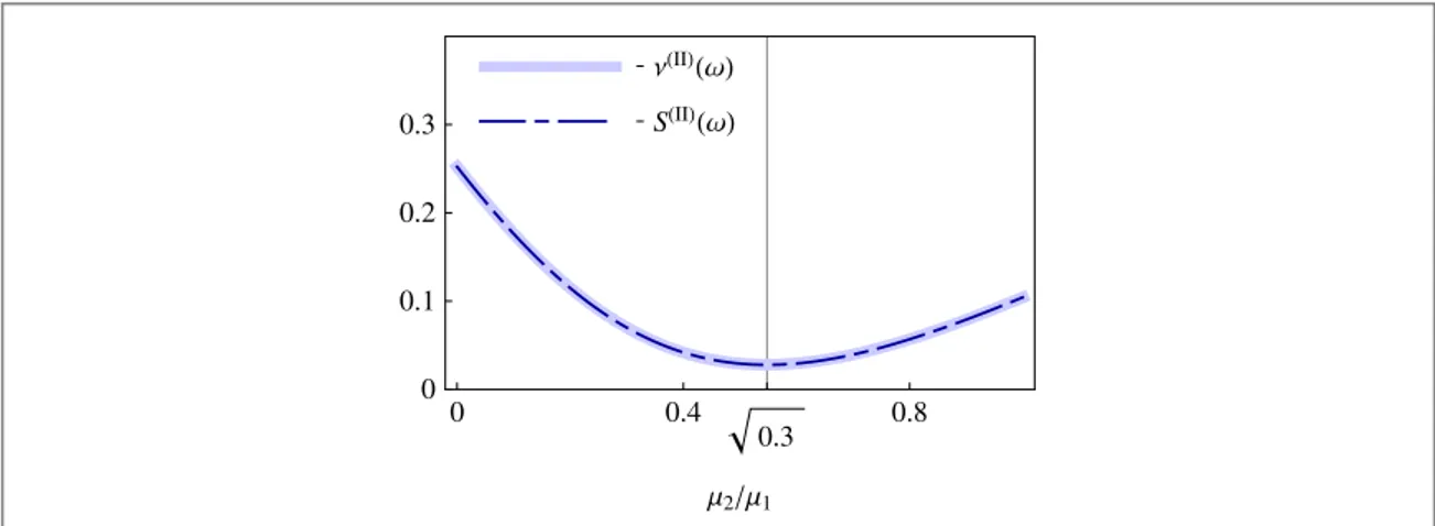
composite modes, which are defined as in equation (37). We observe that when

θc=0 and μ μ1 2 = κ κ1 2 (50)

thenq_±( )II =κ1+κ2; hence we can conclude thatSmin( )II ( )ω evaluated for a two-sided configuration with decay

ratesκ₁andκ₂is equal toSmin( )I ( )ω when it is evaluated for a single-sided cavity with the decay rate equal to the

sum of the decay ratesκ1+ κ2of the two-sided configuration. It indicates that the entanglement between ω

a1out( )anda1out(−ω), in a single-sided cavity, is redistributed among the four spectral componentsa1out(±ω)

anda₂out(±ω)in the case of a two-sided cavity. For this reason, the same amount of squeezing found in the case of a single-sided cavity, can be recovered when the information from the two decay channels of a two-sided cavity are properly combined. In particularq_±( )II is maximum for the parameters of equation (50) and

consequently the corresponding modes are the collective modes that are maximally squeezed (and entangled). We also note that according to equation (24) wefind that, in all cases, the pairs of spectral components are entangled (and squeezed), although possibly with different degrees of entanglement (and squeezing), when

β β_{ω −ω}< ∣ ∣α 2. (51)

Moreover we note that the logarithmic negativity between the pair of spectral components detected with each strategy is obtained by applying the definition in equation (25) to the parameter

ν( )ℓ( )ω =S ℓ ( ),ω min( )

which is equal to the minimum symplectic eigenvalue of the corresponding partially transposed covariance matrix.

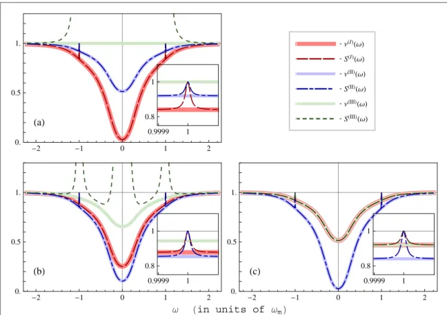
Infigure5we compare the results for the spectra evaluated for realistic parameters and corresponding to the three detection strategies, and hence to different pairs of spectral components. Each plot infigure5is evaluated for different values of the relative decay rateκ κ_{2 1}of the two mirrors, whereas the total decay rateκ1+κ2and all

the other parameters are keptfixed. In plot (a) we study a single-sided cavity with κ = 02 . In plot (b) the mirrors

are lossy and non-symmetric, andfinally in (c) the two mirrors are symmetric:κ1= κ2. When κ = 02 , in plot (a),