DIPARTIMENTO DI INGEGNERIA DELL’INFORMAZIONE, DELLE INFRASTRUTTURE E DELL’ENERGIA SOSTENIBILE (DIIES)
PHD IN INFORMATION ENGINEERING
S.S.D. ING-INF/02 XXX CICLO
SYNTHESIS OF INNOVATIVE
ELECTROMAGNETIC DEVICES VIA
INVERSE SCATTERING TECHNIQUES
CANDIDATE
Roberta Palmeri
ADVISOR
Prof. Tommaso Isernia
COORDINATOR
Prof. Claudio De Capua
Finito di stampare nel mese di Aprile 2018
Edizione
Quaderno N. 35
Collana Quaderni del Dottorato di Ricerca in Ingegneria dell’Informazione Curatore Prof. Claudio De Capua
ISBN 978-88-99352-23-3
Università degli Studi Mediterranea di Reggio Calabria Salita Melissari, Feo di Vito, Reggio Calabria
SYNTHESIS OF INNOVATIVE ELECTROMAGNETIC
DEVICES VIA INVERSE SCATTERING TECHNIQUES
The Teaching Staff of the PhD course in
INFORMATION ENGINEERING
consists of: Claudio DE CAPUA (coordinator)
Giovanni ANGIULLI Pier Luigi ANTONUCCI Giuseppe ARANITI Francesco BUCCAFURRI Rosario CARBONE Riccardo CAROTENUTO Salvatore COCO Francesco DELLA CORTE Fabio FILIANOTI Sofia GIUFFRE' Antonio IERA Tommaso ISERNIA Gianluca LAX Aime' LAY EKUAKILLE Giacomo MESSINA Antonella MOLINARO Andrea Francesco MORABITO Rosario MORELLO Fortunato PEZZIMENTI Sandro RAO Domenico ROSACI Giuseppe RUGGERI Francesco RUSSO Valerio SCORDAMAGLIA Domenico URSINO
insegnami la disciplina dandomi la pazienza e insegnami la scienza illuminandomi la mente. Sant’Agostino
At the end of my PhD studies, thanks are due to those people that have allowed the drafting of this thesis.
First of all, my absolute gratitude is to my advisor Prof. Tommaso Isernia, for having given me the possibility of join his research team and taught me how to scientifically face any problem, with unfailing support and dedication along the way. All the stimu-lating interactions I had with him have provided the keys to open the not yet explored parts of my mind.
During my PhD research activity, I was surrounded by precious coworkers. My great-est thanks to Dr. Martina Bevacqua. She has been a reference point for me from the beginning and working together, day by day, has made me grown a lot. I wish to express also my gratitude to Dr. Andrea Morabito for his kindness and support. Working with him, even if for a short time, it has been an honor. In covering all the LEMMA Research Group, my sincere thanks also go to my laboratory colleagues, Engs. Gennaro Bellizzi and Giada Battaglia, for the great time we spent together and for all the not-only professional discussions we had.
Moreover, I am thankful to Prof. Gino Sorbello and Dr. Loreto Di Donato. I will never forget my origin, so I would sincerely thank them for the time they dedicated me during the Bachelor and Master thesis, respectively, thus allowing me to explore the amazing world of electromagnetism.
I would like to thank also Dr. Lorenzo Crocco for the stimulating and fruitful dis-cussions and for his invaluable collaborations during these years, partially testified in this thesis.
But in life there is more than work. So, my sincere thanks also go to all the guys of Chemistry’s Laboratory, in particular to Fabiola for having shared both beautiful and hard moments during the PhD: they have been my family in Reggio Calabria. Last, but not least, a special thank goes to my family and Angela for their support and, in particular, to Giuseppe for always being close to me when I need and for pushing me to believe in myself.
Abstract
This Thesis deals with the synthesis of innovative microwave devices via in-verse scattering based theoretical tools and actual procedures. The electromagnetic scattering phenomenon occurs when the presence of an inhomogeneity in the space originates a perturbation of the field which is propagating. In the considered region of space, a new electromagnetic field occurs and such a total field is nothing but a superposition of the original one and the perturbation caused by the obstacle (or scatterer), which is called “scattered field”. The usual aim of an inverse scattering problem is to retrieve the location, the shape and the electromagnetic parameters of the scatterer by processing measurements of the scattered field. Several difficulties come into play in solving such a diagnosis problem, since the non linearity and the ill-posedness of the problem must be faced. Therefore, efficient solution strategies and regularization techniques have to be exploited to reach accurate and meaningful solutions.
Interestingly, the inverse scattering problem can be turned into a synthesis problem, provided the starting data is no longer a collection of measurements but rather some field specifications arising from design constraints. In the Thesis, some methodolo-gies already available in the inverse scattering community for diagnosis applica-tions are extended and modified for design purposes. Theoretical results include a new representation for non radiating sources and spectral analysis of some scat-tering approximations which are both of interest for design of invisibility devices. Methodological results include two new effective solution procedures for the general inverse scattering problem. Moreover, a well known inversion procedure is consid-erably modified and extended in order to include the synthesis of the excitations of some primary sources. Last, but not least, a new procedure is proposed for the synthesis of Artificial Materials based devices which outperforms a more intuitive homogenization based method. Finally, the developed approaches and procedures are validated through the synthesis of an optimal monopulse antennas as well as of new invisibility cloaks.
1 INTRODUCTION . . . 1
1.1 Inverse scattering problems: basics and difficulties . . . 1
1.2 The inverse scattering problem: basic equations . . . 3
1.2.1 Ill-posedness . . . 4
1.2.2 Non-linearity . . . 5
1.3 Rationale and contents of the thesis . . . 6
2 THEORETICAL AND METHODOLOGICAL ADVANCES IN INVERSE SCATTERING . . . 9
2.1 Some existing solution strategies . . . 9
2.1.1 Regularization techniques . . . 9
2.1.2 Methods to tackle the non-linearity . . . 10
2.2 The Compressive Sensing (CS) paradigm . . . 12
2.3 A spectral interpretation of approximated solution strategies. . . 14
2.3.1 The extended Born model . . . 14
2.3.2 Strong Permittivity Fluctuation model . . . 16
2.3.3 Some useful remarks for Born, CS-EB and SPF approximations 19 2.4 Two new inversion methods: the “DVE” and the “DIVE” approaches . 20 2.4.1 The virtual experiments framework and the “VELI” approximation . . . 20
2.4.2 The distorted virtual experiments (DVE) method . . . 23
Results: numerical data . . . 29
Results: experimental data . . . 32
2.4.3 The distorted iterated virtual experiments (DIVE) method . . . 36
Results: numerical data . . . 38
Results: experimental data . . . 43
2.5.1 A possible physical interpretation . . . 49
2.6 Concluding remarks . . . 51
3 SYNTHESIS OF VARIABLE MULTI-PURPOSE DIELECTRIC PROFILE ANTENNAS . . . 53
3.1 Introduction . . . 53
3.2 A new formulation of the Contrast Source Inversion (CSI) method: determining the amplitude of the primary sources . . . 54
3.3 Further modifications: enforcing desired properties on the unknown profile . . . 56
3.3.1 Exploiting inverse scattering and Compressive Sensing for design problems . . . 58
3.3.2 On the choice of the weighting parameters . . . 59
3.4 Assessment of the synthesis procedure . . . 59
3.4.1 Validating the proposed tool: (re)designing canonical lenses and beyond . . . 60
3.4.2 Design of antennas generating generic reconfigurable given patterns . . . 66
3.5 An Artificial Materials based solution . . . 71
3.5.1 Engineering the inclusions values: a new expansion for the contrast function . . . 72
3.5.2 Engineering the filling factor: a smart analytical tool . . . 73
3.5.3 Validating the developed tools . . . 75
3.5.4 A comparison with an alternative and more straightforward strategy . . . 78
3.6 Concluding remarks . . . 83
4 SYNTHESIS OF CLOAKING DEVICES . . . 85
4.1 Motivation and state of the art . . . 85
4.2 Invisibility within approximated models: spectral solutions . . . 87
4.3 ‘Full invisibility’ via inverse scattering methodologies . . . 91
4.4 Graded Artificial Material invisibility devices . . . 96
4.4.1 Figures of merit and bandwidth performances . . . 100
4.5 ‘Quasi-invisibility’ via inverse scattering methodologies . . . 101
4.6 Concluding remarks . . . 112
Appendix A . . . 119 Appendix B . . . 123 Appendix C . . . 125 Appendix D . . . 127 Appendix E . . . 131 References . . . 133 Publications . . . 145
2.1 Spectral interpretation of the CS-EBA (and also EBA). (a) Spectral coverage for the t-th experiment: the Ewald sphere. (b) Spectral
coverage for a set of experiments: the Ewald limiting sphere. . . 17 2.2 Pictorial view of the spectral meaning of the approximated inverse
scattering problem: (a) CS-EBA (and also EBA) (˜p = F [p]) and (b) SPFA(˜q = F [q]) . . . 19 2.3 DVE with numerical data: stratified scenario. (a) Real and (b)
imaginary part of the permittivity function of the reference scenario. (c) Real and (d) imaginary part of the permittivity function of the perturbed scenario: in the inner layer a ‘void’ is considered as
anomaly. (e) Real and (f) imaginary part of the actual unknown ˜". . 31 2.4 DVE with numerical data: stratified scenario. (a) Logarithmic plot
of the LSM map indicator when normalized to its maximum with superimposed the pivot points marked as stars for SNR=20 dB. (b) Real and (c) imaginary part of the retrieved perturbation "˜by means of DVE-TSVD. (d)-(f) are the same of (a)-(c) but for SNR=7 dB. (g) Real and (h) imaginary part of the retrieved perturbation
˜
"by means of DEBA-TSVD. (i)-(j) are the same of (g)-(h) but for DBA-TSVD. The black contour lines represent the geometry of the
actual scenario. . . 32 2.5 DVE with numerical data: stratified scenario. (a) Real and (b)
imaginary part of the retrieved perturbation ˜" in case of DVE with sparsity promoting regularization. (c)-(d) are the same of (a)-(b) but for DBA. . . 33
2.6 DVE with experimental data: FoamDielIntTM target at 3 GHz. (a) Reference profile. (b) Real and (c) imaginary part of the retrieved perturbation "˜by means of DBA-TSVD, superimposed to the reference permittivity function. (d) Logarithmic plot of the LSM map indicator when normalized to its maximum with superimposed the pivot points marked as stars. (e)-(f) are the same of (b)-(c) but for
DVE-TSVD. . . 35 2.7 DVE with experimental data: TwinFoamDielIntTM target at 4 GHz.
(a) Reference profile. (b) Real and (c) imaginary part of the retrieved perturbation "˜by means of DBA-TSVD, superimposed to the reference permittivity function. (d) Logarithmic plot of the LSM map indicator when normalized to its maximum with superimposed the pivot points marked as stars. (e)-(f) are the same of (b)-(c) but for
DVE-TSVD. . . 35 2.8 Flowchart of the DIVE scheme. . . 36 2.9 DIVE with numerical data: the ‘kite’ target. (a) Real and (b)
imaginary part of the actual contrast profile. . . 40 2.10 DIVE with numerical data: TSVD regularization. (a) Normalized
LSM indicator for the Initialization step with superimposed the pivot points marked as stars. (b) Real and (c) imaginary part of the obtained starting guess. (d) Normalized LSM indicator and pivot points for the first step of the iterative procedure (k = 1); (e) real and (f) imaginary part of the corresponding retrieved contrast profile at k = 1. (g) Normalized LSM indicator and pivot points for the last step of DIVE-TSVD scheme (k = 8); (h) real and (i) imaginary part of the final retrieved contrast function. (j) Real and (k) imaginary part of the final retrieved contrast profile by means of DBIM-TSVD after k = 3 iterations. . . 41
2.11 DIVE with numerical data: sparsity promoting regularization. (a) Normalized LSM indicator for the Initialization step with superimposed the pivot points marked as stars. (b) Real and (c) imaginary part of the obtained starting guess but with a sparsity promoting scheme. (d) Normalized LSM indicator and pivot points for the first step of the iterative procedure (k = 1); (e) real and (f) imaginary part of the corresponding retrieved contrast profile at k = 1. (g) Normalized LSM indicator and pivot points for the last step of DIVE-CS scheme (k = 7); (h) real and (i) imaginary part of the final retrieved contrast function. (j) Real and (k) imaginary part of the final retrieved contrast profile by means of DBIM with a sparsity promoting scheme and after k = 4 iterations. . . 42 2.12 DIVE with experimental data: Fresnel TwinDielTM target at 6 GHz.
(a) Reference profile. (b) Real and (c) imaginary part of the retrieved contrast function with DIVE-TSVD (during the iterative procedure NT = [117, 90, 148, 106, 91, 126, 115, 154, 122, 131, 142], for the initial
guess NT = 140); (d)-(e) are the same of (b)-(c) but for DIVE with
sparsity promoting regularization; (f)-(g) are the same of (d)-(e) but for a reduced number of processed data (see Table 2.3). . . 44 2.13 DIVE with experimental data: Fresnel FoamTwinDielIntTM
target at 4 GHz. (a) Reference profile. (b) Real and (c) imaginary part of the retrieved contrast function with DIVE-TSVD (during the iterative procedure
NT = [86, 73, 96, 72, 50, 74, 34, 67, 68, 83, 69, 48, 68, 91, 79, 89],
for the initial guess NT = 86); (d)-(e) are the same of (b)-(c) but for
DIVE with sparsity promoting regularization; (f)-(g) are the same of (d)-(e) but for a reduced number of processed data (see Table 2.4). . . . 45 2.14 DIVE with experimental data: Fresnel FoamDielIntTM target at 4
GHz. (a) Reference profile. (b) Real and (c) imaginary part of the retrieved contrast function with DIVE-TSVD (during the iterative procedure NT = [55, 36, 51, 40, 47, 35, 46, 51, 55], for the initial guess
NT = 47); (d)-(e) are the same of (b)-(c) but for DIVE with sparsity
promoting regularization; (f)-(g) are the same of (d)-(e) but for a
reduced number of processed data (see Table 2.5). . . 46 2.15 2D scenario for non-radiating currents. . . 48
2.16 Design of non radiating sources. (a) Synthesized coefficients and (b) comparison of the radiated field by the purely radiating Bessel
function (continuous line) and the synthesized NR source (dashed line). 50 3.1 Design of a dielectric antenna emulating the Luneburg lens. On the
left: permittivity distribution of the (a) canonical Luneburg lens and of the synthesized lens by exploiting (d) symmetry penalty term
s (ws = 1.148· 10 4, ⌧ = 1), (g) symmetry s and smooth ⇢2 (⇠ = 8.7 · 103, ⌧ = 0.6188 + j0.7146) penalty terms, (j) symmetry
sand smooth ⇢1 (⇠ = 10
8, ⌧ = 1) penalty terms. In the central
column: phase of the corresponding total field on a larger domain, in which the black line depicts the contour of the synthesized lens on the left. On the right: the radiated far fields from the lenses evaluated
starting from the aperture field. . . 62 3.2 Design of a dielectric antenna emulating the Luneburg lens. On
the top: discretized permittivity distribution of the synthesized one by exploiting (a) symmetry penalty term s (see Fig.3.1(d)), (b)
symmetry sand smooth ⇢2 penalty terms (see Fig.3.1(g)) and (c) symmetry sand smooth ⇢1 penalty terms (see Fig.3.1(j)). On the bottom: comparison of the radiated far fields between the continuous and the discretized lens for the three cases above. . . 63 3.3 Design of a dielectric antenna emulating the half Maxwell fish eye
(HMFE) lens. On the left: permittivity distribution of the synthesized lens by exploiting (a) symmetry penalty term s(ws= 10 6, ⌧ = 1),
(c) symmetry s and smooth ⇢2 (⇠ = 10
8,⌧ = 0.9135 + j0.0842)
penalty terms, (e) symmetry s and smooth ⇢1 (⇠ = 10
7, ⌧ = 1)
penalty terms. On the right: phase of the corresponding total field on a larger domain; the black line depicts the contour of the synthesized lens on the left. . . 65 3.4 Design of a dielectric antenna emulating the half Maxwell fish eye
(HMFE) lens. On the top: discretized permittivity distribution of the synthesized one by exploiting (a) symmetry penalty term s (see
Fig.3.3(d)), (b) symmetry s and smooth ⇢2 penalty terms (see Fig.3.3(g)) and (c) symmetry s and smooth ⇢1 penalty terms (see Fig.3.3(j)). On the bottom: comparison of the radiated far fields between the continuous and the discretized lens for the three cases
3.5 Synthesis of a ⌃/ reconfigurable pattern antenna: the reference scenario. Two sets of excitations are depicted: if the “black triangle” antenna is active, then a sum (⌃) pattern is radiated; if the “white triangle” antennas are active and excited with an opposite phase, then a difference ( ) pattern is radiated. . . 68 3.6 Synthesis of a ⌃/ reconfigurable pattern antenna. (a) Real part of
the permittivity function of the synthesized GRIN lens by inverse scattering and penalty terms sand f (ws= 2.5· 10 3, wf = 0.1,
Nc = 80⇥ 80). Far field (c) sum and (d) difference power patterns
radiated by the synthesized lens (dot-dashed blue lines). Continuous black and green lines represent the specified far field power patterns and the mask constraints, respectively. . . 69 3.7 Synthesis of a ⌃/ reconfigurable pattern antenna. (a) Real part of
the permittivity function of the synthesized GRIN lens by inverse scattering and penalty terms s, f and ⇢2 (ws = 2.5· 10
3,
wf = 0.1, ✏ =, Nc = 80⇥ 80). Far field (c) sum and (d) difference
power patterns radiated by the synthesized lens (dot-dashed blue lines). Continuous black and green lines represent the specified far
field power patterns and the mask constraints, respectively. . . 70 3.8 Graphic representation of the expansion’s basis in case of circularly
symmetric distribution. . . 73 3.9 Graphic representation of the expansion’s basis in case of circularly
symmetric and sparse distribution. . . 73 3.10 Magnitude of the scattering coefficient s0 (magenta lines), s1 (blue
lines) and s2 (black lines) for: (a) varying the contrast function at
fixed a = /20 (continuous line), a = /15 (dashed line) and a = /10 (dash-dotted line), (b) varying the radius of the cylinder at fixed
= 1(continuous line), = 2(dashed line) and = 3(dash-dotted line). . . 75 3.11 AM-based structure with a six-fold rotational symmetry. The
3.12 Synthesis of a ⌃/ reconfigurable pattern GAMs antenna, K = 11. (a) Real part of the permittivity function of the synthesized GAMR
lens by inverse scattering, expansion (3.11) and penalty term
s (wf =, Nc = 408⇥ 408) and (b) equivalent GAMF lens by
interchanging procedure ("r= 4.5, Nc = 1224⇥ 1224). Far field (c)
sum and (d) difference power patterns radiated by the synthesized lens (dot-dashed blue lines). Continuous black and green lines represent the specified far field power patterns and the mask constraints, respectively. 77 3.13 Synthesis of a ⌃/ reconfigurable pattern GAMs antenna, K = 9. (a)
Real part of the permittivity function of the synthesized GAMR lens
by inverse scattering, expansion (3.11) and penalty term s (wf =,
Nc = 408⇥ 408) and (b) equivalent GAMF lens by interchanging
procedure ("r = 4.5, Nc = 1224⇥ 1224). Far field (c) sum and (d)
difference power patterns radiated by the synthesized lens (dot-dashed blue lines). Continuous black and green lines represent the specified far field power patterns and the mask constraints, respectively. . . 78 3.14 Synthesis of a ⌃/ reconfigurable pattern GAMF antenna by
homogenization: case #1. (a) GAMF device derived from circularly
symmetric profile in Fig. 3.6(a) ("r= 4.5, Nc= 1224⇥ 1224) and the
corresponding far field (b) sum and (c) difference power patterns (dot red lines). Continuous black and green lines represent the specified far field power patterns and the mask constraints, respectively. . . 80 3.15 Synthesis of a ⌃/ reconfigurable pattern GAMF antenna by
homogenization: case #2. (a) GAMF device derived from circularly
symmetric profile in Fig. 3.7(a) ("r= 4.5, Nc= 1224⇥ 1224) and the
corresponding far field (b) sum and (c) difference power patterns (dot red lines). Continuous black and green lines represent the specified far field power patterns and the mask constraints, respectively. . . 81 4.1 Scattering Cancellation: a schematic interpretation of the transparency
phenomenon. . . 86 4.2 Transformation Optics: a schematic interpretation of the transparency
phenomenon. . . 87 4.3 Pictorial view of the spectral meaning of the approximated inverse
scattering problem for invisibility conditions: (a) BA (˜ = F [ ]), (b) CS-EBA (and also EBA) (˜p = F [p]) and (c) SPFA (˜q = F [q]). . . 88
4.4 Geometry of the problem for the synthesis of dielectric cloaking: ⌦ is the computational domain which includes an arbitrarily shaped scattering system made by the object to hidden ( 0 2 ⌃0) and the
cloaking region ( 2 ⌃), while is the observation region. . . 89 4.5 Schematic representation of the ‘alternate projections’ synthesis
approach. . . 90 4.6 Spectral invisibility via ‘alternate projections’ approach: a circular
object. Permittivity function of the (a) bare and (b) synthesized profile. Fourier transform of the (c) bare object ( ˜0) and of the (d)
synthesized cloaking system (˜); the white contour line represents the Ewald sphere with radius 2kb. Scattered field from the (e) bare and
(f) cloaking system on a larger domain with superimposed the contour line of the object. . . 91 4.7 Spectral invisibility via ‘alternate projections’ approach: three circular
objects. Permittivity function of the (a) bare and (b) synthesized profile. Fourier transform of the (c) bare object ( ˜0) and of the (d)
synthesized cloaking system (˜); the white contour line represents the Ewald sphere with radius 2kb. Scattered field from the (e) bare and
(f) cloaking system on a larger domain with superimposed the contour line of the object. . . 92 4.8 Full-aspect invisibility for cylindrical object. (a) Permittivity function
of the bare object and (b) real part of the total field for ✓t= 0 on a
larger domain with superimposed the contour of the bare object as a black line. . . 94 4.9 Full-aspect invisibility for cylindrical object. From top to bottom:
features of the GRIN cloaking system in case of circular symmetry (ws= 10 4, wf = 4· 10 4) and circular symmetry in conjunction
with smoothness (w⇢ = 10 12) penalty terms. (a)-(c) Synthesized
permittivity function and (b)-(d) real part of the total field on a larger domain, on which the contour of the cloaking system is superimposed as a black line. . . 95
4.10 Full-aspect invisibility for cylindrical object. From top to bottom: features of the GAMs cloaking system. On the left: synthesized permittivity function; on the right: real part of the total field on a larger domain with the contour of the system as a black line. Features and performances of (a)-(b) GAMR with K = 4, a = /15 and
d = /7(wf = 1.3· 10 4); GAMF for (c)-(d) "F = 5.5 and (e)-(f)
"F = 10. . . 98
4.11 Full-aspect invisibility for cylindrical object. From top to bottom: features of the GAMs cloaking system. On the left: synthesized permittivity function; on the right: real part of the total field on a larger domain with the contour of the system as a black line. Features and performances of (a)-(b) GAMR with K = 3, a = /11 and
d' /5 (wf = 9.7· 10 5); GAMF for (c)-(d) "F = 5and (e)-(f) "F = 9. 99
4.12 Full-aspect invisibility for cylindrical object. SCS calculated as a function of frequency for synthesized cloaks and comparison with the bare object.. . . 101 4.13 Quasi-invisibility for cylindrical object. (a) Permittivity function
of the bare object. (b) Geometry of the adopted measurement configuration: the observation region is a linear array at distance ro
from the origin of the reference system; the arrow on the left is the
impinging plane wave from ✓t= 180 . . . 103
4.14 Quasi-invisibility for cylindrical object. (a) Permittivity function of the synthesized cloak for a full invisibility requirement. (b) Magnitude and (c) phase of the radiated total field on . . . 103 4.15 Quasi-invisibility for cylindrical object. Features of the synthesized
cloaking system for: QI#1 on the left, QI#2 on the right. From top to bottom: (a)-(b) permittivity function; comparison of the performances in term of magnitude and phase of the (c)-(e) scattered and (d)-(f) total field on . The continuous blue line is the assigned design constraint, while the dotted green line and the marked blue
4.16 Quasi-invisibility for cylindrical object. Features of the synthesized cloaking system for QI#3. Synthesized permittivity function for (a) ↵ = 70 , (b) ↵ = 220 , (c) ↵ = 250 and (d) ↵ = 310 . Comparison of the performances in term of (e) magnitude and (f) phase of the total field on . The dotted green line is relative to the bare object, while the continuous and marked lines are relative to the assigned design
constraints and the achieved solutions, respectively. . . 106 4.17 Quasi-invisibility for cylindrical object. Features of the synthesized
cloaking system for joint QI#2-QI#3. Synthesized permittivity function for (a) ↵ = 70 , (b) ↵ = 220 , (c) ↵ = 250 and (d) ↵ = 310 . Comparison of the performances in term of (e) magnitude and (f) phase of the total field on . The dotted green line is relative to the bare object, while the continuous and marked lines are relative to the assigned design constraints and the achieved solutions, respectively. . . . 107 4.18 Quasi-invisibility for grid object. (a) Permittivity function of the bare
object. (b) Geometry of the adopted measurement configuration: the observation region is composed by four linear arrays at distance ro from the origin of the reference system; the arrows represent the
corresponding impinging plane waves from ✓t= 0 , 90 , 180 , 270 . . . 108
4.19 Quasi-invisibility for grid object. Features of the synthesized cloaking system for: QI#1 on the left, QI#2 on the right. From top to bottom: (a)-(b) permittivity function; comparison of the performances in term of magnitude and phase of the (c)-(e) scattered and (d)-(f) total field on . The continuous blue line is the assigned design constraint, while the dotted green line and the marked blue line are the fields from the bare and cloaked object, respectively. . . 109 4.20 Quasi-invisibility for grid object. Features of the synthesized cloaking
system for QI#3. Synthesized permittivity function for (a) ↵ = 10 , (b) ↵ = 70 , (c) ↵ = 210 and (d) ↵ = 350 . Comparison of the performances in term of (e) magnitude and (f) phase of the total field on . The dotted green line is relative to the bare object, while the continuous and marked lines are relative to the assigned design
4.21 Quasi-invisibility for grid object. Features of the synthesized cloaking system for joint QI#2-QI#3. Synthesized permittivity function for (a) ↵ = 10 , (b) ↵ = 70 , (c) ↵ = 210 and (d) ↵ = 350 . Comparison of the performances in term of (e) magnitude and (f) phase of the total field on . The dotted green line is relative to the bare object, while the continuous and marked lines are relative to the assigned
design constraints and the achieved solutions, respectively. . . 111 A.1 Graphical representation for Compressive Sensing understanding. (a)
A sparse vector s lies on a K-dimensional hyperplane aligned with the coordinate axes in RN and thus close to the axes. (b) Compressive
sensing recovery via `2 minimization does not find the correct sparse
solution s on the translated nullspace (green hyperplane) but rather the non-sparse vector ˆs. (c) With enough measurements, recovery via `1 minimization does find the correct sparse solution s. . . 121
2.1 DVE with numerical data: stratified scenario. Geometrical and dielectric properties (permittivity and conductivity) of the radially
layered scatterer from the outermost to the innermost layer . . . 29 2.2 DIVE for ‘kite’ target: details of the inversion procedure for different
analyzed approaches. . . 40 2.3 DIVE for Fresnel TwinDielTM target: details of the inversion procedure 43 2.4 DIVE for Fresnel FoamTwinDielIntTM target: details of the inversion
procedure . . . 45 2.5 DIVE for Fresnel FoamDielIntTM target: details of the inversion
procedure . . . 47 3.1 Synthesis of a ⌃/ reconfigurable pattern antenna: comparison of the
synthetic parameters for the far field patterns. . . 69 3.2 Synthesis of a ⌃/ reconfigurable pattern GAMs antenna: comparison
of the synthetic parameters for the far field patterns. . . 82 4.1 Figures of merit for the synthesized cloaking devices. . . 100
INTRODUCTION
1.1 Inverse scattering problems: basics and difficulties
The electromagnetic scattering [1–3] phenomenon occurs when the presence of an inhomogeneity in the space originates a perturbation of the field which is propagating, namely the incident field. In the considered region of space, a new electromagnetic field occurs and such a total field it is nothing but a superposition of the original one and the perturbation caused by the obstacle (or scatterer). This latter is called scattered field and it is generated by the target that interacts with the incident field during its propagation. As a matter of fact, from a physical point of view, the inhomogeneity (penetrable or metallic, magnetic or not) becomes a “source” for the scattered field.
The electromagnetic scattering can be faced by considering two types of problem, the forward scattering problem and the inverse scattering problem [4]. The former deals with the evaluation of the scattered field given the electromagnetic properties of the obstacle (and supposing obviously that the incident field is known). The latter copes with retrieving information on the scatterer by handling the measurements of the total (or scattered) field.
The direct and the inverse scattering problem are linked each other by a sort of duality. In fact, from a physical point of view, the cause of the phenomenon is the interaction between the incident field and the obstacles, while the corresponding effect is the scattered field which originates in the space. Notably, the role of the two problems can be inverted and the formulation of one implies the formulation of the other.
In the literature, the direct problem is the most investigated and a lot of work has been done in developing more and more efficient numerical methods and com-putational techniques. Conversely, the inverse scattering problem has deserved less attention, probably because of its much increased difficulty. In fact, it is very challeng-ing because of two different reasons, i.e., ill-posedness (accordchalleng-ing to the Hadamard’s definition [5]) and non-linearity. Obviously, a strong effort has been done by research
groups in developing effective solution strategies which counteract both ill-posedness and non-linearity in order to solve the inverse problem at best.
Finding solution methods that allow to accurately solve the problem is an im-portant task in a lot of application fields, thanks to the capability of microwaves of investigating non-accessible scenarios in a non-invasive way. Among all possible ap-plications involving in inverse scattering problems, it is worth to mention some of the most relevant area, which are:
• subsurface prospection including ground penetrating radar (GPR) and humani-tarian demining [6–9];
• non-destructive evaluation, as for example the search of small cracks inside struc-tures [10, 11];
• military and civil security surveillance, such as through-the-wall and intra-the-wall imaging [12, 13];
• medical imaging for tumor anomalies detection [14, 15].
In a classical inverse scattering experiment, a given region of the space is assumed to be illuminated by a set of incident fields radiated by some antennas located in the close-proximity or in the far field of the interested area. The interaction of the incident fields with the target in the region gives rise to a scattered field which is measured by a set of receiving antennas. These measured fields become the data of the inverse scattering problem and, by a proper processing of such data, the solution of the problem is obtained. In particular, depending on the problem at hand, one may attain information about position, dimension, shape, number of scatterers and so on. Anyway, the most general problem consists in the retrieval of both the geometrical and electromagnetic properties of the scenario at hand. Generally speaking, the more refined and detailed information about the scenario are required, the more difficult the solution of the inverse problem at hand.
For the reasons above, in the last three decades several models and approaches have been proposed to provide accurate qualitative (geometrical features) or quantita-tive (geometrical and electromagnetic features) solutions. However, several difficulties come into play which challenge the inverse scattering community towards the devel-opment of more and more convenient solution approaches.
First of all, the ill-posedness of the problem entails that only a finite number of parameters can be extracted from the scattered field data, as these latter have a finite essential dimension due to their band-limitedness property with respect to both incidence and observation variables [16–18].
Second, a crucial difficulty comes from the non-linearity of the problem. In fact, the non linear relationship among the physical parameters and the scattered fields represents a severe obstacle to the achievement of reliable solutions, as the so called “false solutions” [19] (i.e. retrieved profiles completely different from the actual one) may occur.
The mathematical formulation of the inverse scattering problem as well as a deeper insight into the ill-posedness and non linearity are given in the Sections which follow.
1.2 The inverse scattering problem: basic equations
By the sake of simplicity (most results of the thesis can be easily extended), let us consider the canonical bi-dimensional (2D) scalar scattering problem in a free space homogeneous background. Also, let us suppose to deal with non-magnetic dielectric scatterers whose cross-sections ⌃ are embedded in a region ⌦ ✓ R2. The
electromag-netic properties of the scatterer, at the angular frequency ! = 2⇡f, are described by the contrast function:
(r) = "˜r(r) ˜ "b 1 = "r(r) j r(r)/(!"0) "b j b/(!"0) 1 (1.1)
where r = (x, y) 2 ⌦, "0 is the permittivity of the free space, while "r, r, "b, b are
the relative permittivity and the electrical conductivity of the scatterer (subscript r) and the homogeneous background medium (subscript b), respectively.
Let suppose that an electric field, oriented along the z-axis, is radiated by a set of antennas located on a circumference and impinges on ⌦ from a given incident direction rt = (rr, ✓t) 2 . By assuming and omitting, for the sake of brevity, the
time harmonic factor exp(j!t), the equations ruling the inverse scattering problem, for the 2D TM scalar problem at hand, read [1–3]:
E(r, rt) = Ei(r, rt) + kb2 Z ⌦ g(r, r0) (r0)E(r0,r t)dr0 = Ei(r, rt) +Ai[ (r)E(r, rt)], r 2 ⌦, rt2 (1.2) Es(ro,rt) = k2b Z ⌦ g(ro,r0) (r0)E(r0,rt)dr0 =Ae[ (r)E(r, rt)], r 2 ⌦, ro,rt2 (1.3)
where Ei, Es and E are the incident, scattered and total field, respectively, ro =
(ro, ✓o)2 denotes the observation position, while Ae and Ai are a short notation
for the integral radiation operators, in which g(r, r0) = j/4H(2)
Green’s function of the background medium, H(2)
0 being the Hankel function of
zero-th order and second kind.
We refer to eq.(1.2) as state equation or, equivalently, electric field integral equation (EFIE), and to eq.(1.3) as data equation. In particular, the first one describes the total electric field inside the domain ⌦, while the second one represents the scattered electric field in the region outside the investigation domain.
The aim of an inverse scattering problem is to retrieve the contrast function (r) from the knowledge of the scattered field Es(ro,rt), which represents the data of the
problem, and the incident field Ei. As already mentioned, the problem is both non
linear and ill-posed. In fact, one can immediately observe that the total field inside the domain, which is obviously unknown as well, depends from the contrast function. In particular, in terms of the couple ( (r), E(r), r 2 ⌦), the inverse scattering problem is a bi-linear problem, i.e., the unknowns appear as a product between them: if we fix one of the two unknowns, the problem would become linear in the other one. The ill-posedness is instead related to the compactness of the radiation operator Ae[4].
More details on ill-posedness and non linearity properties, as well as on the corre-sponding impact on the problem solution, are given in the subsections which follow.
As a possible alternative, one can consider the currents induced inside the object as auxiliary unknowns instead of the total field. By defining the contrast source as W (r) = (r)E(r), the source type integral equation (STIE) formulation reads:
W (r, rt) = (r)Ei(r, rt) + k2b (r) Z ⌦ g(r, r0)W (r0,r t)dr0 = (r)Ei(r, rt) + (r)Ai[W (r, rt)], r 2 ⌦, rt2 (1.4)
while the data equation is turned into: Es(ro,rt) = kb2
Z
⌦
g(ro,r0)W (r0,rt)dr0=Ae[W (r, rt)], r 2 ⌦, ro,rt2
(1.5) where the new unknowns are the contrast function (r) and the contrast source W (r). Notably, the new data equation is now linear in the unknown W (r) [20,21]. At a first glance, it would seem that one can solve it, and then substitute the achieved value for W (r) in the state equation and solve it for (r). Unfortunately, this is not the case, as one cannot safely invert eq.(1.5) since it is a severely ill-posed problem.
1.2.1 Ill-posedness
A problem is defined ill-posed if it is not well-posed in the Hadamard’s sense [5]. In particular, a problem is well-posed if its solution (i) exists, (ii) is unique and
(iii) continuously depends on data. Otherwise, in the lack of one or more of these requirements, the problem is ill-posed.
Since for the inverse scattering problem at hand (involving non magnetic isotropic scatterers) the uniqueness of the solution is proved [22, 23] and it always exists, let us focus on the third requirement, which is herein missing. Such a circumstance leads to a ‘physical meaningless’ solution, since in presence of measurement uncertainties it may happen that to small variations occurring on data, do not correspond small variations in the solution which will be completely corrupted by noise.
From a mathematical point of view, in case of single-view experiment (i.e., a single illuminating incident field is used) the ill-posedness is due to the “compactness” of the scattering operator Ae[4] which relates the unknown target’s properties to scattered
fields. As a matter of fact, the inverse of a compact operator cannot be continuous, so that the continuity requirement from the Hadamard’s definition is violated. In particular, the generic unknown contrast belonging to an infinite dimensional space cannot be retrieved from the finite dimensional space of the collected information. In fact, whatever the kind of the scattering experiment, only a finite number of inde-pendent information can be reached, the so-called Degrees of Freedom (DoF) of the field [17,18]. Unfortunately, also in case of multi-view experiments (more illuminating incident waves are used) the problem remains ill-posed. This is due to the fact that also the incident fields belong to a compact set and, by paralleling the arguments for the single-view case, the scattering operator is still compact. Therefore, the number of independent equations is limited and a finite number of scattering experiments can be actually considered [18].
Note this latter circumstance (which is indeed undesired in recovery problems) is instead of interest in design problems, as one only needs to check (to enforce) a finite number of equations.
1.2.2 Non-linearity
The solution of the inverse scattering problem is usually pursued, in a least square sense, by minimizing a proper cost functional which takes into account both the data and the state equations. Due to the non-linearity of the underlying problem, this cost functional is a non-quadratic one, so that it may have many local minima which are “false solutions” of the problem [19]. In this kind of problem, a key role is played by the starting point of the minimization procedure, since if it does not belong to the attraction basin of the actual solution, a local minimum is reached and a solution far from the ground truth is obtained.
To get a better insight into the non-linearity, a physical interpretation of the issue could be sketched. When an incident wave interacts with objects in the space, a mutual scattering phenomenon occurs, i.e., higher order mutual interactions must be considered in the relationship between the scattered field and the objects.
By formally inverting the state equation (1.2) for the unknown E and substituting the result in eq.(1.3), the following expression is obtained:
Es=Ae[ (I Ai ) 1Ei] (1.6)
By exploiting the Neumann series for the term in round brackets, for kAi k < 1, the
final expression for the scattered field reads:
Es=Ae [IEi+Ai Ei+Ai Ai Ei+· · · ] (1.7)
where each addendum in brackets represents how gradually the mutual interactions increase, thus increasing the non linearity of the problem.
1.3 Rationale and contents of the thesis
The inverse scattering problem involves reconstruction of the property of a scatterer from the knowledge of its scattering data. During the years, the challenging nature of the problem has brought the inverse scattering community to develop more and more solution strategies for imaging problems. Needless to say, diagnosis methodolo-gies deserved interest especially in fields in which the human’s health and safety is of interest, like biomedical imaging for cancer detection and brastroke monitoring, in-vestigation of the reinforcement and condition of roads, bridges, and airport runways, the identification of structural integrity of buildings, demining, and so on.
On the contrary, in this thesis the inverse scattering problem is considered from the point of view of design problems. Saying it in other words, starting from a specification of a field pattern which takes the place of the scattering data, the corresponding scatterer (and eventually the amplitude of the primary sources, see the following) are synthesized. Note that such a change of the point of view allows to keep unaltered the problem’s formulation and hence the more general applicability of the theory.
Obviously, the intrinsic difficulties of the inverse scattering problem keep un-changed as well. However, since the imaging of an object is no longer of interest, the non-linearity issue is not a crucial point. In fact, whatever synthesized contrast function able to satisfy the (imposed) data of the problem is an admissible solution. This notwithstanding, a priori information as well as similar arguments of the usual
diagnosis problem can be exploited in order to proper conditioning the (still) ill-posed problem at hand and find the optimal solution.
The remainder of this thesis is composed by four chapters (including Conclusions) and five appendices (where mathematical details are deepened), and it is structured as follows.
In Chapter 2, after a brief summary of existing results, new theoretical and methodological contributions are presented for the inverse scattering problem. Coming to details, first (in the same spirit of the Born approximation) a Fourier based spectral analysis is derived for effective approximated solution strategies like the Extended Born, the Contrast Source Extended Born and the Strong Permittivity Fluctuation approximations. Beside their interest on the kind of profiles which can be actually retrieved or synthesized, the results also open the way to an accurate and reliable application of the recently introduced Compressive Sensing (CS) techniques (whose hypothesis do hold true).
Among the approximation-based solution strategies, the ‘virtual experiments’ (VE) framework has been recently introduced in literature as an effective approach for imaging non weak objects. Starting from its basic formulation, in the Chapter is pre-sented an extension of the VE to the case of inhomogeneous scenarios and hence the so-called distorted virtual experiments (DVE) approximation. Interestingly, VE and DVE can be jointly exploited into an iterative scheme to further enlarge the range of validity of the approximation itself. To this aim, the distorted iterated virtual ex-periments (DIVE) strategy is also derived and discussed. Beside the methodologies handling the non linearity property of the inverse scattering problem, an effective reg-ularization procedure based on CS is also proposed. In fact, CS has been developed, in the last years, as an effective tool for the solution of linear problems by exploiting a reduced number of data with respect to the unknowns; to this aim, this latter must be ‘sparse’ (i.e., with few elements different from zero) in a proper representation basis. Starting from this concept, the CS-based regularization is exploited for the solution of the approximated inverse scattering problem for both the DVE and DIVE strategies, thus allowing to reach more and more accurate solutions with respect to common regularization approaches in case of both numerical and experimental data.
Finally, by exploiting the well-known Devaney and Wolf’ theorems [24], a novel rep-resentation for the non-radiating currents is derived and assessed. Such a result is of interest both in the synthesis of invisibility devices as well as in antenna synthesis. In fact, the addition of a “non radiating” source to a given already synthesized source may simplify actual realization of the antenna.
In Chapter 3, the formulation of the inverse scattering problem as a design prob-lem is introduced. In this thesis, the probprob-lem is tackled in its full non linearity and the well-known Contrast Source Inversion (CSI) method is adopted. However, a proper reformulation of the CSI is proposed by considering the amplitudes of the incident fields as further unknowns, in order to deal with an accurate matching of the field specifications through possibly simpler devices. In this Chapter, the synthesis of di-electric profile antennas is pursued. Firstly, the synthesis of canonical lenses is attained as an assessment of the strategy. Then, antennas generating generic given patterns are looked for.
Although the reached devices show good performances and hence represent an inno-vative solution by per se, a further step toward actual manufacturing can be pursued by looking at artificial materials (AMs) based devices. As a first possibility, the syn-thesized gradient index (GRIN) dielectric profiles by means of the modified CSI is turned into a graded artificial materials (GAMs) device by exploiting homogenization theories. The second and more original strategy concerns instead to directly synthe-size a GAMs by using a proper representation basis for the unknown contrast function into the CSI functional.
Chapter 4 is then devoted to the synthesis of cloaks for invisibility scopes. In this thesis, volumetric cloaks are considered and the CSI method as well as several regu-larization techniques, already exploited for diagnosis problem, are herein adopted for the synthesis of cloaks with different characteristics. Among them, physical feasibility properties are the most interesting since they allow to deal with ‘natural’ material, thus avoiding metamaterials, which are the common solution for this kind of prob-lem. Moreover, the exploitation of the AMs-based solution introduced in Chapter 3 is also performed which make the GAMs cloaks the most effective solution. Finally, the spectral analysis introduced in Chapter 2 is herein turned into a possible way to design undetectable objects.
Conclusions and recommendations for further developments are finally drawn in Chapter 5.
THEORETICAL AND METHODOLOGICAL
ADVANCES IN INVERSE SCATTERING
2.1 Some existing solution strategies
In this Chapter, some tools for inverse scattering facilities are first reviewed in or-der to have a better insight of their possible usefulness in design problems. In this spirit, some canonical strategies are briefly recalled, by taking care on the basic lin-ear approximations as well as on their advanced variations which allow to extend the range of validity and taking into account some a priori information of the un-knowns of the problem. Along the same line, the recent paradigm of Compressive Sensing is briefly recalled and commented. Then, a spectral analysis of different use-ful approximations is introduced. As a second original contribution, two new solution strategies are proposed, both based on the new framework of ‘virtual experiments’, the distorted virtual experiments (DVE) and the distorted iterated virtual experiments (DIVE) approximations. Last, but not least, a new approach for the representation of non-radiating currents is proposed.
As already stressed, two not trivial issues make the inverse scattering phenomenon a complex problem, namely the ill-posedness and the non-linearity. In the following subsections, the main regularization techniques as well as strategies to counteract the non-linearity are briefly reviewed.
2.1.1 Regularization techniques
It was explained that the DoF of the scattered field constitute an upper bound for the significant data of the problem, for each scattering experiment [17, 18]. Therefore, a first possibility to increase such an amount of data is to perform additional scattering experiments. Several possibilities can be outlined: spatial diversity, frequency diversity or a combination of them. More in details, the spatial diversity aims at performing a number of experiments moving the illumination direction all around the investiga-tion space, in such a way that the collected data include the system’s response from
different points of view. Recently, new methods have been proposed in order to in-crease diversity [25, 26]. However, the above mentioned solutions cannot restore the well-posedness of the inverse scattering problem, since the number of independent information remains limited [18].
In order to restore the well-posedness of the problem, a huge amount of regularization techniques have been developed. The principle of the regularization methods is to use additional a priori information on the unknown in an explicit way in order to restore a unique solution compatible with the data.
As a first possibility, an energetic constraint can be added to the least square solu-tion in order to keep minimum the energy of the solusolu-tion; for instance, the Tikhonov regularization method [4, 27] aims to retrieve a minimum `2-norm energy.
However, some specific a priori information on the actual unknown (i.e., the contrast function) can be exploited and/or enforced. Just to mention a few:
i. enforcing a piecewise constant behavior on the contrast function [28–31]; ii. inducing physics bounds on the values of the unknown permittivity and
conduc-tivity functions;
iii. imposing a given finite alphabet of values for the permittivity function [32]; iv. imposing an upper bound on the dimensionality of the space where the unknown
function is looked for (‘regularization by projection’) [33–40].
The above listed techniques act on the contrast function ; however, similar concepts have been exploited on the auxiliary unknown W (r) [41].
Recently, the new paradigm of Compressive Sensing (CS) [42, 43] has been intro-duced in literature for linear problems. The key idea is that an ill-conditioned problem can be solved even if the number of data is lower than the number of unknowns, since the ‘sparsity’ or ‘compressibility’ of the unknown can act as regularizer of the problem. Essentials of the CS theory will be recalled with some detail in Section 2.2.
2.1.2 Methods to tackle the non-linearity
The adoption of linearizing approaches seems to be attractive to counteract the non-linearity of the inverse scattering problem, since the problem itself is simplified and different regularization techniques can be applied in a straightforward fashion. A lot of approximations have been proposed in literature during the years. Obviously, each approximation concerns a specific rationale and a situation of interest, that means they look for a particular class of objects by exploiting proper a priori information. On the other hand, they suffer from several limitations induced by the range of validity
of the introduced approximation.
The main linear approximations are listed below.
• The Born approximation (BA) [44] is valid for ‘weak scatterers’, i.e., when the internal characteristics of the scatterers are very close to those of the external medium and its dimension is very small as compared to the incoming wavelength. From a practical point of view, this assumption leads to substitute the unknown total field inside the operator’s kernel with the incident field, thus completely ne-glecting the presence of the object. Notably, by referring to eq.(1.7), the BA means to consider only the first term of the series, thus neglecting higher order mutual interactions. If the linearization is performed around a nominal scenario different from a homogeneous background, the underlying approximation is referred to as distorted Born approximation (DBA) [45].
• The Rytov approximation (RA) [46] holds for scatterers whose contrast function is smooth and low with respect to the background medium; moreover, no limits in the object’s dimension are considered since the total field is only approximated in its phase.
• The Kirchhoff or Physical optics approximation (PO) [46] is suitable for electri-cally large and strong scatterers; conversely with respect to the other methods, PO refers to the auxiliary unknown contrast source W (r), thus dealing with a kind of inverse source problem.
• The Strong permittivity fluctuation approximation (SPF) [47, 48] is instead valid for a set of different small scatterers and the problem is linearized and solved by means of an auxiliary unknown.
As an improvement with respect to the linearized methods, the quadratic approach [49,50] is also worth being mentioned. In this latter, a weak degree of non-linearity is introduced by adopting a second order approximation for the unknown-data mapping operator. As a consequence, the range of validity is wider compared to the BA, but also in this case the solution could be meaningfulness if the target’s parameters exceed the validity of the approximation.
Interestingly, by looking at different classes of scatterers, the BA has given rise to a number of different approximations. For instance, when non-weak scatterers are considered, the BA can be incorporated inside an iterative scheme. The arising so-lution approaches are the so-called Born iterative method (BIM) [51] and distorted Born iterative method (DBIM) [52]. At each iteration, the inverse problem is solved by applying the BA while the direct problem by updating the internal field (and the Green’s function in DBIM). Obviously, both approaches outperform the standard BA
but the final outcome and performances depend on the starting guess as well as on the range of validity of the intermediate linearizations. Other solution methods deriv-ing from BA are the Extended Born approximation (EBA) [53–56] and the Contrast Source Extended Born approximation (CS-EBA) [35, 57], which are viable in case of lossy host medium; in fact, by relying on the picked behavior of the Green’s function and the reduced intensity of mutual interactions in such a case, the inverse scatter-ing basic equations can be simplified and the arisscatter-ing linear problem is solved for an auxiliary unknown.
A more detailed explanation of some of the above approximations which includes a rigorous mathematical formulation is given in Section 2.3.
In order to overcome the limits due to the range of validity of each approximation, iterative optimization procedures which tackle the inverse problem in its full non-linearity have been proposed in literature. In this case, global optimization schemes should be adopted in order to avoid ‘false solutions’ [19], but they are not viable in case of large number of unknowns due to the exponential growth of the computational complexity. On the other hand, local iterative optimizations seem to be good candi-dates. Among these, the modified gradient method [34, 58, 59], the Contrast Source Inversion (CSI) method [20], the Contrast Source Extended Born model [21, 35] and the Subspace Optimization Method (SOM) [60] deserve to be mentioned.
It is worth to note that several strategies could be adopted in order to reduce the occurrence of ‘false solutions’. In particular, a good initial guess (e.g., reached by a pre-processing step) and/or some a priori information could constrain the minimiza-tion procedure in such a way that the searching space is reduced.
2.2 The Compressive Sensing (CS) paradigm
In the last years, the Compressive Sensing (CS) framework has emerged as an effective way to find meaningful solutions to undetermined systems describing linear models. As demonstrated by several contributions [61–63], the field of CS evolves from four decades. However, the idea of CS got a new life in 2004 when David Donoho, Em-manuel Candes, Justin Romberg, and Terence Tao gave important results regarding the mathematical foundation of CS [42, 64, 65].
The CS theory asserts that one can recover signals and images from far fewer samples or measurements than is possible using traditional methods, like for instance the Nyquist theory [65]. As it can be easily guessed, such a remarkable result is useful in very many scenarios in which limited number of samples can be actually collected [66].
As a matter of fact, part of the success of the CS paradigm (as witnessed by the very large number of papers being published on the subject) comes from statements such as ‘the possibility of overcoming the Nyquist criterion’ or to achieve ‘super-resolution’ in a number of recovery (and imaging) problems [65]. To make this possible, CS relies on two principles: sparsity, which pertains to the signals of interest, and incoherence, which pertains to the sensing modality. A signal is said sparse in a given representation basis, if it can be exactly represented by means of few non-zero elements; more precisely, the idea is that the ‘information rate’ of a continuous time signal may be much smaller than suggested by its bandwidth, or that a discrete-time signal depends on a number of DoF which is comparably much smaller than its (finite) length. As far as the incoherence property concerns, it is a concept related to the measurement process [65].
Provided the proper expansion is used in order to guarantee a sparse or compress-ible representation of the unknown function, CS theory guarantees that an accurate retrieval of the unknown is possible even for a number of data much lower than the overall number of basis coefficient, but sufficiently larger than the number of non-zero elements [65].
The above described peculiar features of CS has led to investigate such a recovery algorithm for inverse scattering problems, in particular for biomedical monitoring and non-invasive inspections [13, 67–74]. However, the adoption of the CS theory is not straightforward and the reason is twofold: first, the choice of a convenient representation basis for the specific problem at hand is not a trivial task; second, the intrinsic non-linear nature of the electromagnetic inverse scattering problem does not fulfill the theoretical results well developed and assessed for linear models.
For the reasons above, CS was firstly adopted for imaging of ‘point-like’ scatterers in conjunction with linear approximations such as the BA [69,75] or the DBIM [72,76]; later, the recovery of extended target has been exploited by considering the RA and the total variation (TV) approach [28]. Note that the CS tool allows to perform a ‘super resolution’ diagnosis by acting as a regularizer of the problem, but the validity of the mentioned approximations keeps still limited.
Recently, an effective imaging approach which exploits CS facilities for the solution of the inverse scattering problem in its full non-linearity has been proposed [77].
Interesting applicative and theoretical results have been also obtained in the field of antenna arrays diagnosis, both for linear [78–80] and non linear [81] models. In particular, for this latter case stimulating arguments about the incoherence property have been derived [81].
In this thesis, the CS paradigm will be exploited as a facilitator for design purposes. In fact, supposing a sparse unknown for the problem means that such a function is made by few elements different from zero. Correspondingly, the arising solution of the inverse scattering problem will be a more easily realizable device.
Applications of the CS paradigm in inverse scattering for design will be shown in the following Chapters, while for some simple understanding (and basics) the reader is deferred to Appendix A.
2.3 A spectral interpretation of approximated solution
strategies.
In this Section, an insight into the implication of the approximated approaches for the solution of the inverse scattering problem introduced in Sect.2.1 is given. In particular, by paralleling the results of the well-known BA [82], a Fourier analysis is proposed for the EBA, the CS-EBA and the SPF approximation (SPFA), which allows to gather a spectral interpretation of the strategy at hand.
Since the formulation for the EBA and CS-EBA is actually the same, a unique spectral analysis derivation will be tackled in the following.
2.3.1 The extended Born model
As is well known, the inverse scattering problem within the BA is viable and accurate when weak scatterers are looking for. As a matter of fact, the total field inside the in-vestigation domain is approximated with the background electric field, thus neglecting the effects that the scatterer induces into the field itself.
An improvement over the BA is achieved in the extended Born model [53], which results from an approximation arising from the peaked behavior of the Green’s func-tion in case of lossy background. Notably, in the same way as for the Born model, an extended Born series can be derived.
In this respect, let consider the STIE formulation for the state equation [21, 35]: W (r, rt) = (r)Ei(r, rt) + (r)
Z
⌦g(r r
0)W (r0,r
t)dr0 (2.1)
so that in the following it will refer to the contrast source extended Born (CS-EB) model.
By adding and subtracting W (r, rt)into the integral operator, the new state equation
W (r, rt) = (r)Ei(r, rt) + (r)W (r, rt) Z ⌦ g(r r0)dr0+ (r)Z ⌦ g(r r0) [W (r0,r t) W (r, rt)] dr0 = (r)Ei(r, rt) + (r)W (r, rt)f⌦(r) + (r)AiM OD[W (r, rt)] (2.2) where: f⌦(r) = Z ⌦g(r r 0)dr0 AiM OD[W (r, rt)] = Z ⌦ g(r r0) [W (r0,r t) W (r, rt)] dr0
By formally inverting twice eq.(2.2), one initially achieves:
W (r, rt) = p(r)Ei(r, rt) + p(r)AiM OD[W (r, rt)] (2.3)
in which:
p(r) = (r) I (r)f⌦(r)
and then, by defining I the identity operator:
W (r, rt) = (I p(r)AiM OD) 1p(r)Ei(r, rt) (2.4)
If kp(r)AiM ODk < 1, k·k being the `2-norm, a series expansion for the inverse operator
can be performed, thus obtaining the CS-EB series: W (r, rt) =
+1
X
n=0
(p(r)AiM OD)np(r)Ei(r, rt) (2.5)
Note that, as discussed is [21], the CS-EB series has been proved to be more rapidly converging that the Born series also in very many cases where the background is lossless.
From the singular nature of g(r r0)when r0=r one may expect that the dominant
contribution to the integral in eq.(2.2) is given by points close to r0 =r. Moreover,
the integrand of the second integral in eq.(2.2) is now integrable since the quantity in the square brackets vanish as r0! r where g is singular. As a consequence, in the
CS-EB approximation (CS-EBA) the second integral in eq.(2.2) is neglected since the first one plays a more significant role in deriving an approximation for the total field. Saying it in other words, the first term in the series (2.5) is the dominant one, so that the arising state equation for the CS-EBA reads:
W (r, rt) = p(r)Ei(r, rt) (2.6)
Finally, when the new approximation (2.6) is considered into the data equation, a linear inverse scattering problem in the unknown p(r) is achieved [21, 35]:
Es(ro,rt) =Ae[p(r)Ei(r, rt)] (2.7)
Note that, if the EFIE is considered rather than the STIE and the term (r)E(r) is added and subtracted into the integral operator, the same approximated model (2.6)-(2.7) can be derived for the extended Born approximation (EBA) [54, 55].
By paralleling the results of the BA, interesting arguments can be inferred when plane waves incident fields and far field observations are considered. In fact, under these assumptions, the expression for the scattered field reads:
Es(kt, ko) = C
Z
⌦
p(r0)e j(kt ko)·r0dr0 (2.8) in which ktand koare the vector of incidence and observation direction, respectively,
while C is a constant value arising from the asymptotic expansion of the radiation operator.
Interestingly, eq.(2.8) shows useful relationship with the Fourier transform F [·] of the auxiliary function. In fact, when this latter is evaluated, the following expression is gathered: F [p(r)] = ep(K) = Z ⌦ p(r0)e jK·r0 dr0 =Z ⌦ p(x, y)e j(kxx0+kyy0)dx0dy0 (2.9) The above equations (2.8)-(2.9) show that exists a relation between the scattered field and the spatial Fourier transform of the auxiliary variable p(r) encoding the original contrast function (r); in particular, Es(kt, ko) =p(ke t ko). In other words, Escan
be considered to be the restriction of the Fourier transform to the circle such that: kx= ktx+ kox
ky = kty+ koy
as long as k2
tx+ k2ty = !2"µ and kox2 + k2oy = !2"µ, " and µ being the permittivity
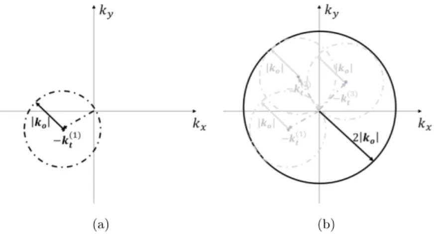
and permeability of the homogeneous free space, respectively. Therefore, the spatial frequencies set K maps, 8 experiment kt, the surface of a sphere of radius |ko| that
is centered at the point K = ktin the K space, see fig.2.1(a). This sphere is known
as Ewald sphere.
By considering a number of experiments |kt|, the final scattered field would be given
by ep(K) over the union of the surfaces of a number of Ewald spheres, namely over the bigger sphere with a radius of 2|ko| (the so-called Ewald limiting sphere), see
fig.2.1(b).
2.3.2 Strong Permittivity Fluctuation model
The SPF approximation (SPFA) has been introduced by Tsang and Kong [47] by exploiting the singularity of the Green’s function for the solution of the vectorial
(a) (b)
Fig. 2.1. Spectral interpretation of the CS-EBA (and also EBA). (a) Spectral coverage for the t-th experiment: the Ewald sphere. (b) Spectral coverage for a set of experiments: the Ewald limiting sphere.
problem of wave scattering by random medium in case of both small and large variance of the permittivity function. As a matter of fact, until then such a singular nature of the dyadic Green’s function was not taken into account thus applying and validating the random medium theory only in case of weak fluctuation.
Let us consider the state equation for the 2D vectorial case: E(r, rt) =Ei(r, rt) + Z ⌦ G(r, r0) k2 · E(r0,r t)dr0 =Ei(r, rt) + Ai⇥ k2· E(r, rt)⇤, r 2 ⌦ (2.10) in which: G(r, r0) =✓I 1 k2 brr ◆ g(r, r0)
is the dyadic Green’s function for homogeneous background medium, I is the 2D identity operator, g(r, r0) is the 2D scalar Green’s function and k2 = k2 k2
b, k
being the wavenumber of the random medium. The symbol (·) states for the inner product.
As it is known, the g(r, r0)function becomes singular when the observation point is
inside the source region and therefore the integral equation (2.10) results indetermi-nate. In order to overcome such a difficulty, by following the approach in [83], the singularity can be treated by means of the principal volume method, namely, by split-ting the integration domain into a small volume ⌦ surrounding the discontinuity and then let it approaches to zero, plus the remain ⌦ ⌦ part:
E(r, rt) =Ei(r, rt) + lim ⌦ !0 Z ⌦ ⌦ G(r, r0) k2 · E(r0,r t)dr0 + Z ⌦ G(r, r0) k2 · E(r0,r t)dr0 =Ei(r, rt) + lim ⌦ !0 Z ⌦ ⌦ G(r, r0) k2 · E(r0,rt)dr0 L· k2E(r, r t) k2 b (2.11) where L is a dyad depending on the shape of ⌦ . After simple manipulations, one achieves: ✓ I + k 2 k2 b L ◆ · E(r, rt) =Ei(r, rt) + P.V. Z ⌦ G(r, r0) k2 · E(r0,rt)dr0 (2.12)
where P.V.R⌦ stands for a shape dependent principal value integral. In particular, if
a cylinder is considered as volume ⌦ , L = I
2, while for a sphere L = I3 [83].
By defining [47, 48]: F(r, rt) = ✓ I + k 2 k2 b L ◆ · E(r, rt) = ⇣ I + L⌘· E(r, rt) q(r) = k2✓ I + k 2 k2 b L ◆ 1 =Iq(r) q(r) = k2 ✓ 1 + (r) 2 ◆ 1
the following state equation for the SPF model is derived: F(r, rt) =Ei(r, rt) + P.V. Z ⌦ G(r, r0)Iq(r0)· F(r0,r t)dr0 =Ei(r, rt) + AiSP F h Iq(r) · F(r, rt) i (2.13) As already done in Section 2.3.1, it is possible to formally invert (2.13):
F(r, rt) =
⇣
I AiSP F
h
Iq(r)i⌘ 1· Ei(r, rt) (2.14)
and define a series in case of AiSP F
h
Iq(r)i < 1, which reads: F(r, rt) = +1 X n=0 ⇣ AiSP F h Iq(r)i⌘n· Ei(r, rt) (2.15)
Finally, for AiSP F
h
Iq(r)i ⌧ 1 which surely holds true in case of the overall scattering system is constituted by many different (unconnected) small scatterers, the SPF approximation (SPFA) is obtained by considering only the first term of the summation (2.15):
![Fig. 2.2. Pictorial view of the spectral meaning of the approximated inverse scattering problem: (a) CS-EBA (and also EBA) (˜p = F [p]) and (b) SPFA(˜q = F [q]) .](https://thumb-eu.123doks.com/thumbv2/123dokorg/5027674.55819/47.918.356.700.478.664/pictorial-spectral-meaning-approximated-inverse-scattering-problem-spfa.webp)