Measurement of the
CP
violation parameter
A
Γ
in
D
0
→ K
+
K
−
and
D
0
→ π
+
π
−
decays
Classe di Scienze Matematiche e Naturali Corso di Perfezionamento in Fisica
PhD Thesis
Pietro Marino
Advisor: Dr. Michael J. Morello
Abstract
Time-dependent CP asymmetries in the decay rates of the singly Cabibbo-suppressed decays D0→ K+K−and D0→ π+π−are measured in pp collision data at centre-of-mass energies of 7 and 8TeV collected by the LHCb detector during LHC Run I, corresponding to an integrated luminosity of 3 fb−1. The strong-interaction decay D∗+→ D0π+is used to infer the flavour of the D0mesons at production. The asymmetries in effective decay widths between D0and D0 decays, sensitive to indirect CP violation, are measured to be
AΓ(D0→ K+K−) = (−0.30 ± 0.32 ± 0.10) × 10−3, AΓ(D0→ π+π−) = ( 0.46 ± 0.58 ± 0.12) × 10−3,
where the first quoted uncertainty is statistical, and the second systematic. These measure-ments show no evidence of CP violation and improve on the precision of the previous best measurements by nearly a factor of two.
Contents
Abstract i
Contents iii
Introduction 1
1 Theory and motivations 5
1.1 The Standard Model of Particle Physics . . . 5
1.2 The CKM matrix . . . 9
1.3 Unitary triangles . . . 11
1.3.1 Charm triangle parameters . . . 12
1.4 Neutral meson mixing . . . 13
1.4.1 Time evolution of flavour eigenstates . . . 14
1.4.2 Mixing phenomenology . . . 17
1.5 C P violation formalism . . . . 19
1.5.1 C P violation in the decay . . . . 20
1.5.2 C P violation in the mixing . . . . 21
1.5.3 C P violation in the interference . . . . 21
1.6 D0time-dependent decay rates to C P-eigenstates . . . . 21
1.6.1 Effective decay widths . . . 22
1.7 Time dependent C P asymmetry . . . . 23
1.8 AΓand yC Pobservables . . . 24
1.8.1 Experimental approximations . . . 25
2 Measurement overview and current experimental status 29 2.1 D0→ h+h−decays and flavour tag . . . 29
2.2 From the theory to the AΓmeasurement . . . 30
2.2.1 Raw CP asymmetry . . . . 32
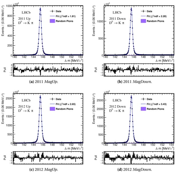
2.3 Control channel: D0→ K−π+decays . . . . 33
2.4 Physical background to AΓ: secondary decays . . . 33
2.5 Current experimental status . . . 34
2.5.1 Experiments at e+e−colliders . . . . 35
3 Experimental apparatus 39 3.1 LHC . . . 39 3.1.1 Luminosity at LHCb . . . 40 3.2 LHCb Experiment . . . 41 3.2.1 Coordinate system . . . 44 3.2.2 Magnet . . . 44 3.2.3 Vertex Locator . . . 45 3.2.4 Tracker Turicensis . . . 47 3.2.5 T-stations . . . 47 3.2.6 Cherenkov detectors . . . 49 3.2.7 Calorimeter system . . . 50 3.2.8 Muon detectors . . . 51 3.2.9 Trigger . . . 52 3.2.10 Data processing . . . 54 3.2.11 Event reconstruction . . . 54
4 Reconstruction and selection ofD0mesons 59 4.1 D∗+→ D0(→ h+h−)π+decays at LHCb . . . . 59
4.2 Trigger system . . . 61
4.3 Preselection . . . 63
4.4 Offline Selection . . . 64
4.5 Multiple candidates . . . 69
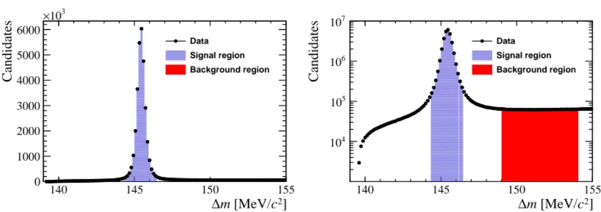
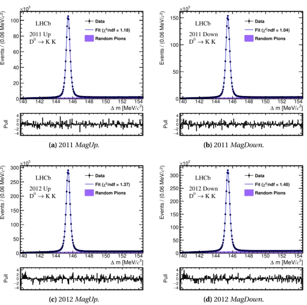
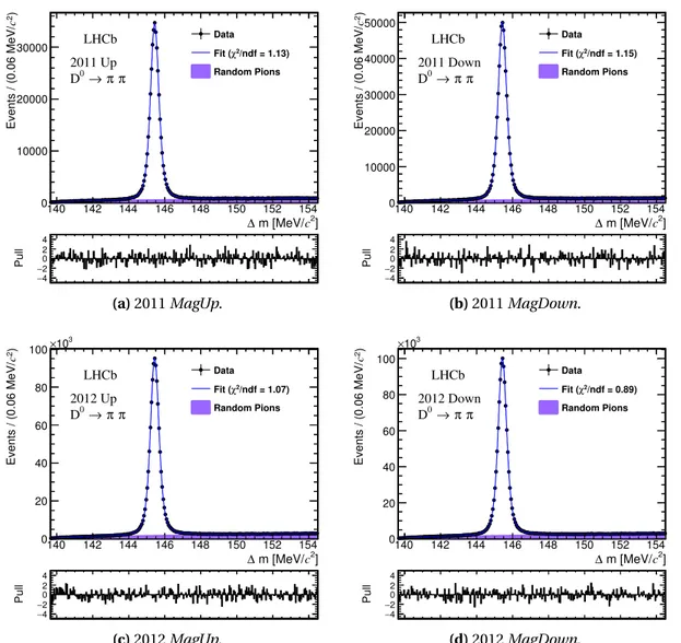
4.6 Sideband subtraction and ∆m fit . . . . 69
4.7 Charge-randomised sample . . . 74
5 Detector-induced time-dependent charge asymmetries 75 5.1 Introduction . . . 75
5.2 Control channel pseudo-AΓ . . . 76
5.3 Time-dependent instrumental effects . . . 78
5.4 Symmetrisation procedure . . . 79
5.4.1 Effects of the correction . . . 84
5.4.2 Could the symmetrisation procedure bias the value of AΓ? . . . 85
5.4.3 Indirect generation of time-dependent asymmetries . . . 87
5.5 Robustness cross-checks . . . 89
6 The extraction ofAΓparameter 93 6.1 Analysis strategy . . . 93
6.2 Results . . . 94
6.3 Robustness cross-checks . . . 98
6.4 Analysis validation . . . 103
7 Systematic uncertainty on secondary decays 105 7.1 Introduction . . . 105
Contents
7.2 Model of secondary decays . . . 106
7.3 Evaluation of secondary fraction fsec . . . 108
7.4 Evaluation of Asec . . . 109
7.5 Systematic uncertainty and robustness checks . . . 111
8 Robusteness checks and systematic uncertanties 115 8.1 Discretisation of the correction procedure . . . 115
8.2 Subtraction of random pion background . . . 116
8.3 Peaking backgrounds . . . 118
8.4 L0 trigger effects . . . 120
8.5 Multiple candidates . . . 121
8.6 Decay time resolution . . . 121
8.7 Summary . . . 122
9 Results and conclusion 123 9.1 Final results . . . 123
9.1.1 Combination . . . 123
9.2 AΓimplications on charm CP violating parameters . . . . 125
9.3 Future perspectives . . . 126 9.4 Conclusions . . . 128 A D0→ K∓π±decay rates 129 A.1 Pseudo-AΓ . . . 130 B Mathematical formalism 133 B.1 Tagged D0→ h+h−events . . . . 133 B.2 Tagged D0→ K−π+events . . . . 135 C AΓplots Legend 137 D Proper decay time bins 139 E Reweighing details 143 E.1 Symmetric reweigh . . . 143
E.2 Reweigh procedure of the asymmetry . . . 144
E.3 Reweighing weights . . . 147
E.4 Statistical degradation . . . 150
F Studies of assumptions about secondary decays model 153
Introduction
Over the course of the last 30 years, the Standard Model (SM) of elementary particles and their interactions has been extensively tested by experiments, establishing it as an extremely predictive and accurate description of Nature. Nevertheless, open questions and weaknesses remain, which suggest the need for a more fundamental theory. SM is not able to account for the cosmological observed baryonic-asymmetry and for the presence of Dark Matter in our Universe; the very low value of the Higgs mass is explained only through an “unnatural” fine-tuning cancellation between the radiative corrections and the bare mass; many parameters are necessary to account, in one-to-one correspondence, for the observed masses and mixings of quarks and leptons; lastly the gravity is not yet satisfactorily included in the model. The search for experimental deviations from SM predictions, pointing the way to a different, more fundamental theory, is therefore the primary goal of the High Energy Physics community. From the experimental point of view this quest is conducted at two frontiers: (i) the “high energy frontier”, which directly searches for hints of physics beyond the Standard Model (BSM) increasing the energy scale, and (ii) the “high intensity frontier” looking for inconsistencies between experimental measurements and theory predictions. At the first frontier, where ATLAS and CMS experiments are today the major players, New Physics (NP) is directly probed producing particles at more and more high energy and the main limitation comes only from the maximum achievable energy. The second frontier, instead, is based on performing more and more precise measurements, of known processes, by looking for discrepancies from SM predictions, and allows the indirect exploration of energies even higher than those accessible through direct searches. Of particular importance are processes having a low level of “SM noise”, or in other words, processes suppressed within the SM or where the SM contribution is known with high precision. This is the domain of Heavy Flavour Physics, currently probed mainly by the LHCb, Belle II and BES III experiments, where the non-invariance of fundamen-tal interactions under the combined symmetry transformations of charge conjugation and parity inversion (CP violation) plays a key role.
CP violation is described within the Standard Model through the Cabibbo-Kobayashi-Maskawa (CKM) mechanism [1,2] by the presence of a single complex phase in the unitary three-generation quark-mixing matrix. All direct measurements of elementary particle phenomena to date support the CKM phase, within the current theoretical and experimental uncertainties, being the dominant source of CP violation observed in quark transitions. However, widely
accepted theoretical arguments and cosmological observations, as mentioned above, suggest that the SM might be a lower-energy approximation of more generally valid theories which are likely to possess a different CP structure and therefore should manifest themselves as deviations from the CKM scheme.
The charm sector is today a particularly good candidate to probe possible deviations from the theory, since the expected CP violation in the SM does not exceed O(10−2) [3–6], and a sizeable CP asymmetry would stand up as a possible manifestation of NP. The system of D neutral mesons is the only one in which the oscillation of an up-type quark can occur, and it is the only one sensitive to possible contributions to CP violation of up-type quark through mixing loops. In fact, top quarks decay before hadronizing [7], and particles composed by u and u, like π0and η, are their own antiparticle, thus they are not able to oscillate as a matter of principle. Only very recently experiments have been able to collect and analyse huge samples of charm decays O(107) approaching for the first time the upper boundaries of the range of SM predictions, and possible NP contributions may completely have been missed by experimental searches so far. Therefore, the charm sector is a unique portal for obtaining an access to a new flavour dynamics. In addition, the complementarity to B and K meson systems, that have been much more deeply experimentally studied in the past decades, makes the exploration of the charm sector important by itself, for improving the current knowledge of heavy flavour dynamics within the SM. CP violation has not yet been observed in the charm sector, and only recently the slow mixing rate of the D0–D0flavour oscillations has been established [8], providing definitely a full range of probes for mixing and CP violation.
Except for a limited series of relevant experimental observables, hadronic uncertainties may greatly impact/limit the sensitivity of charm decays in probing new effects [9]. However, the increasing in precision of experimental measurements, together with the foreseen reduction on the uncertainties of several QCD parameters, should lead to a significant shrinkage of the theoretical uncertainties in the charm sector, and in many other flavour areas, allowing a powerful test of SM predictions in the next and far future. Anyway, it is worth to point out that an extensive study of the charm decays, and in general of the heavy flavour physics, at much higher precision than today is fundamental to over-constrain the theory parameters, and in particular the CKM scheme, that is a crucial ingredient for the SM and for any new exotic theory, which must include the flavour structure.
Examples of experimentally clean channels allowing the study of the CP violation in the charm system are the neutral singly-Cabibbo-suppressed decays into CP-eigenstates, such as D0→ f , where f = K+K−and f = π+π−, which are now available in large numbers from hadron collisions. A golden observable sensitive to possible effects of CP violation is the AΓ parameter, defined as the asymmetry of the effective decay widths ˆΓ, i.e. the inverse of the effective lifetimes, of the D0and D0decays
AΓ≡
ˆΓ(D0→ f ) − ˆΓ(D0→ f )
Introduction
Due to the slow mixing rate (x = ∆M/Γ < 1%, y = ∆Γ/2Γ < 1%) [10], and in the limit of negligible CP violation in the mixing, it can be found that AΓ≈ −x sinφDand its measure-ment translates into a constraint of the mixing phase φD, if the value of the x parameter is determined elsewhere. This also implies that AΓ≤ |x| < 5 × 10⁻³, and therefore, from an exper-imental point of view, it is particularly relevant to increase as much as possible the precision on the measurement of such an observable, well beyond the level of 10−3.
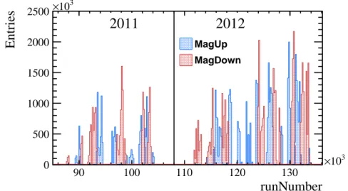
This thesis presents the world best measurement of the CP violation AΓparameter with pp collision data collected by LHCb in Run I, corresponding to an integrated luminosity of 3 fb−1, with 1 fb−1collected during 2011 at a centre-of-mass energy of 7TeV and the remaining 2 fb−1 collected during 2012 at a centre-of-mass energy of 8TeV. The achieved uncertainty on AΓ is for the first time approaching a level of about 10−4and the final result fully dominates the world average being the most precise measurement of CP violation ever of the LHCb experiment. Beyond the intrinsic importance of searching for first hints of CP violation in the charm sector at an unprecedented level of precision, the experimental methodologies developed in the thesis demonstrate that LHCb will be able to perform this measurement even at higher precision by fully exploiting the larger data samples that will be available in the future LHC Runs (LHCb-Upgrade and Future Upgrades).
I personally presented the results described in this thesis, for the first time, on behalf the LHCb Collaboration, at the VIII International Workshop on Charm Physics (CHARM 2016), 5-9 September 2016 - Bologna (Italy) [11] and a public LHCb document [12] was released at that time to accompany them. They have been submitted by the LHCb Collaboration to Physical Review Letters journal [13] on February 2017, and recently they have been accepted for publication.
The thesis is structured as follows. Chapter1introduces the theoretical framework of the CP violation within the Standard Model and the formal definition of the AΓobservable. Chapter2 describes the main experimental techniques to measure AΓalong with the current experimen-tal status. Chapter3briefly outlines the experimental apparatus, with particular attention on the LHCb sub-detectors relevant for the measurement described in the thesis. The candidates reconstruction and selection are reported in chapter4, together with the signal extraction. Chapter5is devoted to the description of the subtle, and therefore very dangerous, time-dependent detection charge asymmetries present in the reconstructed data sample, and to the innovative correction, specifically developed in this thesis, to keep such effects under control at a level of 10−4. Afterwards, chapter6reports the measurement of the AΓobservable in D0→ K+K−and D0→ π+π−decay modes. The following two chapters7and8are dedicated to the estimation of systematic uncertainties. The dominant systematic uncertainty is separately discussed in chapter7, where a new approach, which uses both analytical and data-driven information, has been successfully devised. Finally, chapter9presents the final results and a discussion of their impact on the current experimental panorama.
1
Theory and motivations
A brief review1of the Standard Model of particle physics is given in this chapter, with a partic-ular attention to the Cabibbo-Kobayashi-Maskawa scheme and the charge-parity symmetry (CP) violation in the charm sector. The theoretical framework and the formalism, specialised in the two body D0→ h+h−decays where h is a charged pion or kaon, are extensively covered. These decays are a privileged laboratory to explore for the first time the CP violation mecha-nism in the charm sector with a precision approaching SM expectations, and are the main subjects of this thesis.
1.1 The Standard Model of Particle Physics
The Standard Model of particle physics describes the three out of the four fundamental known forces of the Nature, which are the strong and weak nuclear forces and the electromagnetic force.2 The SM consists of twelve half-odd-integer spin particles (fermions), which are the fundamental building blocks of matter, and several bosons, particles having integer spin, that mediate the forces in the SM (see tab.1.1). The Standard Model is a non-abelian, local gauge-invariant theory, and as such it is defined by its symmetry properties. The group of symmetry of the SM is the direct product of the following Lie groups
GSM= SU(3)C⊗ SU(2)L⊗U(1)Y. (1.1)
The SU (3)Cterm describes the symmetry of the strong force theory (Quantum Chromody-namics or QCD), where C refers to the color charge of the fields under transformations of this group; the SU (2)L⊗U(1)Yterm describes the symmetry of electroweak interactions as introduced by the theory of Glashow-Weinberg-Salam [16–18], where L indicates the chirality of the weak interactions and Y refers to the hypercharge.
1Many sources were used to compile this chapter, but the formalism adopted closely follows ref. [14]. The basic
principles of the Standard Model are briefly introduced, while those relevant for the understanding of the CP violation are discussed with more details. A comprehensive and detailed description of the Standard Model can be found in many textbooks, as for example in ref. [15]
Table 1.1– Particles of the Standard Model. fermions bosons quarks ud cs bt gγ leptons e − µ− τ− Z νe νµ ντ W± H0
Table 1.2– The SU (3)C⊗ SU(2)L⊗U(1)Yrepresentations of the fermions fields of the
Standard Model and their transformation properties. Doublets of SU (2)L group are explicitly written. In addition, the transformation properties of the fields with respect to the electromagnetic group U (1)emare also reported.
Field SU (3)C SU (2)L U (1)Y U (1)em quarks QLiI = "uI Li dLiI # 3 2 1/6 " 2/3 −1/3 # uRiI 3 1 2/3 2/3 dRiI 3 1 −1/3 −1/3 leptons L I Li= "νLiI lLiI # 1 2 −1/2 " 0 −1 # lI Ri 1 1 −1 −1
The fundamental building blocks of matter are the half-odd-integer spin particles that are representations of the GSMgroup. They are replicated in three generations, each of them consisting of five representations
QLiI , uRiI , dRiI , LILi, `RiI . (1.2)
where i = 1,2,3 is the flavour (or generation) index, the index L(R) indicates the left (right) chirality and the index I denotes the interaction eigenstates. The transformation properties of the fields under the GSMgroup can be compactly indicated by the dimensions of their representations. Thus, any field can be represented by a triplet (α, β, y) where α and β are
the dimensions of the representation of the SU (3)Cand SU (2)Lgroups, respectively, and y is the hypercharge, namely the dimension of the representation of the U (1)Ygroup. Fields representations are reported in tab.1.2.
1.1. The Standard Model of Particle Physics
In addition to fermions representation, there is a single scalar representation (1,2,1/2) φ="φ
+ φ0 #
, (1.3)
which assumes a vacuum expectation value of 〈φ〉 =p1 2 " 0 v # .
Thus, it is often parametrised as φ= exp · iσi 2 θi ¸ 1 p 2 " 0 v + H # ,
where σiare the Pauli’s matrices, θiare three real fields and H is the Higgs boson field. The non-zero vacuum expectation generates a spontaneous breaking of the gauge group
GSM= SU(3)C⊗ SU(2)L⊗U(1)Y→ SU(3)C⊗U(1)em,
where the SU (2)L⊗U(1)Y “collapses” to the group of symmetry of the electromagnetism U (1)em.
The Standard Model Lagrangian, LSM, is the most general renormalisable Lagrangian consis-tent with the gauge symmetry of equation (1.1) and the particles content of eqs. (1.2) and (1.3), and it can be written as the sum of four terms
LSM= Lkinetic+ Lgauge+ LHiggs+ LYukawa.
The Lkineticterm contains the kinetic terms for Dirac fermions as i ψγµ∂µψ, where, in order to preserve the gauge invariance, the derivative ∂µis replaced with the covariant derivative Dµ defined as
Dµ
= ∂µ+ i gsGaµLa+ i gWbµTb+ i g0BµY . (1.4) The La’s, with a = 1,...,8, are the SU(3)Cgenerators (the 3 × 3 Gell-Mann matrices λa/2 for triplets, 0 for singlets), the Tb’s, with b = 1,2,3, are the SU(2)L generators (the 2 × 2 Pauli matrices σb/2 for doublets, 0 for singlets), and the Y is the U (1)Ycharge. A gauge boson is associated to each generator. Thus, Gµaare the eight gluon fields, mediators of the strong force, Wbµare the three weak interaction bosons and Bµis the single hypercharge boson. The Wµ
b and Bµbosons, after the spontaneous symmetry breaking, translate to the W±and Z massive bosons and to the massless photon, since U (1)emremains a symmetry of the Lagrangian. The coefficients gs, g and g0 are the coupling constants. Thus, the kinetic term in the case of
left-handed quarks QI Lbecomes Lkinetic(QLI) = iQ I Liγµ ³ ∂µ+i 2gsG µ aλa+i 2gW µ bσb+ i 6g 0Bµ´ QILi. (1.5)
Similarly, the other kinetic terms can be written for all the fermions fields of tab.1.2and for the scalar field of eq. (1.3). The Lkineticpart of the SM Lagrangian is CP invariant.
The interaction of the fermions with the gauge bosons is introduced through the covariant derivative. These bosons have gauge kinetic terms as well, and these are grouped in the Lgauge term of the Lagrangian
Lgauge= −1 4(G a µνG µν a +Wµνb W µν b + BµνBµν), where Bµν = ∂µBν− ∂νBµ, Wµνb = ∂µWνb− ∂νWµb− g ²b j kW j µWνk and Gaµν= ∂µGaν− ∂νGµa− gsfa j kGµjGkν are the field strengths tensors. This term of the Lagrangian is also CP invari-ant3.
The Higgs term, instead, describes the scalar self interaction and it can be written as −LHiggs= µ2φ†φ− λ(φ†φ)2,
where λ is the Higgs self-coupling strength and µ = vpλ. This term of the Lagrangian is also CP invariant.
Lastly, the Yukawa quark interaction term is given by the following equation −LYukawa= Yi jdQ I LiφdR jI + Yi juQ I Liφu˜ IR j+ Yi jl L I Liφ`IR j+ h.c., (1.6)
where ˜φ= iσ2φ†and h.c. stands for the hermitian conjugate terms. The LYukawaterm is generally CP violating. Due to the spontaneously symmetry breaking (recalling that ℜ(φ0) → (v + H)/p2) the ground state of φ generates in the Yukawa interactions of eq. (1.6) the La-grangian mass terms
−LM= Mdi jdILidR jI + Mui juLiI uIR j+ M i j ` `
I
Li`IR j+ h.c., (1.7)
with masses Mq,`= vYq,`/p2 (q = u,d). Since neutrinos do not have Yukawa interactions in the Standard Model, they are predicted to be massless. Equation (1.7) contains terms involving different quark flavours, i 6= j . It is known that quarks are produced by strong interactions and these mass (or strong) eigenstates do not necessarily need to be identical to the interaction (or weak) eigenstates of eq. (1.7). The mass eigenstates correspond, by definition, to the states where the mass matrices are diagonal, thus, it is possible to find two unitary matrices, VqLand
3There is an additional gauge–invariant and renormalisable operator in the QCD Lagrangian that could violate
the CP symmetry. However, experimentally this is very suppressed. More details about this “strong CP problem” can be found in ref. [19].
1.2. The CKM matrix
VqR, such that
VqLMqVqR† = mq (q = u,d),
with mqdiagonal and real. The quark mass eigenstates are then identified as
qLi = VqLi jqL jI , qiR= VqRi j qR jI , (q = u,d), (1.8) and in terms of mass eigenstates eq. (1.7) can be written as
−LM= mi jddLidR j+ mui juLiuR j+ h.c., where mi ,jq =pv 2(V i α L,q)∗Yαβq V βj R,q.
The charged current interactions for quarks (that are the interactions of the charged SU (2)L gauge bosons Wµ±= (Wµ1∓ iWµ2)/
p
2), described in eq. (1.5) in the interaction basis, have the following form in the mass basis
−LWq±= g p 2u i Lγµ(VuLVdL† )i jd j LWµ++ h.c..
where the unitary matrices VuL and VdL account for the rotation between the interaction eigenstates and the mass eigenstates.
1.2 The CKM matrix
The unitary 3 × 3 matrix,
VCKM≡ VuLVdL† = Vud Vus Vub Vcd Vcs Vcb Vtd Vt s Vtb , (1.9)
is the Cabibbo-Kobayashi-Maskawa (CKM) mixing matrix of quarks [1,2]. Generally, a n × n complex matrix U has 2n2 degrees of freedom, however unitarity (U†= U−1⇔ UU†= I) provides n2constraints, reducing the number of degrees of freedom to n2. In addition, in the particular case of the CKM matrix, the Lagrangian allows the redefinition of the phases of each quark field, obtaining (see eq. (1.8))
( uLi→ (VuL)i le−iφluILl dL j→ (VdL)j ke−iωkdLkI
⇒ (VuLVdL† )i j→ ei φl(VuLVdL† )i je−iωk = ei (φl−ωk)(VuLVdL† )i j,
where, for n generations, there are 2n − 1 phase differences that can be removed from CKM matrix opportunely choosing φland ωk(with l = 1,...,n and k = 1,...,n). Consequently, any
n × n complex matrix, describing the mixing between n generations of quarks has a number of free parameters equal to
2n2− n2− (2n − 1) = (n − 1)2,
and since an orthogonal n × n matrix (UT= U−1⇔ UUT= 1) has n(n − 1)/2 real parameters (angles), the number of complex phases is equal to
(n − 1)2−n2(n − 1) =(n − 1)(n − 2)2 .
For n = 2, corresponding only two generations, the mixing matrix has only one free real parameter, the so-called Cabibbo angle θC
VC= " cosθC sinθC −sinθC cosθC # ,
and the CP symmetry cannot be violated. For n = 3, instead, the physical free parameters are four: three rotation angles (corresponding to the Euler angles) and one complex phase, and therefore the CP symmetry can be violated. This can be made manifest by choosing an explicit parametrization of the CKM matrix [20]
VCKM= c12c13 s12c13 s13e−iδ −s12c23− c12s23s13ei δ c12c23− s12s23s13ei δ s23c13 s12s23− c12c23s13ei δ −c12s23− s12c23s13ei δ c23c13 , (1.10)
where ci j≡ cosθi jand si j≡ sinθi j, the three θi jare the real angles corresponding to a x y z-Euler rotation and δ is the CKM phase and corresponds to the single source of CP violation in the quark sector in the Standard Model. The mass and interaction eigenstates are schematically represented in fig.1.1a.
Although the representation of eq. (1.10) is exact and makes explicit the rotation between the two quark bases (interactions and masses), the phenomenological behaviour is not easily evident. With this aim, a useful parametrization is that one from Wolfenstein [21], where the hierarchy of the various elements is made manifest. A set of four real parameters (λ, A,ρ,η) are defined as follows
λ= s12, Aλ2= s23, Aλ3(ρ − iη) = s13e−iδ,
where the parameter λ = |Vus| ≈ 0.22 (the Cabibbo angle) plays the role of an expansion parameter. By expanding to O(λ5) the CKM matrix can be written as [21]
VCKM= 1 −12λ2−18λ4 λ Aλ3(ρ − iη) −λ +12λ5A2(1 − 2(ρ + iη)) 1 −12λ2−18λ4(1 + 4A2) Aλ2 Aλ3[1 − (ρ + iη)] +12λ5A(ρ + iη) −Aλ2+21λ4A(1 − 2(ρ + iη)) 1 −12λ4A2
+O (λ
1.3. Unitary triangles |d〉 |s〉 |b〉 |d0〉 |s0〉 |b0〉
(a)Quark mass eigenstates interactions
representation.
u
c
t
d
s
b
O (λ3) O (λ2) O (λ) O (1)(b)Mass and interaction eigenstates
de-cay scheme.
Figure 1.1– Graphical representation of CKM mechanism.
where it clearly appears that, with a good approximation, the VCKMmatrix is close to the unit matrix with small off-diagonal terms. The order of magnitude of each element can be also easily read from the power of λ (see fig.1.1b).
The current knowledge of the modulus of the CKM matrix elements, extracted from a global fit to all the experimental observables, as obtained from ref. [22], is reported below
|VCKM| = 0.97425+0.000071 −0.000097 0.22542+0.00042−0.00031 0.003714+0.000072−0.000060 0.22529+0.00041 −0.00032 0.973394+0.000074−0.000096 0.04180+0.00033−0.00068 0.008676+0.000087 −0.000150 0.04107+0.00031−0.00067 0.999118+0.000024−0.000014 .
1.3 Unitary triangles
As stated above, the CKM matrix is a unitary matrix and the unitarity condition VC K M† VC K M= I leads to nine relationships among the matrix elements that can be summarised as
X k∈{u,c,t}
Vki∗Vk j= δi j, i , j ∈ {d,s,b}, (1.11)
where δi jis the Kronecker delta. Six of these nine relationships, with i 6= j , imply that a sum of three complex numbers is zero and it can be visualised as a triangle in the complex plane (this explains the name “unitary triangles”). Among these six unitary triangles, one is chosen to be “The Unitary Triangle” (i = d, j = b)
γ α α d m ∆ εK s m ∆ & d m ∆ ub V β sin 2 (excl. at CL > 0.95) < 0 β sol. w/ cos 2 α β γ ρ -0.4 -0.2 0.0 0.2 0.4 0.6 0.8 1.0 η 0.0 0.1 0.2 0.3 0.4 0.5 0.6 0.7 e x c lu d e d a re a h a s C L > 0 .9 5 EPS 15 CKM f i t t e r
Figure 1.2– Current experimental status of the global fit to all available experimental
measurements related to the unitarity triangle phenomenology [22]. The parameters ρ and η are related to the CKM matrix elements by the equation ρ + iη = −Vud∗Vub
V∗
cdVcb (see text
for details).
where the phase convention is chosen in order to make the V∗
cdVcbterm real (aligning one side of the triangle to the real axis). In addition, eq. (1.12) is rescaled by Vcd∗Vcbto make the length of this side equal to the unit, obtaining the following relationship
V∗ udVub Vcd∗Vcb + 1 + V∗ tdVtb Vcd∗Vcb = 0. (1.13) The parameters describing the amount of CP violation are therefore the angles of the triangle which are defined as
α= arg ·V∗ udVub V∗ tdVtb ¸ , β = arg ·V∗ tdVtb V∗ cdVcb ¸ , γ = arg ·V∗ cdVcb V∗ udVub ¸ .
The current experimental knowledge of the unitary triangle is reported in fig.1.2.
1.3.1 Charm triangle parameters
Charmed meson decays involve quark transitions from the c quark to lighter quarks, and therefore the elements of the CKM matrix involved are those of the first two rows. The relevant unitary relationship for charm mesons is then
Vcd∗Vud+Vcs∗Vus+Vcb∗Vub= 0,
that can be rewritten into a more compact form, introducing the coefficient Λq= Vcq∗Vuq(q ∈ {d, s,b}), obtaining
1.4. Neutral meson mixing
Λ
d∼ O(λ)
Λ
s∼ O(λ)
Λ
b∼ O(λ
5)
Figure 1.3– Schematic representation of unitary triangle for charm meson decays. The
vertical direction is enlarged by a factor of twenty with respect to the horizontal one.
W
u
c
u
s
s
u
V
csV
§ usW
u
c
u
d
d
u
V
cdV
§ udFigure 1.4– Leading tree-level Feynman diagrams for the singly Cabibbo-suppressed
D0(cu)→ K−(su)K−(su) and D0(cu)→ π+(ud)π−(ud) decays.
In the Wolfenstein parametrisation the values of Λq are the following Λd= −λ +λ 3 2 + λ5 8 (1 + 4A 2) − λ5A2(ρ + iη) + O(λ7), Λs= λ −λ 3 2 − λ5 8 (1 + 4A 2) + O(λ7), Λb= λ5A2(ρ − iη) + O(λ11),
resulting into a squashed triangle for the charm physics, since it has two sides having almost the same size (|Λd| = |Λs| + O(λ4)), as schematically reported in fig.1.3.
Charmed meson decays involving amplitudes proportional to Λd≈ Λs≈ λ, are called singly Cabibbo-suppressed (SCS) amplitudes, as D0→ K+K−and D0→ π+π−decays, see fig.1.4, and they are the main subjects of this thesis. Instead, D0→ K−π+decays, involving amplitudes proportional to V∗
csVud≈ 1 − λ2/2 are therefore called Cabibbo-favoured (CF), see fig.1.5. In addition, D0→ K+π−decays are called doubly Cabibbo-suppressed (DCS) since they involve amplitudes proportional to V∗
cdVus≈ λ2.
1.4 Neutral meson mixing
As described in the previous sections, the quark flavour eigenstates are not eigenstates of the weak Hamiltonian, leading to processes that link quarks of different flavours, as shown in fig.1.1b. These processes allow connecting a neutral (qq0) meson to its antimeson through a rotation between flavour eigenstates and mass eigenstates. Therefore, neutral mesons are not eigenstates of the free Hamiltonian, hence they do not evolve as free particles but through the so-called “mixing”phenomenon. The formalism of the time evolution of the D0(cu)–D0(cu)
W
u
c
u
s
d
u
V
csV
ud§Figure 1.5– Leading tree-level Feynman diagram for the Cabibbo-favoured D0(cu) →
K−(su)π+(ud) decay.
system is described in the following and the resulting equations can be also applied to the other three meson systems where the mixing occurs in the SM: K0–K0, B0–B0, B0s–B0s. While the equations are general, the mixing phenomenology is completely different among these four systems, and it will discussed in sub-sec.1.4.2.
1.4.1 Time evolution of flavour eigenstates
Neutral charm mesons are produced by strong interactions and they are flavour eigenstates. An initial state, |ψ(0)〉, is therefore a superposition of |D0〉 and |D0〉 states
|ψ(0)〉 = a(0)|D0〉 + b(0)|D0〉,
and it will evolve into a superposition of all states allowed by energy-momentum conservation |ψ(t)〉 = a(t)|D0〉 + b(t)|D0〉 +X
n cn(t)|n〉,
where |n〉 represents all the possible states that can decay into, with coefficients cn(t) = 〈n|H |ψ〉 and H is the effective Hamiltonian. Since we are interested in a(t) and b(t), for t values much larger than typical scale of strong interactions, the time evolution of a single state |ξ〉 can be schematised, using the Wigner-Weisskopf approximation [20,23], as
|ξ(t)〉 = e−i Mte−Γt/2|ξ(0)〉, (1.14)
where e−i Mt describes the time evolution of a stable state with energy E = M, while e−Γt/2 takes into account the unstable nature of the state. The probability to find the state at time t is therefore equal to
|〈ξ(0)|ξ(t)〉|2= e−Γt.
The time evolution reported in eq. (1.14) is the solution of the following Schödinger equation i d dt|ξ(t)〉 = µ M − iΓ2 ¶ |ξ(t)〉, (1.15)
1.4. Neutral meson mixing
where M − iΓ/2 is a non-Hermitian Hamiltonian (otherwise the state cannot decay). The equation (1.15) can be generalised as a two-state system describing the neutral mesons as follows i d dt "|D0(t)〉 |D0(t)〉 # = µ M− iΓ2 ¶"|D0(t)〉 |D0(t)〉 # = µ"M 11 M12 M21 M22 # −2i " Γ11 Γ12 Γ21 Γ22 # ¶"|D0(t)〉 |D0(t)〉 # . (1.16) The CPT invariance implies that M11 = M22= M and Γ11 = Γ22= Γ. In addition, M12 = M∗
21and Γ12= Γ∗21since the matrices M andΓ are Hermitian. The M matrix represents the transitions with dispersive intermediate states (“off-shell” transitions), whileΓ represents the
transitions with absorptive intermediate states (“on-shell” transitions). The eigenvalues can easily calculated and are
λ±= M + iΓ 2± pq;
where p and q are two complex numbers given by p = r M12− iΓ212 and q = r M21− iΓ221= s M∗ 12− i Γ∗12 2 . (1.17)
The eigenvectors are (p,±q)T, corresponding to the λ±eigenvalues, thus the neutral meson mass eigenstates |D1,2〉 are linear combinations of the strong interactions eigenstates |D0〉 and |D0〉, "|D1〉 |D2〉 # ="p q p −q # "|D0〉 |D0〉 # = Q"|D 0〉 |D0〉 # . (1.18)
Thus, the time evolution for |D1〉 and |D2〉 is the following |D1,2(t)〉 = e−iλ±t|D1,2〉,
that can be rewritten in the flavour states basis (using eq. (1.18)) as "|D0(t)〉 |D0(t)〉 # = Q−1"e−iλ+ t 0 0 e−iλ−t # Q"|D 0〉 |D0〉 # =" g+(t) q pg−(t) p qg−(t) g+(t) # "|D0〉 |D0〉 # , (1.19) where g+(t) =e−i Mte−Γt/2cos(pqt), g−(t) = − e−i Mte−Γt/2i sin(pqt). (1.20)
The mass eigenstates |D1,2〉 are eigenstates of the Hamiltonian of eq. (1.16) with masses, M1,2, and widths, Γ1,2, therefore the λ±eigenvalues correspond to the eigenvalues λ1,2
λ±= M + iΓ
2± pq = M1,2− i Γ1,2
Thus, the following relationships hold: pq =12³∆M −2i∆Γ´, M =M1+ M2 2 , Γ=Γ1+ Γ2 2 , where ∆M ≡ M2− M1= −2ℜ(pq), ∆Γ≡ Γ2− Γ1= 4ℑ(pq). (1.21) The time evolution functions of eq. (1.20) can be written in terms of the mass eigenstate parameters as g+(t) =e−i Mte−Γt/2h cos∆M t 2 cosh ∆Γt 4 − i sin ∆M t 2 sinh ∆Γt 4 i , g−(t) =e−i Mte−Γt/2h− cos∆M t2 sinh∆Γt
4 + i sin ∆M t 2 cosh ∆Γt 4 i , (1.22)
Thus, a pure |D0〉 or |D0〉 state at time t = 0 will therefore evolve as
|D0(t)〉 = g+(t)|D0〉 + q
pg−(t)|D 0〉,
|D0(t)〉 = g+(t)|D0〉 +pqg−(t)|D0〉,
respectively. The probability for a state, produced at t = 0 with a well-defined flavour content, of having the same initial flavour content at t > 0, is then
Prob(D0→ D0; t) = |〈D0(t)|D0〉|2= |g+(t)|2, Prob(D0→ D0; t) = |〈D0(t)|D0〉|2= |g+(t)|2.
Instead the probability of changing the flavour content is given by Prob(D0→ D0; t) = |〈D0(t)|D0〉|2= ¯ ¯ ¯ ¯ q p ¯ ¯ ¯ ¯ 2 · |g−(t)|2, Prob(D0→ D0; t) = |〈D0(t)|D0〉|2= ¯ ¯ ¯ ¯ p q ¯ ¯ ¯ ¯ 2 · |g−(t)|2,
where, as results from eq. (1.22), |g±(t)|2=12e−Γt h cosh∆Γt 2 ± cos∆M t i .
It is worth noting that the probability for a D0→ D0transition is different from the probability of D0→ D0if |q/p| 6= 1.
1.4. Neutral meson mixing
Table 1.3– Approximate values for ∆M and ∆Γ in the four neutral meson systems.
meson system ∆M/Γ ∆Γ/(2Γ) K0–K0 −0.95 0.99 D0–D0 0.005 0.006 B0–B0 0.77 −0.001 B0 s–B0s 26.7 0.06 1.4.2 Mixing phenomenology
In the previous sub-section the time-evolution of the flavour eigenstates has been determined in terms of ∆M and ∆Γ parameters, and approximate measured values of ∆M and ∆Γ are reported in tab.1.3. The probability as a function of the decay time for flavour-changing and flavour-unchanging for all the four meson systems are also drawn in fig.1.6, showing that the D0–D0mixing proceeds very slowly, being almost indistinguishable from the single exponential behaviour.
The dynamics behind the ∆M and ∆Γ values is enclosed in the effective Hamiltonian of eq. (1.16), precisely through the M12and Γ12 elements, as it can be seen in eq. (1.17) and eq. (1.21). The knowledge of such parameters is therefore crucial for the understanding of the SM dynamics in the charm sector. There are two types of contributions to the mixing amplitudes: the short distance and the long distance contributions.
Short distance contributions are fourth order interactions in the weak coupling as represented by the Feynman diagram drawn in fig.1.7a. These processes are called short distance contri-butions since their typical scale length is much lower than the QCD scale (1/ΛQCD). However, these contributions are strongly suppressed in the charm system, contrary to the B system where the analogous box diagrams are dominant. The contribution of the b quark in the charm box diagram (see fig.1.7a) is CKM-suppressed by a factor |VubVcb∗|2/|VusVcs|∗ 2≈ O(10−6). The contribution from down and strange quarks is also strongly suppressed in the limit of SU (3) flavour symmetry [9,24] (GIM suppression mechanism is remarkable effective in the charm system, Λ2b= |VcbV∗
ub|2≈ λ10⇒ Λd= −Λs). Even taking into account also the next-to-leading order, the short distance contributions to x ≡ ∆M/Γ and y ≡ ∆Γ/(2Γ) mixing parameters are predicted to be about O(10−6) [25]. These values are far below the current experimental mea-sured values of x, y of the order O(10−2), thus the long distance contributions are dominant in the D0–D0mixing.
On the other hand, mixing can proceed through intermediate on-shell states common to the D0and the D0meson, as schematically represented in fig.1.7b, the so-called long distance contributions. Unfortunately, precise calculations of long distance effects are difficult, and have large uncertainties, being the value of charm quark mass placed somewhere on the border of heavy and light quark systems. Prediction of D0–D0mixing parameters from the
0 1 2 3 4 5 6 Γt 0.0 0.2 0.4 0.6 0.8 1.0 Prob . Prob(K0→ K0) Prob(K0→ K0) exp(−Γt) 0 1 2 3 4 5 6 Γt 10−7 10−6 10−5 10−4 10−3 10−2 10−1 100 Prob . Prob(D0→ D0) Prob(D0→ D0) exp(−Γt) 0 1 2 3 4 5 6 Γt 0.0 0.2 0.4 0.6 0.8 1.0 Prob . Prob(B0→ B0) Prob(B0→ B0) exp(−Γt) 0 1 2 3 4 5 6 Γt 0.0 0.2 0.4 0.6 0.8 1.0 Prob . Prob(B0 s→ B0s) Prob(B0 s→ B 0 s) exp(−Γt)
Figure 1.6– Flavour-changing and flavour-unchanging PDFs for the four neutral meson
systems (from left to right and from top to bottom): K0–K0, D0–D0(note the logarithmic scale), B0–B0, B0s–B0s. The single exponential function, black-dashed line, it is also drawn.
theory is a challenging task, and several orders of magnitude are spanned in the literature [26]. The size of the long distance contributions is determined by the amount of phase space of the final states in common to the meson and the anti-meson. In the K0–K0system this contribution is almost maximal since there is a small number of possible final states for K0and almost all of them are accessible also to the K0. In the B0system the situation is the opposite, there is a large number of possible final states for the B0but just a small fraction of them are also accessible to the B0. Several techniques are used to calculate the mixing parameters in the SM. Inclusive approaches such as heavy quark effective field theory rely on expansions in powers of the inverse of the quark mass, which are of limited validity because the intermediate value of the charm quark mass [27,28]. Alternatively, exclusive approaches are used [29,30]. They rely on explicitly accounting for all possible intermediate states, which may be modelled or fitted directly to experimental data. However, the D meson is not light enough to have few final states, and in absence of sufficiently precise measurements of amplitudes and strong phases of many decays, several assumptions are made limiting the predictions of such an approach.
As a consequence, the SM predictions for mixing and for CP violation are affected by large theory uncertainties. Thus, it is crucial to provide very precise measurements in the charm
1.5. C P violation formalism
W
d, s,b
d, s,b
W
u
c
c
u
(a)Short distance contribution.
π
+,K
+,...
π
−,K
−,...
u
c
c
u
(b)Illustrative long distance contribution.
Figure 1.7– Two diagrams contributing to the D0(cu)–D0(cu) mixing:(a)Feynman
dia-gram of short distance contribution,(b)long distance contribution.
sector.
1.5 C P violation formalism
The CP transformation law for a final state f is CP|f 〉 = ωf|f 〉 and CP|f 〉 = ω∗
f|f 〉, where ωf is a complex phase (|ωf| = 1). For the particular case of a final CP eigenstate, as K+K−and π+π−, where f = f , one obtains
CP|f 〉 = ηCP|f 〉,
with ηCP= ±1 for even (+1) and odd (−1) final states. In addition, for a D0meson decaying to a CP eigenstate f the decay amplitudes can be defined as
Af = 〈f |H |D0〉, Af= 〈f |H |D0〉,
where H is the decay Hamiltonian. It is important to discuss the phases that can arise in those amplitudes since they are responsible for the phenomenon of CP violation. Usually, two types of phases are present and are called: weak and strong phases.
Weak phases come from any complex term in the Lagrangian appearing as complex
conju-gated in the CP-conjugate amplitude. Thus, they have different signs between Af and Af. Since in the Standard Model Lagrangian these phases occur only in the CKM matrix, which is part of the electroweak sector, they are called “weak phases”.
Strong phases come from final state interactions and they contribute to the amplitudes
through the intermediate on-shell states in the decay process. These phases arise even if the Lagrangian is real and are called “rescatting phases”. If there are hadrons in the final state, they are generated by strong interactions and therefore are also called “strong phases”. Strong phases do not change sign under CP transformation.
Since all the observables are related to the squared amplitudes, phases are not experimentally measurable, but only phases differences are accessible. Thus, CP violation in the decay appears as a result of the interference among various terms in the decay amplitude, and it does not occur unless at least two terms have different weak phases and different strong phases. As an example, let us consider a decay process which can proceed through several amplitudes
Af =X k |Ak|e i (φk+δk), A f =X k|Ak|e i (−φk+δk)
where δk are the strong phases, which do not change sign under CP, and φk are the weak phases. The difference between the two amplitudes is
|Af|2− |Af|2= −2X
l,k|Al||Ak|sin(φl− φk
)sin(δl− δk).
To observe CP violation one needs |Af| 6= |Af|, therefore there must be a contribution from at least two processes with different weak and strong phases in order to have a non vanishing interference term.
Experimentally, there are three manifestations of CP-violation and they are enclosed in the following variable λf = q Af p Af = −ηCPRmRfe i φf, (1.23) where Rm= ¯ ¯ ¯ ¯ q p ¯ ¯ ¯ ¯ , Rf = ¯ ¯ ¯ ¯ ¯ Af Af ¯ ¯ ¯ ¯ ¯ , φf = arg µq A f p Af ¶ .
1.5.1 C P violation in the decay
CP violation in the decay (also called direct CP violation) occurs when the decay amplitudes for CP-conjugated processes are not equal. A golden observable sensitive to the CP violation in the decay is the CP asymmetry defined as
ACP(f ) =Γ(D → f ) − Γ(D → f ) Γ(D → f ) + Γ(D → f ),
where Γ is the time-integrated decay width of the D → f decay process and it is proportional to the squared amplitude (Γ(P → f ) ∝ |Af|2and Γ(P → f ) ∝ |Af|2), thus
ACP(f ) = AdirCP=|Af| 2− |A f|2 |Af|2+ |Af|2= 1 − R2 f 1 + R2f.
1.6. D0time-dependent decay rates to C P -eigenstates
Therefore, CP violation in the decay occurs if Rf = ¯ ¯ ¯ ¯ ¯ Af Af ¯ ¯ ¯ ¯ ¯ 6= 1.
1.5.2 C P violation in the mixing
CP violation in the mixing occurs when the probability for the oscillation process depends on the initial state, i.e. the probability for the D0→ D0process is different from the CP-conjugated one, D0→ D0. This is defined as
Rm= ¯ ¯ ¯ ¯ q p ¯ ¯ ¯ ¯6= 1,
From the definition of q and p (see eq. (1.17)) follows ¯ ¯ ¯ ¯ q p ¯ ¯ ¯ ¯ 2 =|M ∗ 12− iΓ∗12/2| |M12− iΓ12/2|,
where only off-diagonal elements of the Hamiltonian of eq. (1.16) contribute. The off-diagonal terms are proportional to the probability for the transition of |D0〉 to |D0〉 and vice versa; if these terms are different CP violation in mixing follows.
1.5.3 C P violation in the interference
In the case of a common final state f shared simultaneously by the D0and the D0meson, the CP symmetry can be violated in the interference between the decay without mixing, D0→ f , and the decay with mixing, D0→ D0→ f . It occurs when
arg(λf) + arg(λf) 6= 0.
For final CP eigenstates, as K+K−and π+π−, the above condition simplifies to ℑ(λf) 6= 0,
which is equivalent to φf 6= {0,π}.
1.6 D
0time-dependent decay rates to C P -eigenstates
The singly Cabibbo-suppressed D0→ K+K−and D0→ π+π−decays are the main subject of this thesis. Their time evolution is then described in detail in the following, along with the standard formalism currently used in the literature [10,20]. The decay rates of these decays
are defined as
Γ(D0(t) → f ) = Nf|〈f |H |D0(t)〉|2, Γ(D0(t) → f ) = Nf|〈f |H |D0(t)〉|2,
where Nf is the time-independent normalisation factor, including the results of the phase-space integration4, and the effective weak interaction Hamiltonian is represented with H . The decay rates can be calculated from eq. (1.19), obtaining
Γ(D0(t) → f ) =¯¯ ¯g+(t)Af+ q pg−(t)Af ¯ ¯ ¯ 2 , Γ(D0(t) → f ) =¯¯ ¯ p qg−(t)Af+ g+(t)Af ¯ ¯ ¯ 2 , and making use of eq. (1.22), they can be written as [31]
Γ(D0(t) → f ) =12e−Γt|Af|2{(1 + |λf|2)cosh(yΓt) + (1 − |λf|2)cos(xΓt) +2ℜ(λf)sinh(yΓt) − 2ℑ(λf)sin(xΓt)} Γ(D0(t) → f ) =12e−Γt|Af|2{(1 + |λ−1f |2)cosh(yΓt) + (1 − |λ−1f |2)cos(xΓt) +2ℜ(λ−1f )sinh(yΓt) − 2ℑ(λ−1f )sin(xΓt)}, =12e−Γt|Af|2 ¯ ¯ ¯ ¯ p q ¯ ¯ ¯ ¯ 2 {(1 + |λf|2)cosh(yΓt) − (1 − |λf|2)cos(xΓt) +2ℜ(λf)sinh(yΓt) + 2ℑ(λf)sin(xΓt)}, (1.24)
where two dimensionless parameters x ≡ ∆M/Γ and y ≡ ∆Γ/(2Γ) are introduced. 1.6.1 Effective decay widths
Taking into account the current experimental sensitivity on x and y of the order of O(10−2) [10], and also considering a time window Γt ∼ O(1), the time-dependent decay rates of equa-tion (1.24) are well approximated by the following expressions
Γ(D0(t) → f ) = e−Γt|Af|2©1 + ℜ(λf)yΓt − ℑ(λf)xΓtª + O((yΓt)2) + O((xΓt)2) Γ(D0(t) → f ) = e−Γt|Af|2©1 + ℜ(λ−1f )yΓt − ℑ(λ−1f )xΓtª + O((xΓt)2) + O((yΓt)2). Expanding λf as in eq. (1.23), one obtains
Γ(D0(t) → f ) = e−Γt|Af|2©1 − ηCPRmRf(y cosφf− x sinφf)Γtª Γ(D0(t) → f ) = e−Γt|Af|2©1 − ηCPRm−1R−1f (y cosφf+ x sinφf)Γtª,
where the above expressions can be further approximated as a purely exponential forms (by using Γ(D0(t) → f ) ∝ e−Γt(1 − zΓt + ...) ≈ e−ˆΓt, if |z| ¿ 1, with ˆΓ = Γ(1 + z)) with the following
4Since the main topic of this thesis is a measurement of an asymmetry, the normalisation factor N
f can be
1.7. Time dependent C P asymmetry
effective decay widths
ˆΓ = Γ©1+ηCPRmRf(y cosφf− x sinφf)ª ˆ
Γ= Γ©
1 + ηCPRm−1R−1f (y cosφf+ x sinφf)ª.
(1.25)
ˆΓ and ˆΓ are defined as the effective decay widths of the D0and D0decaying to f , respectively.
1.7 Time dependent C P asymmetry
The time-dependent CP asymmetry is defined as the normalised rate difference of a D0 decaying to a final state f and a D0decaying to the same final state
ACP(t) ≡Γ(D
0(t)→ f ) − Γ(D0(t)→ f ) Γ(D0(t)→ f ) + Γ(D0(t)→ f ).
Substituting the time-dependent rates from eq. (1.24) it follows that
ACP(t) = [(Rm2 − 1)(1 + |λf|2)cosh(yΓt) + (Rm2 + 1)(1 − |λf|2)cos(xΓt)+ 2(R2m− 1)ℜ(λf)sinh(yΓt) − 2(Rm2 + 1)ℑ(λf)sin(xΓt)] [(Rm2 + 1)(1 + |λf|2)cosh(yΓt) + (Rm2 − 1)(1 − |λf|2)cos(xΓt)+ 2(R2m+ 1)ℜ(λf)sinh(yΓt) − 2(Rm2 − 1)ℑ(λf)sin(xΓt)] .
As in the previous section, the fact that x and y are small (.O (10−2)) allows expanding at the first order (linear approximation5) in xΓt and yΓt the expression of A
CP(t), obtaining ACP(t) = AdirCP+ AindCPΓt + O((xΓt)2) + O((yΓt)2). (1.26) The intercept term of ACP(t) is
AdirCP=R 2 m− |λf|2 R2 m− |λf|2 = 1 − R2f 1 + R2 f =|Af| 2− |Af|2 |Af|2+ |Af|2 ,
which vanishes if no-CP violation is present in the decay, Rf = 1. The slope of ACP(t) is AindCP = 2ηCPR 2 f (1 + R2 f)2 £ (RfRm+ R−1f R−1m)x sinφf− (RfRm− R−1f Rm−1)y cosφf¤, (1.27)
and it contains all the three types of CP violation: in the decay (Rf6= 1), in the mixing (Rm6= 1) and in the interference between mixing and decay (φf 6= 0,π). The comparison between the time-dependent asymmetry and the linear approximation is reported in fig.1.8for the values of parameters reported in tab.1.4. The linear approximation of ACP(t) works well with
5Note that this is the definition of Aind
−0.5
0.0
0.5
A
C P[%]
ACP(t) ACP(t)linear approx hACP(t)i 0 2 4 6 8 10t/τ
D−1
0
1
∆[10
− 4]
ACP(t)- linear approxFigure 1.8– Comparison between the exact model of ACP(t) and its linear approximation,
as reported in eq. (1.26). In addition, the time-integrated CP violation, 〈ACP(t)〉, is also reported. The values used for the parameters are reported in tab.1.4.
Table 1.4– Approximated values of D0-system parameters.
x[%] y[%] φ[deg] Ad[%] =1−R 2 f 1+R2 f Am[%] = R2 m−Rm−2 R2 m+Rm−2 0.06 0.46 9 −0.5 1
discrepancies of about O(10−4).
1.8
A
Γand y
C Pobservables
Among all the various CP-violating observables in the charm sector, the following two observ-ables are the more promising, and are defined as
AΓ≡
ˆΓ(D0→ f ) − ˆΓ(D0→ f )
ˆΓ(D0→ f ) + ˆΓ(D0→ f ), yCP≡
ˆΓ(D0→ f ) + ˆΓ(D0→ f )
2Γ − 1. (1.28)
where ˆΓ, the effective decay width, is defined as 1/ˆΓ = ˆτ =
R
t Γ(t)d t
R Γ(t)d t , (1.29)
and it refers to the value of lifetime, ˆτ, measured using a single exponential model as it has been done in eq. (1.25). Therefore, AΓcan be written as
AΓ= ˆΓ− ˆΓ 2Γ(1 + yCP)'
ˆΓ− ˆΓ 2Γ ,
1.8. AΓand yC Pobservables
where the contribution of yCP.O (10−2) is neglected. Substituting the effective decay widths reported in eq. (1.25) AΓ= ηCP 2 £ (RmRf− Rm−1R−1f )y cosφf− (RmRf+ R−1mR−1f )x sinφf ¤ , (1.30) yCP=ηCP2 £(RmRf+ Rm−1Rf−1)y cosφf− (RmRf− Rm−1R−1f )x sinφf¤. (1.31) The value of AΓis related to the indirect CP violation (see eq. (1.27)) as follows
AΓ= − 1 4 (1 + R2 f)2 R2f A ind CP. (1.32) 1.8.1 Experimental approximations
The current experimental values for the direct CP violation ACP(D0→ K+K−) = (0.01 ± 0.14) × 10−2 and ACP(D0→ π+π−) = (−0.11 ± 0.13) × 10−2for D0→ K+K−and D0→ π+π−decays [10], re-spectively, allows neglecting the CP violation in the decay and this implies of assuming Rf = |Af/Af| = 1. Thus, the more common expression of AΓand yCPare
AΓ= 1 2 "µ¯ ¯ ¯ ¯ q p ¯ ¯ ¯ ¯− ¯ ¯ ¯ ¯ p q ¯ ¯ ¯ ¯ ¶ y cosφf− µ¯ ¯ ¯ ¯ q p ¯ ¯ ¯ ¯+ ¯ ¯ ¯ ¯ p q ¯ ¯ ¯ ¯ ¶ x sinφf # , (1.33) yCP=1 2 " µ¯ ¯ ¯ ¯ q p ¯ ¯ ¯ ¯+ ¯ ¯ ¯ ¯ p q ¯ ¯ ¯ ¯ ¶ y cosφf− µ¯ ¯ ¯ ¯ q p ¯ ¯ ¯ ¯− ¯ ¯ ¯ ¯ p q ¯ ¯ ¯ ¯ ¶ x sinφf # , (1.34)
where Rm= |q/p| and ηCP= +1, both for K+K−and π+π−final states. The contribution of the CP violation in the mixing and in the interference are clearer visible in AΓ, than yCP. The first term in AΓ(proportional to y cosφf) vanishes if no CP violation in the mixing is present, |q/p| = 1. The second term of eq. (1.33) (proportional to x sinφf) is related to the CP violation in the interference, and it is zero if and only if there is no CP violation in the interference φf = {0,π}.
In the approximation of no CP violation in the decay (Rf= 1), the absolute value of AΓis equal to the indirect CP violation, as found in eq. (1.32)
AΓ= − 1 4 (1 + R2 f)2 R2f A ind CP ≈ −ACPind. (1.35)
Therefore, the time-dependent CP asymmetry of eq. (1.26) can be rewritten as ACP(t) = AdirCP− AΓ
t τD,
where τD= 1/Γ is the lifetime of the flavour-specific mode D0→ K−π+decay6.
Universality
The values of AΓand yCPare final state dependent, and such a dependency is enclosed in the angle φf, see eq. (1.33) and eq. (1.34), which is defined as
φf = arg µq A f p Af ¶ ,
where the phase arg(Af/Af) can be different for f = K+K−or f = π+π−final states. Generally, amplitudes for CP eigenstate final states can be written as
Af = ATfe+iφ T f£ 1 + rfei (δf+ϕf)¤, Af = ηCPATfe−iφ T f£ 1 + rfei (δf−ϕf)¤,
where ATfe±iφTf is the Standard Model tree level amplitude with its relative weak (CP violating)
phase. The ratio rf is the relative magnitude of contributions coming from all non-tree level diagrams, that can introduce a different weak phase ϕf, and δf is a strong phase (CP conserving). Since penguin diagrams contribution is expected to be small (O(10−6))[32], the terms proportional to rf can be neglected obtaining
Af Af = ηCP ATfe−iφTf£ 1 + rfei (δf−ϕf)¤ ATfe+iφTf£ 1 + rfei (δf+ϕf)¤ ≈ ηCPe−2iφTf.
In addition, as reported in sec.1.3.1, neglecting terms of the order Λb/Λs= |Vcb∗Vub|/|Vcs∗Vus| ≈ O (10−3), the angle φTf is zero or π, since only real CKM elements are involved. In this assump-tions, φf is therefore independent from the final state (universal) and it is equal to φD, defined as φD= arg µq p ¶ .
Therefore, with the approximations described above, the universal expressions of AΓand yCP are AΓ= 1 2 "µ¯ ¯ ¯ ¯ q p ¯ ¯ ¯ ¯− ¯ ¯ ¯ ¯ p q ¯ ¯ ¯ ¯ ¶ y cosφD− µ¯ ¯ ¯ ¯ q p ¯ ¯ ¯ ¯+ ¯ ¯ ¯ ¯ p q ¯ ¯ ¯ ¯ ¶ x sinφD # , (1.36) yCP=1 2 " µ¯ ¯ ¯ ¯ q p ¯ ¯ ¯ ¯+ ¯ ¯ ¯ ¯ p q ¯ ¯ ¯ ¯ ¶ y cosφD− µ¯ ¯ ¯ ¯ q p ¯ ¯ ¯ ¯− ¯ ¯ ¯ ¯ p q ¯ ¯ ¯ ¯ ¶ x sinφD # , (1.37)
where the universality holds only in the SM.
safely neglected. Corrections to the flavour-specific D0→ K−π+decay lifetime are of the order DCS/CF · (x, y), where DCS/CF = |VcdVus∗|/|VcsVud∗ | ≈ O(10−2). Thus, corrections to the lifetime are about O(10−4) and in ACP(t)
1.8. AΓand yC Pobservables
Given the current experimental measurements of x, y [10], in the limit of small CP violation in the mixing, |q/p| ' 1, AΓcan be approximated as −x sinφDand its measurement translates into a constraint of the mixing phase φD, if the value of x is determined elsewhere. This implies AΓ≤ |x|.5 × 10−3. For yCPinstead, yCP≈ y cosφDand again yCP≤ |y|.7 × 10−3. Therefore, it is crucial, from an experimental point of view, to increase as much as possible the precision on the measurement of these two observables, well below the level of 10−3, in order to search for hints of CP violation in the charm sector, which are still unobserved.
The work described in this thesis is focussed on the measurement of only one of the two, AΓ, and aims at performing the world best measurement using the full Run I data sample of D0→ K+K− and D0→ π+π− decays, collected with the LHCb experiment at the Large Hadron Collider. Beyond the intrinsic importance of searching for first hints of CP violation in the charm sector at an unprecedented level of precision, the experimental methodologies developed in the thesis aim also at demonstrating that LHCb will be able to perform the measurement of the AΓparameter at even higher precision by fully exploiting the larger data samples that will be available in the future LHC Runs (LHCb-Upgrade (Run III) and Future Upgrades of LHCb). AΓis a golden observable and it is very likely that it will be the first place where CP violation in the charm sector will be experimentally observed.
![Figure 2.3 – Current experimental status on A Γ . From top to bottom Belle 2012 [ 33 ], BaBar](https://thumb-eu.123doks.com/thumbv2/123dokorg/4935860.51905/42.892.150.684.158.488/figure-current-experimental-status-γ-belle-babar.webp)