UNIVERSITÀ DEGLI STUDI DI SIENA
QUADERNI DEL DIPARTIMENTO DI ECONOMIA POLITICA E STATISTICA
Angelo Antoci Paolo Russu
Elisa Ticci
Investment inIOows and sustainable development in a natural resource-dependent
economy
Abstract - In the current age of trade and financial openness, remote and poor local economies are becoming
increasingly exposed to inflows of external capital. External investors - enjoying lower credit constraints than local dwellers - might play a propulsive role for local development. At the same time, inflows of external capital can produce environmental externalities which negatively affect labor productivity in local natural resource-dependent activities. In our paper, we consider a small open economy with three factors of production - labor, a renewable natural resource and physical capital- and two sectors - the “industrial sector” and the “local sector”. Physical capital is specific to the industrial sector whereas the natural resource is specific to the local sector. External investors participate in the industrial sector as long as the return on capital invested is higher than in other economies. The activity of the industrial sector generates a negative impact on the environmental resource. In this context, we assess under which conditions the coexistence of the two sectors gives rise to an increase in the welfare of the local population.
JEL Classification: F21, F43, D62, O11, O13, O15, O41, Q20
Keywords: foreign direct investments, environmental negative externalities, sustainable development
Angelo Antoci, Dipartimento di Scienze Economiche e Aziendali, University of Sassari Paolo Russu, University of Sassari
1
Introduction
Processes of global integration of economies, urbanization and industrialization and the growing demand for raw materials and commodities have increased the exposure of rural economies to external influences and investments. External investments may take the form of foreign direct investments (FDI) or domestic capital flows deriving from urban or richer areas. In both cases, the inflow of capital is usually regarded as beneficial for local economic growth and poverty reduction.
This article discusses the impact of external investment inflows on local development with a focus on the role of environmental externalities and of capital market segmentation. These are two recurrent features of many developing countries where local borrowing and investment capacity is often more limited than in other regions or countries, while external investors enjoy better access to capital markets. Moreover, unlike new incoming activities, local production is usually profoundly dependent on environmental dynamics. For local populations, natural systems represent means of subsistence or valuable economic services and assets.1 In these
contexts, implementation of new productive projects financed by external capitals might provide local communities with new income and labor opportunities and help them to escape from a poverty trap of low capital stock-low income generating possibilities. However, local activities may also be negatively affected to the extent that they are vulnerable to environmental costs.
Neoclassical and endogenous economic growth theories have largely neglected environmental dynamics associated with external capital inflows, focussing instead on their role in stimulating economic development. Capital inflows and external investors’ projects can relax credit con-straints (Brems, 1970), generate spill-over effects on local firms, create employment, develop new infrastructures, expand tax base, and generate fiscal revenues (Findlay, 1978; Lall, 1978; Wang and Blomstrom, 1992; de Mello Jr., 1997; Markusen and Venables, 1999; Barrios et al., 2003; Janeba, 2004; Amiti and Wakelin, 2003; Li and Liu, 2005). This may result in economic acceleration which, in turn, can sustain a process of poverty reduction. Despite these theo-retical arguments, empirical literature has not still completely confirmed the positive effects of external capital inflows. For example, if we focus on the nexus between output growth and economic development and FDI, which represents the typical example of external actors’ invest-ment, we can observe that a meta-analysis by Wooster and Diebel (2010) finds that “evidence of intrasectorial spillovers from FDI in developing countries is weak, at best” and the literature review provided by Reiter and Steensma (2010) shows that empirical findings on the role of FDI in economic development are still mixed. At the same time, several studies have discussed at length suitable conditions required to produce such beneficial results for host economies, from institutional and legal contexts, corruption and social capability, to the degree of the competi-tion or complementarity with local activities, the technological gap, the level of human capital and development of host economies, the development of financial markets and receptiveness to trade, as well as investment regulation, labor intensity in investment sectors and FDI sectorial composition (Blomstrom et al., 1994; Balasubramanyam et al., 1996; Borensztein et al., 1998; Lim, 2001; UNCTAD, 2001; Alfaro et al., 2004; Aykut and Sayek, 2007; Chakraborty and Nun-nenkamp, 2008; Kemeny, 2010; Reiter and Steensma, 2010; Alguacil et al., 2011). All these conditions may explain the considerable degree of heterogeneity in the empirical research on the effects of FDI. The same variety of results emerges in the recent empirical literature about the environmental impact of FDI (Waldkirch and Gopinath, 2008; H¨ubler and Keller, 2010; 1For example, it has been estimated that in some large developing countries ecosystem services and other
non-marketed goods account for between 47 percent and 89 percent of the total source of livelihood of rural and forest-dwelling poor households (UNEP, 2010).
Chang, 2012; Lan et al., 2012; Perkins and Neumayer, 2012).
Despite this ambiguity in the econometric findings, anecdotal evidence already runs into decades of case studies of struggles by local communities against large investors, either national or foreign, which threaten their environment. This suggests that negative interactions between natural resources dependent small communities and large investors may not be insignificant. Case studies of protests by poor communities to gain control over natural resources and to deal with environmental degradation created by big companies, for instance, have been docu-mented, among others, by Lee and So (1999)2and Martines-Alier (2002).3 Numerous documents provided by journalists and activist organizations describe struggles against mining activities responsible for depletion and contamination of water, air and soil pollution.4 Since the late
1980s, the impact on poverty and deforestation produced by the expansion of large mechanized agriculture, livestock and timber activities has been analyzed by De Janvry and Garcia (1988), Heath and Binswanger (1996) and Chomitz (2008). In other cases, local communities are neg-atively affected by processes of industrialization activities. China provides some of the most symbolic examples of rural communities harmed by the arrival of new manufacturing firms. Sig-nificant damage to agriculture and fishery sectors caused by Chinese industrialization have been documented, amongst others, by Economy (2004) and World Bank (2007). Finally, empirical evidence (Levinson and Taylor, 2008; Ghertner and Fripp, 2007) increasingly suggests that the adoption of cleaner technologies and changes towards less environmentally intensive consump-tion explain only a part of the reducconsump-tion in the polluconsump-tion intensity of producconsump-tion systems in Northern countries. In contrast, the growth and composition of imports have also significantly contributed to the reduction of pollution levels in high-income countries. The flip-side of these processes is the absorption of environmentally intensive industries by the developing countries. All these factors suggest that the development process of emergent countries cannot be viewed in isolation from environmental pressures exerted by external forces. This paper contributes to the debate on the relationship between external investments, poverty reduction and sus-tainability by discussing how this link is affected by environmental attributes of the recipient economy, that is initial endowments of natural capital, environmental carrying capacity, pollu-tion intensity of economic activities and capacity to coordinate decisions with environmental implications.
In order to enable the analysis of those aspects that are most relevant to our objective, this paper develops a unified model which includes environmental externalities and the job effect of capital inflows, but it excludes other positive indirect effects which have already been widely discussed by the literature on FDI and the theory of Big Push that, starting from Rosenstein-Rodan (1943), calls for large-scale externally-financed investments (Easterly, 2006). In the proposed model, the potential effect of poverty-reduction of external capital flows oper-ates through the labor market by creating new labor opportunities and raising labor demand. Positive spill-overs in host economies are, instead, excluded and local and new activities are not 2Lee and So explore the proliferation of grassroots movements in South Asia against multinational
corpora-tions which extract raw materials or move their production plants in this region.
3Martines-Alier describes the actions of Oilwatch, a south-south network concerned about the pollution and
loss of biodiversity, lands and forests caused by oil and gas extraction in tropical countries. He also deals with the growing social resistance against export oriented commercial shrimp farming in several Asian and Latin American countries. In many cases, the expansion of legal or illegal shrimp ponds has caused the eviction of small scale fishermen and the destruction of coastal mangrove forests to the detriment of local communities.
4See, for instance, information and documents at the following websites: Earthworks,
http://www.earthworksaction.org/. Mines and Communities, http://www.minesandcommunities.org/. No Dirty Gold, http://www.nodirtygold.org/. Observatory for Mining Conflicts in Latin America, http://www.conflictosmineros.net/. Oxfam America, http://www.oxfamamerica.org/.
connected by inward or forward linkages. It is worth emphasizing that in this model we use the term “external” to refer not just to foreign investors, but also to national entrepreneurs whose capital derives from a source outside the local economy. Therefore, our model can be considered as complementary to the two-sector models with environmental externalities and intersectorial labor mobility proposed by L´opez (2010), Antoci et al. (2009) and Antoci et al. (2012). These two latest works differentiate the sectors in terms of capital intensity, dependence and degree of pressure on natural resources. In this model, we consider a similar setting, but we allow for international capital mobility. Lopez’s model, instead, considers a closed economy where pollution causes two opposite effects: it reduces productivity in the natural resource-dependent sector and it pushes up the price of the good produced in this sector. In other words, the price channel mitigates the negative impact of environmental externalities on the harvesters’ welfare. In our model, this compensatory mechanism does not work because we consider a small open country where prices are set outside the economy. Since most developing countries are small open economies and take prices as given, we reckon that the analysis of these dynamics in absence of the price effect is an important extension. Like in L´opez (2010), Antoci et al. (2009) and Antoci et al. (2012), in the present model an expansion of physical capital can reduce the stationary state value of natural capital, but its effect on local welfare operates in a different way. In L´opez (2010), it always produces an improvement in welfare, regardless of the impact on natural capital, since the effects of the environmental degradation are more than compensated by the price of the good produced by the resource-dependent sector. In our model, as in the model analyzed in Antoci et al. (2009) and Antoci et al. (2012), the accumulation of physical capital instead can give rise to a reduction in local populations’ welfare.
The rest of the paper is organized as follows. The model is presented in sections 2-3; sections 4-5 investigate the basic properties of dynamics that emerge from the model and give a characterization of the different dynamic regimes that can emerge; in section 6, the dynamics with and without external investment inflows are compared; section 7 analyses the context in which negative externalities are internalized by a social planner. Section 8 offers some concluding remarks.
2
The model setup
We consider a small open economy with three factors of production -labor, a renewable natural resource and physical capital - and two sectors - the “industrial sector” and the “local sector”. Physical capital is specific to the industrial sector5 whereas the natural resource is specific to the local sector. In this economy, agents belong to two different communities: “External Investors” (I-agents) and “Local Agents” (L-agents). For simplicity, we assume that I-agents cannot invest in the local sector, they invest in the industrial sector of the economy in question or in other economies. We assume that they do not face credit constraints and their investment capacity is “unlimited”, that is, they invest in physical capital in this economy as long as the return on capital generated is higher than in other economies. I-agents also hire the labor force provided by L-agents. L-agents are endowed with their own working capacity only which they use partly working as employees for external investors and partly in the local sector, where they directly exploit the natural resource. To fix ideas, we liken the local sector to the farming sector, however such a sector may include fishery, forestry or also tourism.
The production functions of the two sectors satisfy the Inada conditions, are concave, in-5For simplicity we denote this sector as “industrial sector”, but it may also include other types of actitivities
creasing and homogenous of degree 1 in their inputs. In particular, the production function of the representative L-agent is given by:
YL = EβL1−β
where:
E is the stock of the free access environmental resource;
L is the amount of time the representative L-agent spends on local sector production;
0 < β < 1 holds.
The L-agent’s total endowment of time is normalized to 1 and leisure is excluded, thus 1− L represents the L-agent’s labor employed by the representative I-agent as wage work. The production function of the representative I-agent is represented by the Cobb-Douglas function:
YI = δKIγ(1− L)
1−γ (1)
where KI denotes the stock of physical capital invested by the representative I-agent in the
economy, δ > 0 is a productivity parameter and 1 > γ > 0.
Both communities are constituted by a continuum of identical individuals and the size of each community is equal to 1. The dynamics of E are described by a logistic function modified by taking account of the impact of the industrial sector. We assume that the environmental impact of the local sector is nil since our focus is on those scenarios where environmental damage of local agents’ production is negligible compared to that of capital-intensive activities:
·
E = E(E− E) − ηYI (2)
·
E = 0 for E = 0
where YI is the average value of YI and η is a positive parameter measuring the environmental
impact caused by YI. The positive parameter E represents the carrying capacity of the
envi-ronmental resource, that is, the value that E would approach in absence of the negative effect generated by the industrial sector.
We assume that each economic agent considers to be negligible the effect of her choices on the dynamics of E and does not internalize it. That is, YI is considered to be exogenous and this
implies that each agent considers the evolution of E as exogenously determined when solving her choice problem of labor allocation. As a result, economic agents behave without taking into account the value of the natural resource and nobody has an incentive to preserve or restore it. Consequently, the resulting dynamics are not optimal. However, the trajectories under such dynamics are Nash equilibria, in that no agent has an incentive to modify her choices along each trajectory generated by the model as long as others do not modify theirs. Working under the assumption that each population of agents consists of a continuum of identical individuals, the value of the average output YI coincides (ex post) with the pro-capite value YI.
This is a stylized scenario, but it can represent the main differences between the set of options that local populations and external investors can use to generate their income flows and to protect themselves from environmental degradation. The use of labor intensive techniques, employment of family labor and constraints in access to credit markets are often key features of the production activities of local communities. Barbier (2010), for example, summarizes his review of empirical literature about the relationship between poverty and natural resources in developing countries by observing that the rural poor are almost “assetless”. They depend “critically on the use of common-property and open access resources for their income ( Barbier
(2010), p. 643) ”, they rely on small plots of lands and on selling their labor which is their only other asset. We model and simplify these settings by excluding, as in L´opez (2010), the fact that the local agents can accumulate physical capital and by assuming that they can rely on two productive inputs, namely their labor and natural capital.
External investors, in contrast, usually manage capital intensive activities based on employ-ment and their companies or firms are able to gain access to capital markets. In addition, their production is characterized by a high degree of mobility because it relies on wage labor which is also available in other economies and on physical capital that can be employed elsewhere. They can defend themselves against a reduction in capital returns in the local economy by moving their capital towards other economies. On the other hand, local agents have fewer defensive strategies and are vulnerable to environmental degradation. They can react to a reduction in labor productivity in the local sector due to depletion of the natural resource by substituting natural capital with wage labor, but this strategy has a limited effectiveness since it cannot be adopted indefinitely (the total amount of labor that can be employed by each local agent is fixed) and it can produce negative side effects through environmental degradation. As we will illustrate below, this defensive strategy can generate a self-enforcing growth process of KI
associated to a reduction in the welfare of the local agents, according to which an increase in environmental degradation generates an increase in the labor input in the industrial sector which, in turn, produces further environmental degradation and so on. Analogous results are obtained by Antoci and Bartolini (2004) and Antoci (2009) who show how defensive choices against environmental degradation can be an engine of undesirable economic growth processes.
2.1
Maximization problems of agents and labor market equilibrium
The representative L-agent, in each instant of time t, has to choose the value of L in order to maximize the value of the objective function:
ΠL = EβL1−β+ (1− L)w
where w is the wage rate.
The representative I-agent chooses her labor demand 1− L and the stock of physical capital
KI, which she invests in the economy, in order to maximize the profit function:
ΠI = δKIγ(1− L)
1−γ − w(1 − L) − rKI
where r represents the cost of KI (which can be interpreted as an opportunity cost).
Both w and r are considered as exogenously determined. However, the wage w is endoge-nously set in the economy by the labor market equilibrium condition (we exclude the import of labor from other economies), while r > 0 is an exogenous parameter. We assume that the inflow of KIis potentially unlimited and therefore the dynamics of KI are not linked to I-agents’
savings but only to the productivity of KI (which, in turn, depends on L and KI).
An interior solution of the maximization problem of the representative L-agent must satisfy the first order condition:
w = (1− β) EβL−β (3)
which determines the labor offer by the representative L-agent as a function of E and w. The optimization problem of the representative I-agent gives rise to the following first order conditions:
∂ΠI
∂(1− L) = δ(1− γ)K γ
∂ΠI ∂KI
= δγKIγ−1(1− L)1−γ− r = 0 (5) The labor market is perfectly competitive and wages are flexible: the wage rate and the labor allocation between the two sectors continue to change until the labor demand is equal to labor supply. The labor market equilibrium condition is therefore given by:
δ(1− γ)KIγ(1− L)−γ = (1− β) EβL−β (6) By equation (5), it holds: KI = ( γδ r ) 1 1−γ (1− L) (7)
and substituting KI in (6) we obtain:
L = ΓE (8) where: Γ := [ 1− β δ(1− γ)(γδr) γ 1−γ ]1 β (9) The function (8) identifies the labor market equilibrium value L∗ of L if the right side of (8) is lower than 1; otherwise, the equilibrium value of L is 1, that is:
L∗ = min{1, ΓE} (10)
We will say that the economy is “specialized” in the production of the L-sector if L∗ = 1. Note that condition (3) excludes the specialization in the production of the industrial sector if
E > 0 (that is, L∗ > 0 for E > 0 always holds). However, when E = 0, L-agents maximize
the function ΠL by choosing L = 0 (complete specialization in the industrial sector). In the
context E > 0, two cases can be distinguished: the case without specialization (in the local sector) and the case with specialization.
3
The time evolution of the stock E
If ΓE < 1, that is if E < 1/Γ, L-agents spend a positive fraction of their time endowment working in the industrial sector and the equation (8) identifies the equilibrium value of L. Moreover, in the case without specialization in the local sector, the following proposition holds:
Proposition 1 The equilibrium wage rate is constant and is given by w = δ(1− γ)(γδr) γ
1−γ. Proof. By substituting (8) in (3) we obtain:
w = (1− β) EβL−β = = (1− β) Eβ[ΓE]−β = = (1− β) Γ−β = = δ(1− γ) ( γδ r ) γ 1−γ
YI = δK γ I(1− L) 1−γ = = δ [( γδ r ) 1 1−γ (1− L) ]γ (1− L)1−γ = = δ ( γδ r ) γ 1−γ (1− L) = = δ ( γδ r ) γ 1−γ (1− ΓE)
and consequently the equation (2) can be written as follows:
· E = E(E− E) − ηδ ( γδ r ) γ 1−γ (1− ΓE) (11)
If E ≥ 1/Γ, then L-agents spend all their time endowment working in the local sector, that is
L∗ = 1, and the equation (2) becomes:
·
E = E(E− E) (12)
4
Classification of dynamic regimes
The time evolution of E is described by the equation (11) in the context E < 1/Γ and by the equation (12) in the context E ≥ 1/Γ. In this section, a complete classification of possible dynamic regimes is given. Let us first highlight the following basic properties of dynamics (2): 1) According to the non negativity constraint E ≥ 0, the state E = 0 is always a locally attractive stationary state under dynamics (2) in that, if the stock E > 0 is low enough, then E < 0 holds according to equation (11).·
2) The state E = E is a stationary state if and only if E ≥ 1/Γ; that is, if the carrying capacity E is higher than the threshold value 1/Γ of E which separates the regimes with and without specialization; furthermore, no stationary state with E > E can exist in that, for E > E, E < 0 always holds.·
3) The interior stationary states (that is, those belonging to the interval (0, E)) coincide with the values of E that annul the right hand side of the equation (11); in such stationary states, the economy is not specialized (that is, 1 > L > 0).
4) According to equation (11), E = 0 holds if f (E) = g(E), where:·
f (E) := E(E− E) (13)
g(E) := ηa− ηaΓE (14)
a := δ ( γδ r ) γ 1−γ (15) The graphs of f (E) and g(E) can have at most two intersection points and therefore at most two interior stationary states can exist.
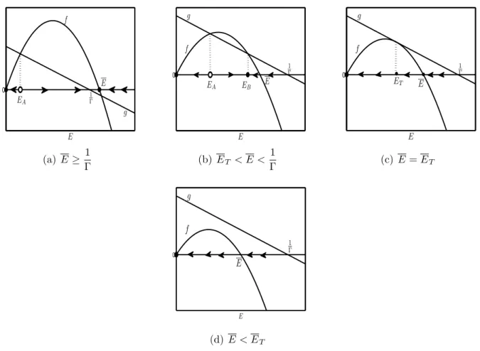
0 E EA Γ1 E f g (a) E≥ 1 Γ 0 E f g 1 Γ E EA EB (b) ET < E < 1 Γ 0 E f g E 1 Γ • ET • (c) E = ET 0 E f 1 Γ g E (d) E < ET
Figure 1: Dynamic regimes in the context η < η0, obtained by varying the carrying capacity E
of the natural resource. The other parameters are fixed at the values: β = 0.5, γ = 0.5, δ = 0.6, η = 0.073, r = 0.25, ET = 0.3575, 1/Γ = 0.5184.
The following proposition gives the complete taxonomy of the dynamic regimes which can be observed according to the dynamics (2). The proof of this proposition is straightforward and, for space constraints, will be omitted. Figures 1 and 2 illustrate all the dynamic regimes described in such proposition; full dots • and empty dots ◦ represent, respectively, attractive and repulsive stationary states.
Proposition 2 (1) In the context in which the condition η < η0 := 1/ (aΓ2) holds, the
fol-lowing dynamic regimes can be observed: (1.a) if E ≥ 1
Γ, then a unique interior stationary state EA ∈ (0, 1/Γ) exists, which is
repulsive and separates the basins of attraction of the locally attractive stationary states E = 0 and E = E (see figure 1(a));
(1.b) if 1
Γ > E > ET := 2
√
aη−aηΓ, then two interior stationary states EA and EB exist, with 0 < EA < EB < 1/Γ; the repulsive stationary state EA separates the basins of attraction of the locally attractive stationary states E = 0 and EB (see figure 1(b));6 (1.c) if E = ET, then two stationary state exist, E = 0 and E = ET :=
(
E + ηaΓ)/2 <
1/Γ, and their basins of attraction are respectively the intervals [0, ET) and [ET, +∞) (see figure 1(c));
6In the context η < η 0,
1
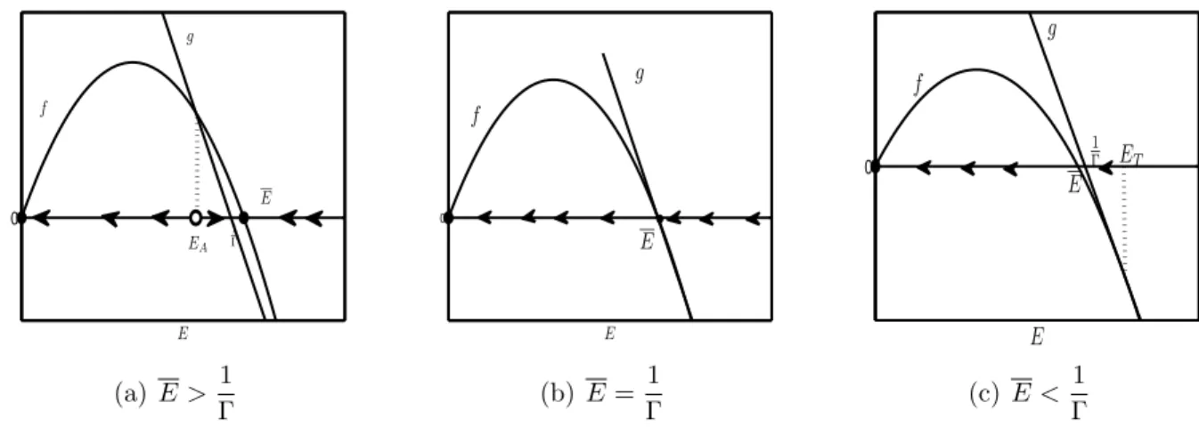
0 E 1 Γ E f g EA (a) E > 1 Γ 0 E f g E• (b) E = 1 Γ 0 E f 1 Γ g ET E (c) E < 1 Γ
Figure 2: Dynamic regimes in the context η ≥ η0, obtained by varying the carrying capacity E
of the natural resource. The other parameters are fixed at the values: β = 0.5, γ = 0.5, δ = 0.6, η = 0.4232, r = 0.25, ET = 0.5162, 1/Γ = 0.5184.
(1.d) if E < ET, then the stationary state E = 0 is globally attractive (see figure 1(d)). (2) In the context in which the condition η ≥ η0 holds, the following dynamic regimes can be
observed: (2.a) if E > 1
Γ, then the dynamic regime coincides with that described in point (1.a) of
this proposition (see figure 2(a)); (2.b) if E = 1
Γ, then two stationary states exist, E = 0 and E = E, and their basins of
attraction are respectively the intervals [0, E) and [E, +∞) (see figure 2(b)); (2.c) if E < 1
Γ, then the stationary state E = 0 is globally attractive (see figure 2(c)). The coordinates of the interior stationary states EA and EB (when existing) are given by:
EA= E + ηaΓ 2 − 1 2 √ (E + ηaΓ)2− 4ηa EB= E + ηaΓ 2 + 1 2 √ (E + ηaΓ)2− 4ηa (16)
Notice that in sub-case (1.a) of the above proposition, if E = 1
Γ, then EB = E holds. Further-more, in sub-case (1.c), EA= EB = ET holds; in such a case, the straight line f (E) is tangent
to the graph of g(E) at the point (ET, g(ET)) (see figure 1(c)).
Sub-cases (1.c) and (2.b) in Proposition 2 are “non-robust” in that they are associated with equality conditions on parameters’ values. The “robust” dynamic regimes described in Proposition 2 can be classified as follows: (1) the dynamic regimes associated to sub-cases (1.d) and (2.c), where the stationary state E = 0 is globally attractive; (2) the dynamic regimes associated to sub-cases (1.a)-(1.b) and (2.c), characterized by the coexistence of two locally attractive stationary states (bi-stable regime), the stationary state E = 0 and either the stationary state E = E or the stationary state EB. Bi-stable regimes occur only if the carrying
capacity E of the natural resource is high enough; notice that the coexistence between the local sector and the industrial sector can be observed only in the bi-stable regime corresponding
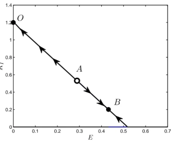
0 0.1 0.2 0.3 0.4 0.5 0.6 0.7 0 0.2 0.4 0.6 0.8 1 1.2 1.4 E KI B A O
Figure 3: The dynamics in the plane (E, KI) corresponding to the bi-stable regime illustrated in figure 1(b).
to sub-case (1.b) (see figure 1(b)), where the environmental impact (measured by η) of the industrial sector is low enough (η < η0) and the carrying capacity E of the environmental
resource belongs to the interval (ET, 1/Γ).
Remember that the equilibrium value of KI is determined by the equation KI =
(γδ
r
) 1 1−γ (1−
L) (see equation (7)), therefore KI is inversely proportional to L and, consequently, to E (see
equation(8)). Figure 3 shows the dynamics in the plane (E, KI) corresponding to the bi-stable
regime illustrated in figure 1(b). Notice that the stationary state with E = 0 is associated to the highest value of KI.
5
Revenues of L-agents
Taking into account that the equilibrium wage rate is w = δ(1− γ)(γδr)
γ
1−γ = a(1− γ), we can
prove the following proposition.
Proposition 3 ΠL(E) = Eβ holds for E ≥
1
Γ while ΠL(E) = [
Γ−β− a(1 − γ)]ΓE + a(1− γ)
holds for E < 1
Γ, where [
Γ−β− a(1 − γ)]> 0. That is, ΠL(E) is a strictly increasing function of E for every E ≥ 0. Consequently, in bi-stable regimes illustrated in figures 1(a)-(b) and 2(a), the attractive stationary states E = 0 is Pareto-dominated by the other attractive stationary states (either EB or E = E).
Proof. The revenues ΠL of the representative L-agent can be written as:
ΠL= EβL∗1−β+ (1− L∗)w = EβL∗1−β+ a(1− γ)(1 − L∗)
where L∗ = min{1, ΓE}. Thus ΠL= Eβ holds for E ≥ 1
Γ while: ΠL = Eβ(ΓE)1−β+ a(1− γ)(1 − ΓE) =
= Γ1−βE− ΓEa(1 − γ) + a(1 − γ) =
holds for E < 1
Γ. Notice that the condition:
Γ−β − a(1 − γ) = a(1− γ)
1− β − a(1 − γ) > 0
is always satisfied. This implies that ΠL is a strictly increasing function of E for every E ≥ 0.
According to the above proposition, in our model, an increase in KI is always associated to a
reduction in E and ΠL(see equation (7) and (8); this means that the environmental degradation
caused by the industrial sector produces a negative impact on labor remuneration which is always larger than the positive impact of the rise in labor productivity due to an increase in
KI. Consequently, in a bi-stable regime context, the locally attractive stationary state E = 0 is
always Pareto-dominated by the other locally attractive stationary states (E = EB or E = E)
and is associated to the highest value of KI; along the trajectory approaching it, the effort of
L-agents to defend themselves from environmental degradation drives the economy towards an undesirable complete specialization in the industrial sector. However, this does not imply that full specialization in the local sector always ensures the highest level of welfare for L-agents. In fact, the type of sectorial composition which is preferable depends on a set of conditions concerning the initial stock of natural capital, the pollution intensity of the industrial sector and the carrying capacity of the environmental resource in the host economy. In the following two sections we will clarify this observation.
6
Comparing the dynamics with and without external
investments
The effects generated by the external investments in our economy on L-agents welfare can be better understood by discussing more in detail the implications of the considered model in terms of environmental sustainability and by comparing the dynamics generated by the model (which will be called Dynamics with Externalities (DwE )) and the dynamics according to which L = 1 and KI = 0 hold for every E ≥ 0 (which will be called Natural Dynamics (ND)), namely the
dynamics that would be observed in absence of external investors.
Let us first specify the three main definitions of sustainability that we use (see Hanley et al. (1997), pp. 425-444). A trajectory followed by the economy is sustainable if:
(1) along it the welfare of local agents does not decrease;
(2) along it the stock E of the environmental resource does not decrease;
(3) it converges to a stationary state characterized by a strictly positive level of the natural resource (E > 0).
Taking into account the positive correlation between E and ΠL, in our model the condition (1)
is satisfied if and only if the condition (2) is satisfied. Furthermore, if a trajectory is sustainable according to the criteria (1)-(2), then it is sustainable according to the criterion (3).
In the ND -context, the environment is not affected by the polluting activity of the industrial sector, the time evolution of E is described by the logistic equation (12) and the revenues of L-agents are given by the function ΠN D
L (E) := Eβ. Under such dynamics, starting from every
initial value E(0) which satisfies the condition E ≥ E(0) > 0, the economy follows a trajectory along which ΠN DL and E increase and approaches the stationary state E = E, where the
revenues of L-agents are given by ΠN DL (E) = Eβ. Such a trajectory is therefore sustainable according to all the criteria (1)-(3).
In the DwE -context, we can observe that, according to Proposition 2, if the carrying capacity
E is sufficiently low (see the sub-cases (1.d) and (2.c) of Proposition 2), then the trajectory
followed by the economy is unsustainable according to all the criteria (1)-(3). In this case, the economy converges always to the stationary state E = 0, whatever the initial condition E(0) is, by following a trajectory along which the values of E and ΠL are always decreasing (while KI is increasing) (see figures 1(d) and 2(c)).
However, also in the DwE -context there exist trajectories along which E and ΠL are
in-creasing (and KI is decreasing) and all the criteria (1)-(3) are satisfied. These trajectories exist
only if either η ≥ η0 and E >
1
Γ (see figure 2(a), corresponding to sub-case (2.a) of Proposition 2) or η < η0 and E > ET (see figures 1(a) and 1(b), corresponding to sub-cases (1.a) and
(1.b) of Proposition 2), that is, if the carrying capacity E is high enough with respect to η. In fact, under these conditions, a bi-stable dynamic regime occurs and:
i) The economy follows a sustainable trajectory, according to all the criteria (1)-(3), if either
E(0) ∈ (EA, E], in the context of sub-cases (1.a) and (2.a) (see figures 1(a) and 2(a)), or E(0) ∈ (EA, EB], in the context of sub-case (1.b) (see figure 1(b)).
ii) The economy follows a trajectory along which E and ΠL are decreasing, which is
sustain-able according to the criterion (3) only, if E(0) > EB in the context of sub-case (1.b) (see
figure 1(b)).
iii) The economy follows a trajectory which is not sustainable according to all the criteria (1)-(3) if E(0) < EA.
Therefore, in a bi-stable regime context, sustainable trajectories according to all the criteria (1)-(3) can be observed only if the carrying capacity E and the initial endowment E(0) of the natural resource are high enough. It is worth stressing that the non transient coexistence between the two sectors of the economy is observed along a sustainable trajectory only if the stationary state EB exists (that is, only if the environmental impact of the industrial sector is
low enough, η < η0, and the carrying capacity satisfies the condition
1
Γ > E > ET) and if the initial endowment of the natural resource is such that E(0) > EA.
These results show that the openness to external investments does not exclude environ-mental sustainability and an improvement in the welfare of the local population even when the incoming capital is invested in polluting activities and it flows towards economies that are highly dependent on natural capital. The carrying capacity E, the initial stock of natural capital E(0) and the rate of environmental impact of the industrial sector η play a key role in determining the sustainability of the transition towards a diversified economic structure. Interestingly, the importance of the environmental factors is not limited by the fact that the economy is able to attract investments in activities that are not dependent on natural capital and local agents are able to shift from one sector to the other one. Furthermore, it is possible to demonstrate that a trajectory in the DwE -context may approach a stationary state, EB, which
Pareto-dominates the stationary state E = E in the ND -context, that is ΠL(EB) > ΠN DL (E).
Again, the conditions on which such a result is based depend crucially on the parameters E and
η. The following proposition highlights the conditions under which the value ΠN D
L (E) = E β
is higher than the value of ΠL(E) evaluated at the attractive stationary states of DwE, E = 0 and E = EB. The proof of such a proposition is straightforward and therefore it is omitted.
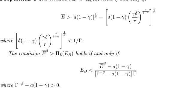
Proposition 4 The condition Eβ > ΠL(0) holds if and only if: E > [a(1− γ)]1β = [ δ(1− γ) ( γδ r ) γ 1−γ] 1 β (17) where [ δ(1− γ) ( γδ r ) γ 1−γ ]1 β < 1/Γ.
The condition Eβ > ΠL(EB) holds if and only if:
EB <
Eβ− a(1 − γ)
[Γ−β − a(1 − γ)] Γ (18)
where Γ−β− a(1 − γ) > 0.
In the bi-stable regime of sub-cases (1.a) and (2.a) in Proposition 2, starting from E(0) >
EA, the economy converges to the same stationary state of the natural dynamics, E = E;
consequently, ND and DwE drive the economy (in the long run) towards the same welfare level; however, starting from E(0) < EA, DwE approach the stationary state E = 0, where
ΠL(0) < E β
(being, in sub-cases (1.a) and (2.a), E ≥ 1/Γ). Thus, the long run effects on welfare generated by external investments depend crucially on the initial endowment E(0) of natural capital. However, in such a context (characterized by a high level of carrying capacity
E), the long run welfare in the DwE -context cannot be higher than the long run welfare in the ND -context.
In the bi-stable regime of sub-case (1.b) in Proposition 2, instead, the comparison across alternative stationary states in terms of local agents’ revenues is more ambiguous as suggested by Proposition 4. However, if the value of η is low enough, then Eβ < ΠL(EB) holds and
therefore the stationary state EB in the DwE -context Pareto-dominates the stationary state E = E in the ND -context; that is, a welfare improving coexistence between the two sectors can
be observed in a non transient way (that is, in a stationary state). In this case, the openness of the economy to external investors is beneficial for local agents’ revenues. External investment allows them to rely not only on activities that are limited by environmental constraints but also on sources of income which can grow over time through physical capital accumulation by I-agents. To check this result, remember that sub-case (1.b) is characterized by the conditions 1/Γ > E > ET := 2√aη− aηΓ and η < η0 := 1/ (aΓ2), where the values of a and Γ do not
depend on η while ET → 0 for η → 0. Consequently, given E < 1/Γ, such conditions are
always satisfied if η is low enough. Furthermore, being E < 1/Γ, in E = E it holds L < 1 in the DwE -context and consequently Eβ < ΠL(E) (because, in the DwE -context, the revenues
are maximized with respect to L, given the value of E). This implies that, by the continuity of the function ΠL(E), E
β
< ΠL(EB) holds if EB is near enough to E. In fact, this is just the
case when η is low enough in that EB → E for η → 0 (see equation (16)).
The value of the parameter η plays a key role in our model. If η increases, then EB
decreases, being ∂EB/∂η < 0 (see (16)), and the condition (18) will be more easily satisfied.
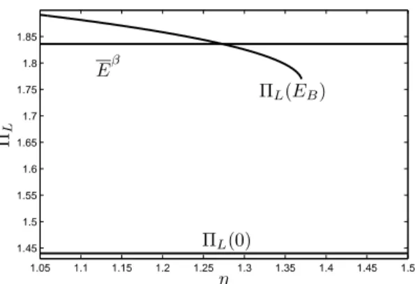
Figure 4 compares the value of ΠN DL (E) = Eβ with the values of ΠL(E) in the locally attractive
stationary states E = 0 and EB (ΠL(0) and ΠL(EB), respectively). In such numerical exercise,
ΠL(0) corresponds to the minimum level of local agents’ welfare; moreover, ΠL(EB) > E β
holds for low enough values of η while the opposite inequality holds for higher values of η. When
1.05 1.1 1.15 1.2 1.25 1.3 1.35 1.4 1.45 1.5 1.45 1.5 1.55 1.6 1.65 1.7 1.75 1.8 1.85 η ΠL ΠL(0) ΠL(EB) Eβ
Figure 4: The value of revenues of local agents in the stationary state E = E (Eβ) of the
Natural Dynamics, compared with the revenues in the locally attractive stationary states E = 0
and E = EB (ΠL(0) and ΠL(EB), respectively) of the Dynamics with Externalities, obtained by varying the value of the rate of pollution η. The other parameters are fixed at the values: β = 0.485, γ = 0.5, δ = 1.2, r = 0.25, E = 3.5.
both the stationary states E = 0 and EB in the DwE -context are Pareto-dominated by the
stationary state E = E in the ND -context, then external investments always generate a long run reduction in local agents’ welfare. However, when EB Pareto-dominates E = E which,
in turn, Pareto-dominates E = 0, the long run effects of external investments depend on the initial endowment E(0) of the natural resource: DwE will do better than ND if E(0) > EA,
vice versa if E(0) < EA.
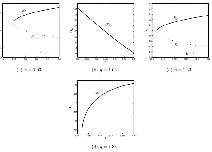
Some other numerical exercises, varying the parameters η and r, may be useful to illustrate the effects of a variation in these parameters on the values of EA, EB and ΠL(EB). Figures
5(a)-(b) report the impact of an increase in η while figures 6(a)-(d) illustrate the impact of a change in r for two different levels of η. Observe that, when η increases, the values of EB
and ΠL(EB) become lower, and this implies an increase in KI.7 When η increases, the local
community faces a reduction in E and therefore in the productivity of self-employed labor and local agents are pushed towards wage employment. In this context, the expansion of external capital inflows does not help local agents in that their welfare (evaluated at the stationary state
EB) declines. It is worth noting that these outcomes emerge even if the labor market is perfectly
competitive and is not segmented, that is, in a context where a rise in labor demand by the industrial sector produces a pattern of labor reallocation that could raise labor remuneration in both sectors. The introduction of environmental externalities, instead, mitigates the effects of this channel of transmission resulting in an expansion of output share of the industrial sector with constant wages and a decrease in local agents’ welfare. Indeed, as reported in Proposition 1, the equilibrium wage rate is constant and is not affected by variations in the parameter
η. A reduction in r, instead, has a positive impact on the wage rate. In fact, a decline in r
represents a decrease in external agents’ opportunity cost of capital investment in the economy. The consequent inflows of external capital produce an increase in labor productivity in the industrial sector and, as a result, also in labor remuneration. However, the net impact on ΠL
also depends on the value of η. For a sufficiently low η (figures 6(a)-(b)), a decrease in r leads to a growth of ΠL(evaluated at EB) though it causes also a decline in EB. As shown in figures
6(c)-(d), for a higher value of η, however, the opposite is true and a reduction in r generates a reduction in local agents’ welfare and in EB.
7Notice also that the size of the basin of attraction of E
0 0.5 1 1.5 0 0.5 1 1.5 2 2.5 3 3.5 4 4.5 5 η E E = 0 EB EA (a) 0 0.5 1 1.5 1.8 1.85 1.9 1.95 2 η ΠL ΠL(EB) (b)
Figure 5: The values of EA, EB and ΠL(EB) obtained by varying the value of the rate of pollution η. The parameter values are the same used in the numerical exercise illustrated in figure 4.
7
Optimal economic dynamics
The inability of local agents to coordinate their choices might represent the main obstacle to sustainable development in the economy under consideration here. This section discusses the potential contribution of a social planner’s intervention which ensures that environmental externalities are taken into account in the choice of labor allocation between the local and the industrial sector, made up of resource-dependent and resource-impacting activities. In this section we analyze the dynamics of the economy under the assumption that the labor input L of the representative local agent is chosen by a social planner which has the aim of maximizing the value of the objective function:
+∞
∫
0
(ΠL)· e−σtdt (19)
where the parameter σ > 0 measures the time preference of the representative L-agent, which can also be interpreted as a measure of altruism with respect to future generations. To express the value of the revenues ΠL= EβL1−β+ (1− L)w in terms of E and L only, we have to take
into account that the representative external investor chooses 1− L and KI in order to satisfy the first order conditions (4) and (5), given respectively by:
δ(1− γ)KIγ(1− L)−γ = w
δγKIγ−1(1− L)1−γ = r Notice that, by the latter condition,
KI = (δγ
r )
1
1−γ(1− L) (20)
holds; by substituting (20) in the former condition, we obtain the value of the equilibrium wage rate w which, substituted in ΠL, allows us to write:
ΠL(E, L) = EβL1−β + δ(1− γ) ( δγ r ) γ 1−γ (1− L)
0.2 0.21 0.22 0.23 0.24 0.25 0 0.5 1 1.5 2 2.5 3 r E EA EB E = 0 (a) η = 1.03 0.22 0.225 0.23 0.235 0.24 0.245 0.25 1.89 1.9 1.91 1.92 1.93 1.94 1.95 1.96 1.97 r ΠL ΠL(EB) (b) η = 1.03 0.245 0.246 0.247 0.248 0.249 0.25 1.5 1.6 1.7 1.8 1.9 2 2.1 2.2 2.3 2.4 2.5 r E E = 0 EA EB (c) η = 1.33 0.245 0.246 0.247 0.248 0.249 0.25 1.785 1.79 1.795 1.8 1.805 1.81 r ΠL ΠL(EB) (d) η = 1.33
Figure 6: The values of EA, EB and ΠL(EB) obtained by varying the cost r of KI, with η = 1.03 (figures 6(a)-6(b)) and η = 1.33 (figures 6(c)-6(d)). The other parameter values are the same used in the numerical exercise illustrated in figure 4.
The social planner, therefore, has to choose the function L(t), t ∈ [0, +∞), that solves the following optimization problem:
M AX L +∞ ∫ 0 [ EβL1−β + a(1− γ)(1 − L)]e−σtdt (21) subject to the constraints:
˙ E = E(E− E) − ηa(1 − L) E ≥ 0, 0 ≤ L ≤ 1, where a := δ ( γδ r ) γ 1−γ
. Notice that the maximization problem (21) satisfies Mangasarian’s sufficient conditions; consequently, we have that if a growth path satisfies the conditions of the Maximum Principle and the usual transversality condition lim
t→+∞E(t)· λ(t) · e−σt = 0, where λ is the co-state variable associated to E, then it is a solution of problem (21).
The current value Hamiltonian function associated to the problem (21) is:
H(E, λ, L) = ΠL(E, L) + λ
[
E(E− E) − ηa(1 − L)]
0 0.05 0.1 0.15 0.2 0.25 0 0.1 0.2 0.3 0.4 0.5 0.6 0.7 0.8 0.9 1
E
L
E
∞ BE
∞ AE
∞ C˙
L = 0
˙
E = 0
Figure 7: Bi-stable regime in the Dynamics with Social Planner-context: if the initial value
E(0) of the state variable E is such that 0 < E(0) < EA∞ (respectively, E(0) > EA∞), then the initial value L(0) of the jumping variable L will be fixed so that the trajectory starting from (E(0), L(0)) belongs to the stable branch of EC∞ (respectively, of EB∞). Parameter values: β = 0.485, γ = 0.5, δ = 0.5, η = 0.005, σ = 0.1, r = 0.25, E = 0.1. ˙ E = ∂H ∂λ = E(E− E) − ηa(1 − L) (22) ˙λ = σλ − ∂H ∂E = (σ− E + 2E)λ − β ( L E )1−β (23) where, in each instant of time, the value of L∈ [0, 1] is given by the solution of the problem:
M AX
L H(E, λ, L) (24)
Notice that if L = 1 solves problem (24), then the system (22)-(23) becomes:
˙ E = E(E− E) ˙λ = (σ − E + 2E)λ − β ( 1 E )1−β
Such system admits a unique stationary state with E = E and λ = β (σ + E)E1−β
. When problem (24) admits an interior solution (that is, L ∈ (0, 1)), then L must satisfy the first order condition: ∂H ∂L = (1− β) ( E L )β − a(1 − γ) + ληa = 0 (25)
0
a)
b)
E
•
E
E
∞ CE
∞ AE
∞ BE
BE
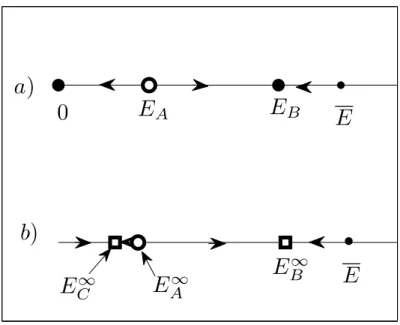
AFigure 8: Bi-stable regime in the Dynamics with Externalities-context (figure 8(a)), obtained
with the same parameter values used in the simulation of figure 7, and the projection on the E−axis of the trajectories belonging to the stable branches of EC∞ and EB∞ in figure 7 (figure 8(b)).
By solving (25) with respect to λ:
λ = 1 ηa [ a(1− γ) − (1 − β) ( E L )β] (26)
and by substituting λ in (23), we can write: ˙λ = 1 ηa(σ− E + 2E) [ a(1− γ) − (1 − β) ( E L )β] − β ( L E )1−β (27)
Finally, deriving with respect to time both sides of the equation (25), we obtain: ˙ L L = ˙ E E + σ− E + 2E β(1− β) [ (1− γ)a ( L E )β − 1 + β ] − ηa 1− η ( L E ) (28)
which represents the time evolution of L when L ∈ (0, 1) and, consequently, the trajectories that the economy can follow are determined by the dynamic system (22), (28). These dynamics will be called Dynamics with Social Planner (DSP ).
It is easy to check that, according to (25), the optimal level of L is always higher (ceteris paribus) than the value chosen by the representative L-agent in the Dynamics with Externalities (see (6) and (7)). This is the case because the social planner takes into account of the “price”
λ of the natural resource when she chooses L. In this way, the social planner is able to contain
an excessive use of wage labor which increases L-agents’ revenues in the short run, but leads to a reduction in ΠL in the long run due to environmental degradation. Local agents can
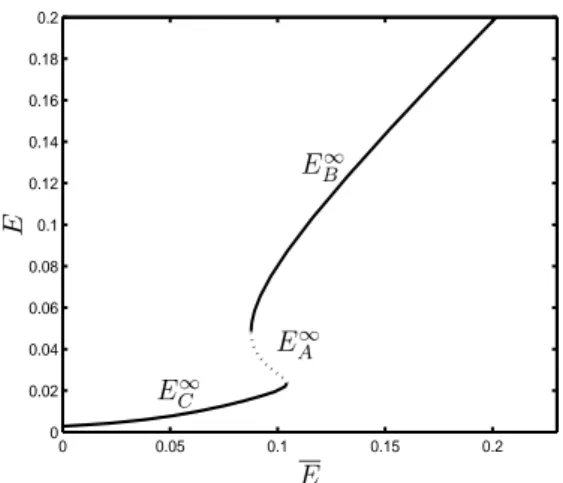
0 0.05 0.1 0.15 0.2 0 0.02 0.04 0.06 0.08 0.1 0.12 0.14 0.16 0.18 0.2 E E E∞ B E∞ C E∞ A
Figure 9: The values of EA∞, EB∞ and EC∞, obtained by varying the value of the carrying capacity E; the other parameter values are the same used in the simulation in figure 7. The continuous lines indicate the saddle-point stable stationary states while the dotted line indicates the repulsive stationary state EA∞ .
choose to allocate more time to the industrial sector in order to defend themselves against low productivity levels in the local sector, due to low values of E; this defensive strategy, however, generates a further reduction in E which, in turn, leads to an additional increase in the labor input in the industrial sector and so on. This vicious process is self-enforcing and may drive the economy towards the complete depletion of the natural resource, as we have shown in the preceding sections. Unlike local agents, the social planner is able to internalize the negative effects generated by such a self-enforcing process and to let the economy to follow a trajectory along which external investments allow for the maximization of the value of the discounted flow of revenues (19).
Due to space constraints, we shall not provide a complete analysis of the system (22), (28) but we limit our study to some numerical simulations which have the objective of illustrating some differences between the DwE and DSP -contexts. In the simulation showed in figure 7, three stationary states EA∞, EB∞ and EC∞ exist. The states EB∞ and EC∞ are saddle points, and their stable branches are indicated in bold, while EA∞ is repulsive. If the initial value E(0) of the state variable E is such that 0 < E(0) < EA∞ (respectively, E(0) > EA∞), then the initial value L(0) of the jumping variable L will be fixed so that the trajectory starting from (E(0), L(0)) belongs to the stable branch of EC∞ (respectively, of EB∞). Figure 8(a) illustrates the trajectories of the DwE, obtained with the same parameter values used in the simulation of figure 7, and figure 8(b) shows the projection on the E−axis of the trajectories belonging to the stable branches of EC∞ and EB∞ in figure 7. Notice that the attractive stationary states E = 0 and EB, in figure 8(a), have been “replaced” by, respectively, the saddle-point stable stationary
states EC∞and EB∞in figure 8(b), with 0 < EC∞and EB < EB∞. Thus, in this numerical example,
the complete environmental depletion is avoided in the DSP -context. The repulsive points EA
and EA∞ separate (along the E−axis) the basins of attraction of E = 0 and EB and of EC∞ and EB∞, respectively. Figure 9 illustrates how the values of EA∞, EB∞ and EC∞ change with the varying value of the carrying capacity E. The continuous lines indicate the saddle-point stable stationary states while the dotted line indicates the repulsive stationary state EA∞. Notice that if the carrying capacity E is low enough or high enough, then only one stationary state exists, while for intermediate values of E the bi-stable regime illustrated in figure 7 is observed.
0 20 40 60 80 100 120 140 160 180 0.315 0.32 0.325 0.33 0.335 0.34 0.345 0.35 t ΠL ( t) ΠDwE (t) ΠN D (t) ΠDS P (t) (a) 0 20 40 60 80 100 120 140 160 180 0.075 0.08 0.085 0.09 0.095 0.1 0.105 t E (t ) EDwE(t) EN D (t) EDS P(t) (b)
Figure 10: The time evolution of L-agents’ revenues ΠL and of the stock E along trajectories starting from the same initial value E(0). The graphs of the functions EN D(t), EDwE(t), EDSP(t) represent, respectively, the time evolution of E in the ND, DwE, DSP-contexts, while
those of the functions ΠN D
L (t), ΠDwEL (t), ΠDSPL (t) illustrate the corresponding time evolution of the revenues along such trajectories. The initial value E(0) is such that EN D(t), EDwE(t), EDSP(t) approach, respectively, the stationary state values E, EB, EB∞, with E > EB∞ > EB. The parameter values are the same used in the simulation in figure 7 .
capital may play a key role in determining the optimal trajectory followed by the economy. The role played by E(0) in the alternative ND, DwE and DSP -contexts is clearly shown in figures 10 and 11, which illustrate the time evolution of L-agents’ revenues and of E along trajectories starting from the same initial value E(0). In these figures, the graphs of the functions EN D(t), EDwE(t), EDSP(t) indicate, respectively, the time evolution of E in the ND, DwE, DSP -contexts, while those of the functions ΠN D
L (t), ΠDwEL (t), ΠDSPL (t) illustrate the
corresponding time evolution of the revenues along such trajectories. In figure 10, the initial value E(0) is such that EN D(t), EDwE(t), EDSP(t) approach, respectively, the stationary state
values E, EB, EB∞, with E > EB∞> EB. Notice that the value of ΠDSPL (t) becomes definitively
higher than the value of ΠDwEL (t) and the value of ΠDwEL (t) is always higher that the value of ΠN D
L (t). Consequently, in this example, Natural Dynamics do not give rise to the highest long
run welfare level. This result is reversed if the economy starts from a lower initial value E(0), as it is shown in figure 11 where EN D(t), EDwE(t), EDSP(t) approach, respectively, the stationary state values E, 0, EC∞, with E > EC∞ > 0, and the value of ΠN D
L (t) becomes definitively higher
than the values of ΠDwE
L (t) and ΠDSPL (t). This result is not surprising if we take into account
that the objective function (19) discounts future values of ΠL at the discount rate σ > 0.
Our simulations confirm that the initial endowment E(0) affects the ranking of the long run welfare outcomes in the alternative contexts (ND, DwE and DSP ) under consideration here. If the initial value E(0) is high enough (that is, E(0) > EA and E(0) > EA∞ in the DwE
and DSP -contexts, respectively), both DwE and DSP meet the third criterion of sustainability (that is, a strictly positive stationary value of E is reached), converge to a stationary state in which both sectors coexist and are associated, in every instant of time, to higher levels of ΠL than in the ND - context (figure 10). Under these conditions, along the optimal trajectory,
a gradual reduction in natural capital is observed which implies an increase in investment in physical capital and a progressive expansion of the industrial sector. In other words, in this numerical example, the absence of external investment does not lead to the highest level of ΠL
either at each instant of time or in terms of the discounted value of future revenues.
-0 10 20 30 40 50 0.1 0.15 0.2 0.25 0.3 t ΠL ( t) ΠN D L (t) ΠDSP L (t) ΠDwE L (t) (a) 0 10 20 30 40 50 −0.02 0 0.02 0.04 0.06 0.08 0.1 t E (t ) EDS P (t) EDwE(t) EN D(t) (b)
Figure 11: The time evolution of L-agents’ revenues ΠL and of the stock E along trajectories starting from the same initial value E(0). The initial value E(0) is such that EN D(t), EDwE(t), EDSP(t) approach, respectively, the stationary state values E, 0, EC∞, with E > EC∞ > 0. The parameter values are the same used in the simulation in figure 7 .
contexts (figure 11). Also in this case, the maximization of the objective function (19) implies a convergence to a diversified economy without specialization. Moreover, the optimal solution corrects the factors of unsustainability which affect the dynamics without social planning and, in fact, it meets all criteria of sustainability (while dynamics with externalities is unsustainable according to all adopted definitions). Nevertheless, in the context of figure 11, both DwE and
DSP generate long run welfare values which are lower than that generated by ND. In such a
case, the trajectory followed by ND is preferable to the trajectories followed by DwE and DSP if the criterion of optimality is the maximization of ΠLevaluated at the stationary state reached
by the trajectory instead of the maximization of the objective function (19).
8
Conclusions
We have analyzed an economy where local agents rely on free access to natural resources and where they can defend themselves from environmental degradation by providing labor to the industrial sector which is not dependent on natural capital. Moreover, the source of capital for the industrial sector is “unlimited” in that external investors can raise funds in financial markets and invest in physical capital in this economy as long as the return on capital generated is higher than in other economies. The labor market is perfectly competitive and inter-sector labor movement is free and without cost. In such a context, we could expect that an increase in capital investments in the industrial sector leads to a raise in welfare of local agents. Our analysis, instead, shows that the introduction of the environmental impact of the industrial sector mitigates, and in some cases reverses, this effect. In particular, in the economy under consideration here, opposite scenarios are admissible: (a) the economy may converge to the stationary state E = 0, following an undesirable self-enforcing growth process of the industrial sector, associated with environmental unsustainability and impoverishment of the local population; (b) it may undertake a sustainable transition towards a diversified economic structure and converge to the stationary state E = EB > 0, where both sectors
coexist; (c) it may drive out capital inflows and converge to the unique attractive stationary state (E = E) of the “natural dynamics”, namely the dynamics that would be observed in absence of external investors. The type of path that is selected and which is preferable in
terms of local agents’ welfare and environmental sustainability depends on a set of conditions concerning the initial stock E(0) of natural capital, the pollution rate η of the industrial sector and the carrying capacity E of the environmental resource in the host economy. The paper identifies and discusses these conditions and shows how they affect the number and the stability of the stationary states as well as their welfare properties. In particular, our analysis shows that if the economy starts from a low enough value of E(0), whatever are the values of η and E, then the scenario (a) will be observed. If the values of E(0) and E are high enough, whatever is the value of η, then the scenario (c) will occur. Finally, the scenario (b) will take place only if η is low enough, E(0) is high enough and E is neither too low nor too high; this is the unique scenario in which both sectors coexist in a non transient way.
In our economy, the environmental degradation (that is, the reduction in E) caused by the industrial sector always produces a reduction in the welfare of local populations, which is positively correlated with E. However, we find that this result does not imply that full specialization in the local sector always ensures the highest level of welfare for local agents. Under strict conditions, spelt out in the paper, scenario (b) is preferable to scenario (c), that is the arrival of external capital inflows and the convergence to the stationary state with the coexistence of both sectors leads to a higher welfare level among local agents than the absence of external investments, even in a context in which environmental negative externalities are not internalized by a social planner. The coordination of labor allocation choices by a social planner can avoid the complete exhaustion of natural capital (scenario (a)) and, in all other scenarios, can ensure higher levels of welfare than the dynamics without internalization of environmental externalities.
In poor economies, inflows of external investments are seen by policy makers as the main solution to tackle scarcity of domestic capitals and to escape a poverty trap of low investments, low growth and poverty perpetuation. The arrival of external investors is considered to be beneficial for economic expansion and diversification of the local economy.
Our results suggest that environmental preservation and protection should be considered as a complementary rather than a supplementary measure to the openness to inflows of external investment in impacting sectors even in an economy where barriers to labor movement do not represent an obstacle towards full specialization in the incoming activities which are not dependent on environmental resources. Environmental defense, in the form of support to the initial endowment of natural capital and to the environmental carrying capacity, and limitation to pollution impact of external investment are prerequisites for a welfare improving coexistence between the two sectors in the economy we have analyzed.
References
Alfaro, L., A. Chanda, S. Kalemli-Ozcan, and S. Sayek (2004). Fdi and economic growth: the role of local financial markets. Journal of International Economics 64 (1), 89–112.
Alguacil, M., A. Cuadros, and V. Orts (2011). Inward fdi and growth: The role of macroeco-nomic and institutional environment. Journal of Policy Modeling 33 (3), 481 – 496.
Amiti, M. and K. Wakelin (2003). Investment liberalization and international trade. Journal
of International Economics 61 (1), 101–126.
Antoci, A. (2009). Environmental degradation as engine of undesirable economic growth via self-protection consumption choices. Ecological Economics 68 (5), 1385–1397.
Antoci, A. and S. Bartolini (2004). Negative externalities, defensive expenditures and labour supply in an evolutionary context. Environment and Development Economics 9 (05), 591–612. Antoci, A., P. Russu, and E. Ticci (2009). Distributive impact of structural change: Does environmental degradation matter? Structural Change and Economic Dynamics 20 (4), 266– 278.
Antoci, A., P. Russu, and E. Ticci (2012). Environmental externalities and immiserizing struc-tural changes in an economy with heterogeneous agents. Ecological Economics 81 (C), 80–91. Aykut, D. and S. Sayek (2007). The role of the sectoral composition of foreign direct investment on growth. In L. Piscitello and G. Santangelo (Eds.), Do multinationals feed local development
and growth?, pp. 35–62. Amsterdam:Elsevier.
Balasubramanyam, V. N., M. Salisu, and D. Sapsford (1996). Foreign direct investment and growth in ep and is countries. Economic Journal 106 (434), 92–105.
Barbier, E. B. (2010). Poverty, development, and environment. Environment and Development
Economics 15 (06), 635–660.
Barrios, S., H. Goerg, and E. Strobl (2003). Explaining firms’ export behaviour: R & D, spillovers and the destination market. Oxford Bulletin of Economics and Statistics 65 (4), 475–496.
Blomstrom, M., R. Lipsey, and M. Zejan (1994). What explains developing country growth? NBER Working Papers 4132, National Bureau of Economic Research, Inc.
Borensztein, E., J. De Gregorio, and J.-W. Lee (1998). How does foreign direct investment affect economic growth? Journal of International Economics 45 (1), 115–135.
Brems, H. (1970). A growth model of international direct investment. American Economic
Review 60 (3), 320–31.
Chakraborty, C. and P. Nunnenkamp (2008). Economic reforms, fdi, and economic growth in india: A sector level analysis. World Development 36 (7), 1192–1212.
Chang, N. (2012). The empirical relationship between openness and environmental pollution in china. Journal of Environmental Planning and Management 55 (6), 783–796.
Chomitz, K. (2008). At loggerheads? agricultural expansion, poverty reduction, and environ-ment in tropical forests. World Bank Policy Research Report, Washington D.C.
De Janvry, A. and R. Garcia (1988). Rural poverty and environmental degradation in latin america: causes, effects and alternative solutions. S88/L.3/Rev.2, Rome: IFAD.
de Mello Jr., L. R. (1997). Foreign direct investment in developing countries: A selective survey. Studies in economics, Department of Economics, University of Kent.
Easterly, W. (2006). Reliving the 1950s: the big push, poverty traps, and takeoffs in economic development. Journal of Economic Growth 11 (4), 289–318.
Economy, E. C. (2004). The river runs black: the environmental challenge to China’s future. Ithaca & London: Cornell University Press.