Assessment of damage to people and buildings as consequence of hydrogen pipeline accidents

(1)

i

University of Rome “Sapienza”

Department of Chemical Engineering, Materials and Environment

ASSESSMENT OF DAMAGE TO PEOPLE

AND BUILDINGS AS CONSEQUENCE OF

HYDROGEN PIPELINE ACCIDENTS

PhD in Chemical Engineering

XXXII cycle

Tutor Candidate

Prof.ssa Paola Russo Alessandra De Marco

(2)

ii

Publications list

International Journals

Russo P., De Marco A., Mazzaro M., Capobianco L., 2018, Quantitative risk assessment on

a hydrogen refuelling station, Chemical Engineering Transactions, 67, pp. 739-744.

Russo P., De Marco A., Parisi F., 2019, Failure of concrete and tuff stone masonry buildings

as consequence of hydrogen pipeline explosions, International Journal of Hydrogen Energy,

44, pp. 21067- 21079.

Conference proceedings

Russo P., De Marco A., Parisi F., 2018, Failure probability of reinforced concrete buildings

as consequence of hydrogen pipeline explosions, In: HYPOTHESIS XIII, Book of Abstracts,

Lecture A9/3, Singapore, 24-28 July 2018.

Russo P., De Marco A., Parisi F., 2019, Impact assessment on people and buildings for

hydrogen pipeline explosions, Proceedings of 8th International Conference on Hydrogen

(3)

iii

Abstract

Hydrogen is increasingly considered a valid alternative to traditional fuels, which are gradually being more and more depleted. It is defined as “the energy carrier of the future” and so, as such, it must be produced. Several hydrogen production technologies are widespread and they involve both traditional and innovative sources.After its production, the hydrogen must be made available for use and, so, it must be transported from the production site to the utilization site.

One of the most common ways to transport considerable quantities of gaseous hydrogen is through pipelines.

Since hydrogen is considered a “no safe” fuel due to its physical properties, the consequences of an accidental release must be investigated, to preserve the safety of people and facilities located in the surrounding area of a possible accidental event involving pipelines.

Hydrogen disperses into the air very easily, being lighter than air, but if it is released in a confined space can result in an explosion.

The hazards of the hydrogen-air mixture are related to the wide flammability range and the low minimum ignition energy. Furthermore, hydrogen burns with an invisible flame and so it is very difficult to suddenly identify the presence of danger.

Based on these considerations, it results that a failure of pipeline conveying gaseous hydrogen can pose severe risks.

The aim of this study is to evaluate damage to people and buildings involved in high-pressure hydrogen pipeline explosions and (jet) fires and, to this scope, a probabilistic risk assessment procedure is proposed.

The annual probability of damage to people and to buildings exposed to an extreme event is calculated as the product of the conditional probability of damage given by a fire or an explosion and the probability of occurrence of the fire/explosion as consequence of pipeline failure.

The consequences of hydrogen pipeline accidents are estimated through different tools: the SLAB integral model is used to define the gas dispersion, the TNO Multi-Energy Method to evaluate the overpressure and impulse generated from the explosions and Pressure-Impulse diagrams to evaluate damage to buildings.

(4)

iv The flame length is calculated through the SLAB model by considering the length at which the hydrogen concentrations of 4% (lower limit flammability) is reached.

The point source model is employed to estimate the radiative heat flux generated by jet fire with the radiant fraction calculated through the empirical correlation proposed by Molina et al. (2007).

Finally, the Probit equations are used to calculate damage to people, both in the case of an explosion and a jet fire. The characteristic quantities of the two accidental events investigated, overpressure and impulse in the case of the explosions and radiative heat flux in the case of jet fires, are considered as causative variables.

Reinforced concrete buildings and tuff stone masonry buildings are taken into consideration to estimate the effect of overpressure and impulse caused by an explosion.

Direct and indirect damage on the people are investigated to define the effects of consequence of explosions and jet fires.

The probabilistic procedure proposed can represent a useful tool in the design of a new hydrogen distribution network and in risks assessment for existing ones.

(5)

v

List of Figures

CHAPTER 1

Figure 1.1: Hydrogen jet fire and gasoline fire 2

Figure 1.2: The phase diagram of hydrogen 3

Figure 1.3: Momentum-controlled jet, transitional jet and buoyancy-controlled for a

horizontal jet. 5

CHAPTER 2

Figure 2.1: Hydrogen Production plant distribution in the World 9

Figure 2.2: Capacity (Nm3_{/h) of hydrogen production plants} ₁₀

Figure 2.3: Main causes of accidents involving hydrogen (data from Gerboni and Salvator,

2019) 12

Figure 2.4: Example of an event tree constructed for a failure of a pipeline carrying hydrogen

(data from Gerboni and Salvator, 2019) 14

CHAPTER 3

Figure 3.1: A free expansion gas leak 17

Figure 3. 2: Characteristic plume following a continuous release and puff following an

instan-taneous gas release 19

Figure 3.3: Dispersion cloud in the plume dispersion model by SLAB 22

Figure 3.4: Experimental setup related to the trials of Shirvill et al. (2006) 23

Figure 3.5: Comparison of hydrogen concentration (expressed in terms of volume fractions)

vs distance between SLAB predictions and experimental data by Shirvill et al. (2006) in the

conditions of RUN 3 25

Figure 3. 6: Comparison of hydrogen concentration (expressed in terms of volume fractions)

(9)

ix

Figure 3. 8: Comparison of hydrogen concentration (expressed in terms of volume fractions)

Figure 3.9: Experimental setup considered by Han et al. (2014) 27

vs distance between SLAB predictions and experimental data by Han et al. (2014) (P=100

bar, df= 1 mm) 28

bar, df= 1 mm) 29

vs distance between SLAB predictions and experimental data related to Okabayashy et al.

(2005) 31

Figure 3.1 4: Predicted values of hydrogen concentration vs experimental values of hydrogen

concentration, expressed in terms of volume fraction 31

Figure 3. 15: Blast wave pressure at fixed location 32

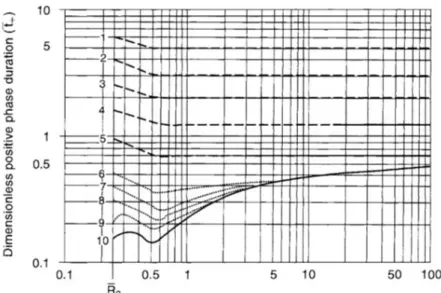
Figure 3. 16: Sachs-scaled positive -phase duration for the TNO model by Crowl and Louvar

(2011) 34

Figure 3. 17: Sachs-scaled “side-on” overpressure for the TNO model by Crowl and Louvar

(2011) 34

Figure 3. 18: Interaction of a blast wave with a rigid structure (Crowl, 2013) 40

Figure 3. 19: Pressure-impulse diagrams of RC column at multiple damage levels 43

(10)

x

Figure 3. 21: Pressure-impulse diagrams for different pre-compression levels 45

Figure 3.22: Parameters that characterize the flame shape: flame length (Lf) and flame width

(Wf) (Imamaura et al, 2008) 49

Figure 3.23: Validation of flame length evaluated with literature correlation and with SLAB

against experimental data 51

Figure 3.24: Single point source model (Hankinson and Lowesmith, 2012) 52

Figure 3.25: Variation of radiative fraction (χrad) with the factor τG αP Tf4 for different

hydrocarbon flames, proposed by Molina et al. (2007) 53

Figure 3.26: Weighted multi point source model by Hankinson and Lowesmith (2012) 54 Figure 3.27: Line source model by Zhou and Jiang (2016) 56

Figure 3.28: Experimental apparatus (Mogi et al., 2009) 59

Figure 3.29: Validation of procedure for the heat flux prediction against experimental data

59

CHAPTER 4

Figure 4.1: Peak of overpressure (a) and impulse (b) versus hole diameter at different value

of operating pressure (d=0.508 m, L=1000 m, R=500 m, atmospheric stability class D, v= 5

m/s, explosivity class 9) 67

Figure 4.2: Peak of overpressure (a) and impulse (b) versus hole diameter at different value

of operating pressure (d=0.508 m, L=1000 m, R=500 m, atmospheric stability class D, v= 5

m/s, explosivity class 9) 68

Figure 4.3: Blast probability for the blast strength 6 and atmospheric stability classes D5(a)

and F2 (b) 69

Figure 4.4: Blast probability for the blast strength 9 and atmospheric stability classes D5(a)

and F2 (b) 70

Figure 4.5: Comparison between blast demand and capacity of RC columns for explosivity

class 6 (a) and 9 (b), for atmospheric conditions D5 and F2 72

Figure 4.6: Comparison between blast demand and capacity of TSM walls for explosivity

class 6 (a) and 9 (b), for atmospheric conditions D5 and F2 73

(11)

xi

Figure 4.8: Structural components over the building façade 76

Figure 4.9: Assessment of blast impact on structural components Pier 1 (a) and Pier 2 (b)

77

Figure 4.10: Natural gas pipelines: Peak of overpressure (a) and impulse (b) versus hole

diameter at different value of operating pressure (d=1.257 m, L=1000 m, R=500 m,

atmospheric stability class C, v= 10 m/s, explosivity class 6) 78

Figure 4.11:Natural gas pipelines: Peak of overpressure (a) and impulse (b) versus pipeline length from the centre of compression at different value of pipeline diameters (Po=5000 kPa,

R=500 m, full bore rupture, atmospheric stability class C, v= 10 m/s, explosivity class 6) 79

Figure 4.12: Probability of death due to lung haemorrhage for explosive class 9 and

atmos-pheric stability class F2 82

Figure 4.13: Probability of death due to head impact for explosive class 9 and atmospheric

stability class F2 82

Figure 4.14: Probability of death due to whole body impact for explosive class 9 and

Figure 4.15: Probability of injury due to eardrum rupture for explosive class 9 and

Figure 4.16: Radiative heat flux versus hole diameter (d=0.508 m, r= 200 m,L=1000 m,

atmospheric stability class F, v= 2 m/s) 85

Figure 4.17: Radiative heat flux versus hole distance to the center of the jet fires (d=0.508 m, dhole

= d (full rupture) ,L=1000 m, atmospheric stability class F, v= 2 m/s) 85

Figure 4.18: Probability of fatality due to radiative heat flux (W/m2 ) at different distances

at t=60 s 87

Figure 4.19: Probability of overall injuries due to radiative heat flux (W/m2 ) at different

distances at t=60 s 88

Figure 4.20: Probability of injury due to first-degree burns at different distances at t=60 s

88

Figure 4.21: Probability of injury due to second-degree burns at different distances at t=60 s

(12)

xii

Figure 4.22: Probability of fatality due to radiative heat flux (W/m2 _{) at different distances}

at t=300 s 90

Figure 4.23: Probability of overall injuries due to radiative heat flux (W/m2 ) at different

92

Figure 4.25: Probability of overall injury due to second-degree burns at different distances

at t=300 s 92

Figure 4.26: Probability of fatality due to radiative heat flux (W/m2) at different distances at

t=600 s 93

Figure 4.27: Probability of overall injuries due to radiative heat flux (W/m2) at different

94

Figure 4.29: Probability of injury due to second-degree burns at different distances at

t=600 s 95

Figure 4.30: Maximum value of radiative heat flux (kW/m2) vs distance (m) for an exposure time of 30 min 96

Figure 4.31: Annual risk per 1,000 km of damage to people (first, second degree burns and

fatality) vs safety distance, in the case of atmospheric stability class F2, at t=60 s. 97

fatality) vs safety distance, in the case of atmospheric stability class F2, at t=300 s. 97

(13)

xiii

List of Tables

CHAPTER 1

Table 1.1: Main hydrogen properties 4

CHAPTER 2

Table 2.1: Hydrogen production in Europe 10

Table 2.2: Extension of hydrogen pipelines (h2tools, data update in January 2016) 11

Table 2.3: Probability of pipeline rupture (source: Air Liquide, 2005) 14

CHAPTER 3

Table 3.1: Meteorological conditions by Pasquill-Guifford stability classes 20

Table 3.2: Experimental conditions related to the trials of Shirvill et al. (2006) 24

Table 3.3: SLAB simulation parameters for experiments by Shirvill et al. (2006) 24

Table 3.4: Experimental conditions adopted by Han et al. (2014) 27

Table 3.5: SLAB simulation parameters for experiments by Han et al. (2014) 28

Table 3.6: SLAB simulation parameters for experiments by Okabayasky et al. (2005) 30

Table 3.7: Guidelines for the choice of the class number 35

Table 3.8: Main features of hydrogen pipelines around the world, related to a study carried

out by Bedel and Junker (2006) 36

Table 3.9: SLAB simulations parameters 37

Table 3.10: Classes of overpressure and impulse 39

Table 3.11: Probit functions for damage caused by explosions 47

Table 3.12: Threshold harm criteria 48

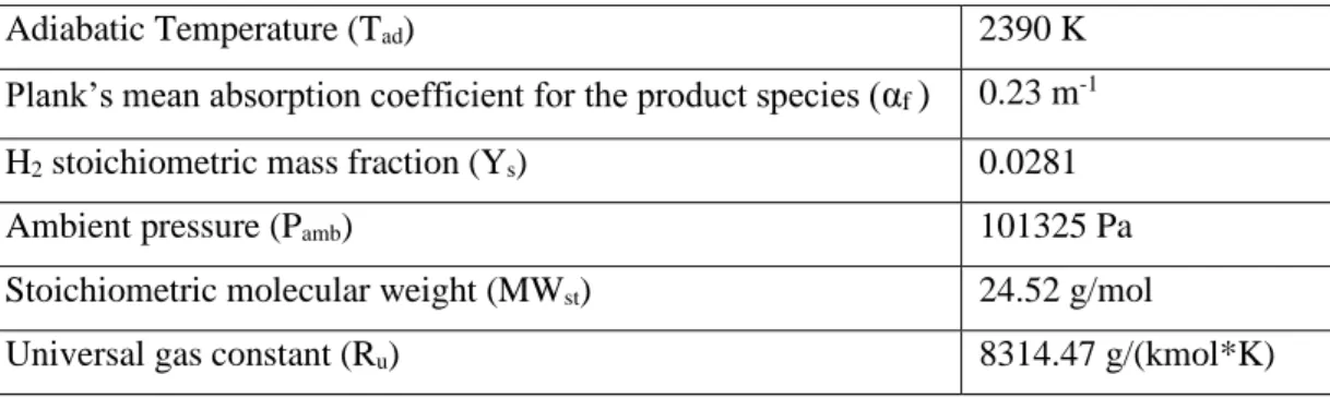
Table 3.13: Values used in the procedure for the heat flux predictions 57

Table 3.14: Classes of radiative heat flux (kW/m2) 60

(14)

xiv

Table 3.16: Threshold harm criteria of Thermal Doses required to give Pain, Burns and Fatal

Outcomes 64

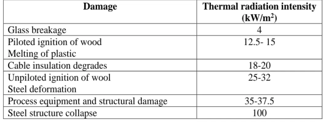
Table 3.17: Damage to structures and equipment due to thermal radiation for 30 min

expo-sure times 65

CHAPTER 4

Table 4.1: Pipeline operating parameters and source release properties employed in the

simulations 66

Table 4.2: Blast demand radius (m) at different levels of peak overpressure and impulse for

explosivity class 6 and atmospheric stability class D5 74

explosivity class 6 and atmospheric stability class F2 74

explosivity class 9 and atmospheric stability class D5 75

(15)

CHAPTER 1 Hydrogen

1.1 Introduction

In recent years, the increasingly massive depletion of energy resources and the gradual change in climatic conditions have become a topic of particular interest worldwide.

Incorrect use and exploitation of natural resources has led to their exhaustion. In reality, the progressive decrease in environmental resources is also linked to the increase in population: the great demographic growth leads to a decrease in the availability of resources.

Furthermore, the use of traditional fuels contributes to the increase in pollution, since it causes ever more greenhouse gas production. The more the concentration of these gases increases, the more the amount of heat in the atmosphere increases and, therefore, the tem-perature of our planet rises, making the survival of living species increasingly difficult. In order to overcome these problems, an effort to realize a gradual replacement of traditional fuels by alternative fuels, essentially represented by energy carriers, has been made.

Concerning its definition, an alternative fuel should have certain qualities.

First of all, it must be energy efficient, competitive from the economic point of view, toler-able from an environmental point of view, availtoler-able, cheap and safe (Balat, 2008).

In the scenario described above, hydrogen is considered one of the most promising fuels of the future, being convenient from an energy point of view, at low polluting impact and a renewable fuel.

Hydrogen is not a primary energy source existing in nature, but it must be produced; in other words, it is defined as an energy carrier.

Several production methods to produce hydrogen are known and they are related to both renewable and traditional energy sources.

Nowadays, the hydrogen production is based mostly on fossil fuels. Well-established tech-nologies (i.e. steam reforming of methane, partial oxidation of natural gas, coal gasification) are widespread, characterized by high efficiencies and low product costs. But innovative technologies based on renewable sources must be developed or improved so that hydrogen

(16)

can become more and more competitive. Alternative methods to produce hydrogen employ biomass, through pyrolysis/gasification processes, water, through electrolysis, direct thermal decomposition, thermochemical processes and photolysis (Baykara, 2018).

One of the major obstacles to the diffusion of hydrogen as an alternative fuel is related to the public perception of hydrogen as a “no-safe” fuel.

Certainly, hydrogen is not safer than the current energy sources (i.e. methane, gasoline), but it is not even more dangerous if compared to the other fuels. It must be handled accurately, taking in consideration its properties and the hazards that an inappropriate use can cause (Saffers and Molkov, 2014).

However, beyond the subjective "perception of risk", a careful analysis resizes the concept of hydrogen hazard.

In 2001 Swain (Swain, 2001) carried out the first comparison between a hydrogen and a gasoline fuel leak and ignition. As shown in Figure 1.1, the hydrogen-powered vehicle was undamaged, after both 3 s (left) and 60 s (right) from the fire initiation, on the contrary the gasoline-powered vehicle presented evident severe damage.

Figure 1.1: Hydrogen jet fire and gasoline fire

1.2 Hydrogen properties relevant to safety

Hydrogen is the most abundant element in the Universe. It is very rare in the Earth's atmos-phere, in which is present with a concentration of about 1 ppm and practically non-existent at pure state on the surface and in the subsoil of the Earth. It is present in combination with other elements.

(17)

First element of the periodic table, with an atomic number of 1.008 g/mol, hydrogen repre-sents the lightest founded element, consisting of one proton and one electron. Protium, deu-terium and tritium are the three isotopes of hydrogen. At its elementary state, it exists below diatomic molecule form (H2), whose atoms are held together by covalent bonds.

In atmospheric conditions and at room temperature (298 K), hydrogen is colourless, odour-less, tasteless and not detectable in any concentration by human sense. It is a highly flam-mable gas, non-corrosive and non-toxic.

In order to investigate the physical properties, the phase diagram of hydrogen, shown in Figure 1.2, is taken into consideration (Molkov, 2012).

Figure 1.2: The phase diagram of hydrogen

Hydrogen critical conditions are characterized by a temperature of 33.15 K and a pressure of 12.96 x 105 Pa. The point in which all three phases can coexist, called “triple point”, is represented by a temperature of 13.8 K and a pressure of 0.072 x 105 Pa.

At ambient pressure (1.01325 x 105 Pa), the boiling temperature is 20.37 K, which corre-sponds to a value of density of 70.90 kg/m3.

Hydrogen is characterized by a very low density (0.083 kg/m3) under normal conditions, and so it is stored at high pressure or cryo-compressed or as liquid, in order to increase its capac-ities. A high diffusivity (approximately 3 times that of the methane) characterizes the tiny molecules of hydrogen and its values are included in a range from 6.1 x 10-5 and 6.8 x 10-5 m2_/s.

(18)

The specific heat of gaseous hydrogen at constant pressure (cp) is 14.85 kJ/(kg K) in normal

conditions (NTP) and 14.304 kJ/(kg K) in standard conditions (STP). The specific heat ratio (γ) is 1.39 at NTP and 1.405 at STP (Molkov, 2012).

Hydrogen presents a thermal conductivity higher than the other gases: 0.187 W/(m K) at NTP and 0.01694 W/(m K) at STP.

At ambient conditions, the hydrogen reactivity is rather slow, but the presence of an activated agent, i.e. a catalyser or a spark, can accelerate the reaction and make it happen explosively. The main characteristic properties of hydrogen, which are taken into account in the aspects of use in safety, are the wide range of flammability, 4% to 75% by volume in air at STP, and the very low ignition energy. The minimum ignition energy for a stoichiometric hydrogen-air mixture is 0.018 mJ, 16 times lower than methane, and its autoignition temperature is 783 K.

The characteristic invisible flame of hydrogen can reach high values of temperature. For a stoichiometric mixture (constituted by 29.59 vol % hydrogen and 70.41 vol % air), the adi-abatic flame temperature is 2403 K (in air). Hydrogen has a heat of combustion higher than other fuels (119.93 MJ/kg) and a burning velocity ranging between 2.65 and 3.46 m/s, one order of magnitude larger than methane (Rigas and Amyotte, 2013).

Similarly to many real gases, hydrogen suffers an inverse Joule-Thompson effect. Following an expansion, its temperature increases; however, this increase in temperature is not nor-mally sufficient to ignite a hydrogen-air mixture. Further hazards may be considered when handling liquid hydrogen, because it evaporates easily.

The main hydrogen properties are summarized in Table 1.1.

Molecular weight (g/mol) 2.016

Density gas (kg/m3) liq (kg/m3)

0.0838 70.9

Boiling Temperature (at 1 atm) (K) 20.37

Freezing Temperature (K) 13.8 Critical point T (K) P (Pa) 33.15 12.96 x 105 Triple point T (K) P (Pa) 13.8 0.072 x 105

(19)

Diffusivity (m2_/s) _{6.1 x 10}-5

Stoichiometric mixture (% vol) 29.59

Ignition energy (mJ) 0.018

Flammability range (in air) (% vol) 4 -75

Adiabatic flame Temperature (K) 2403

Autoignition Temperature (K) 783

Latent heat of vaporization (kJ/kg) 445.6

Table 1.1: Main hydrogen properties

Another property of hydrogen which must be taken into consideration in a safety assessment is the buoyancy.

On Earth, hydrogen is the element with the highest buoyancy, being its density lower than that of the air and so it is inclined to not accumulate in the atmosphere, but rapidly to disperse. Above a temperature of 22 K, pure hydrogen presents positively buoyant.

The hydrogen dispersion is more influenced by the buoyancy than by the diffusivity. As a consequence, a hydrogen release is diluted quickly in the air and its concentration falls out of the flammability range.

The buoyancy effects in unintended hydrogen releases must be taken into account in the evaluation of the type of jet generated. Based on this effect, three types of jets can be identified: momentum-dominant jets, buoyancy-dominant jets and transitional jets, as shown in Figure 1.3 for a horizontal jet (Molkov, 2012).

Figure 1.3: Momentum-controlled jet, transitional jet and buoyancy-controlled jet for a horizontal

(20)

1.3 Hazards related to the use of hydrogen

Hazard can be defined as “a chemical or physical condition that has the potential for causing

damage to people, property and the environment” (Molkov, 2012).

Regarding the impact on the environment, since the hydrogen exists naturally in the atmosphere, it does not contribute to alter the environmental stability; the hydrogen gas will be dissipated rapidly in air. When used as a fuel, it does not generate fumes or smoke and, above all, its combustion does not produce greenhouse gases, so hydrogen will not contribute to the atmospheric pollution.

Moreover, hydrogen will not play a part in the groundwater contamination, being a gas at normal atmospheric conditions (HyResponse Report, 2016 (a)).

On the contrary, the impact of hydrogen on people and property is different.

Hydrogen is not considered a carcinogen and no cases of mutagenicity, embryotoxicity, teratogenicity or reproductive toxicity have been shown at present. Hydrogen should not be ingested and, if inhaled, can create a flammable mixture within the human’s lungs. It is defined as a simple asphyxiating gas, since a reduction in oxygen concentration in air due to hydrogen may cause breathing problems (dyspnoea). Symptoms as headaches, dizziness, unconsciousness, nausea, vomiting can be present in individual exposition or breathing these atmospheres. Liquid hydrogen can cause hypothermia, also.

In addition to the harms related to people exposure in an area in which an accidental release of hydrogen has occurred, the other harmful effects due to hydrogen combustion have to be considered.

Direct contact with hydrogen flames and radiant heat flux from hydrogen fires, and overpressure and impulse following an explosion are the main harms at which people and property are exposed.

1.4 Thesis objectives

The aim of this thesis is the assessment of damage to people and buildings following a hydrogen pipeline failure.

First of all, a historical analysis of accidents involving hydrogen has been carried out, in order to define the main causes and the related consequences. Mechanical failure of

(21)

components of facilities, pipelines or tanks is considered the most common source of accidents.

The first objective is to investigate the potential scenarios connected with a rupture of pipelines transporting gaseous hydrogen. An uncontrollable leakage of gas will mix with air and create a flammable cloud. If a source of ignition is present, a fire or an explosion can occur.

The second objective is the evaluation of the consequences of a jet fire and an explosion on people and properties in the proximity of the accidental event. In the case of a fire, the main hazard to humans and surroundings is connected with the heat radiation, in the case of an explosion the main hazard is related to the overpressure and the impulse generated.

In order to establish the probability that an explosion and a jet fires can cause a given effect, a probabilistic risk assessment procedure for the estimation of damage on two types of buildings (i.e. reinforced concrete and tuff stone masonry buildings) and on people involved in the accident has been proposed.

SLAB one-dimensional integral model has been used to evaluate the atmospheric dispersion of gaseous hydrogen release and, in order to characterize the jet release and the flammable cloud size, a release rate model has been incorporated in this dispersion model.

The overpressure and the impulse resulting from the explosion were estimated through the Multi-Energy Method. Pressure-impulse diagrams has been used to assess the damage to the building structures.

SLAB model has been employed to evaluate the flame length: the distance at which a hydrogen concentration corresponding to the limit lower flammability (4%) has been considered. Empirical correlations of literature have been applied to determine the radiative heat flux. The point source model has been employed to estimate the radiative heat flux with the radiant fraction calculated through the correlation proposed by Molina et al. (2007). In order to ensure their applicability, a validation against experimental data has been carried out.

Finally, damage to people involved in the failure of gaseous hydrogen pipelines were estimated through the Probit functions, which causative variables are represented by the key parameters of the two accidental events considered, overpressure and impulse in the case of the explosions and radiative heat flux in the jet fires one.

(22)

Several parameters related to the pipeline characteristics (i.e. pipeline diameter, operating conditions), source release properties (i.e. hole diameter, length of the pipeline from the compression stations) and the atmospheric conditions were taken into consideration to assess the hazards connected with the pipeline failure.

Finally, a minimum safety distance between hydrogen pipelines and people and buildings has been estimated and the procedure proposed can be a useful tool in the design of future pipeline networks and in the assessment of the existing ones.

1.5 Thesis structure

The thesis is structured in five chapters.

In the first chapter a brief overview on the hydrogen potential capabilities as an energy carrier is given, investigating on its physical and combustion properties and the hazards related to an inappropriate handling.

In chapter two, the main methods of delivering hydrogen to the point of use are described. From the performed analysis, it resulted that the most efficient method to transport large quantities of hydrogen is via pipeline. The potential risks connected to failure of a hydrogen gaseous pipeline has been investigated to preserve the health of the people and the integrity of properties in the environment surrounding the area of the accidental event. The potential scenarios have been delineated, also. Fires and explosions were identified as the most fre-quent events that can occur. A probabilistic procedure to assess the risks connected to jet fires and explosions involving a rupture of a pipeline carrying gaseous hydrogen has been proposed.

Chapter three describes the consequence of a pipeline failure and the effects that it can cause. Both damage to different types of buildings and to people have been taken into consideration. In order to characterize the accidental events that can occur and the quantities that represent them, the dispersion and explosion models and the radiation procedure used in this work have been preliminarily analysed and validated against experimental data.

Chapter four presents the results obtained from the performed analysis, in terms of probability of damage and minimum safety distance.

(23)

CHAPTER 2 Hydrogen accidents

2.1 Introduction

In order to be considered a successful energy carrier, hydrogen must be economically competitive and the individual technological components must be connected through an infrastructure that provides a safe and environmentally friendly energy system throughout production, from distribution to final use.

The hydrogen market involves two segments: “merchant hydrogen” and “captive hydrogen”. The term “merchant” refers to hydrogen generated in a central production plants and provided to consumers through a pipeline network, tanks or truck delivery; instead, the terms “captive” specifies hydrogen produced directly on the point of use. Currently, the hydrogen market is dominated by the captive hydrogen, which covers 95% of it and it is presumed that it will continue to control it until 2021. In any case, lately, the merchant hydrogen market is expanding and in the USA it has reached about 7% per year. North America represents the widest market for merchant hydrogen (Bezdek, 2019).

Hydrogen production plants are located all over the World, as shown in Figure 2.1 (h2tools database, 2019).

Figure 2.1: Hydrogen Production Plant Distribution in the World

Nowadays, hydrogen is used in many types of industries and for different processes. Most of all, the hydrogen produced is employed in the chemical industry to produce ammonia,

(24)

methyl alcohol, fertilizers for agriculture and petroleum products, and in the metallurgical industry for metal treatment. Furthermore, hydrogen is an excellent fuel that can be used to produce energy, in burning hydrogen alone or added to other fuels or directly obtaining electrical energy through a fuel cell. In Figure 2.2 the capacity (Nm3/h) of the various hydrogen plants diffuse in the World is illustrated (h2tools database, 2019). Data were updated in January 2016 and are related to existing and operating medium and large plants. Many companies have invested in this market and these investments are destined to grow. A recent agreement has been stipulated between the Linde Group and the Praxair Inc, to supply a hydrogen plant in Louisiana, with a production capacity of over 190,000 Nm3/hr, coming on stream in 2021 (Linde Engineering News, 2019).

Figure 2.2: Capacity (Nm3_{/h) of hydrogen production plants}

In recent years, also Europe has been interested in this market and the investments have been increasingly substantial, as shown in Table 2.1 (Eurostat, accessed on 2019).

2010 2011 2012 2013 2014

Million Nm3 _17.799 _17.961 _18.345 _18.240 _18.633

(25)

Generally, hydrogen production plants are located in large industrial sites; consequentlythe hydrogen produced, regardless of the method used, must be transported from the point of production to the point of utilization (Jo and Ahn, 2006). The hydrogen distribution infrastructure needed for distributing hydrogen to the nationwide network must be increasingly developed.

Hydrogen delivery can be carried out through transmission and distribution lines. The former deliver hydrogen from a production plant to a single point, the latter from a production plant to a distributed network of refuelling stations located in a city or a region.

Currently, the means of transportation which are used in the hydrogen distribution are: pressed tube trailers, cryogenic liquid trucks and compressed gas pipelines. Since the com-pressed tube trailers cannot handle large capacities of gas (~300 kg of hydrogen), they can be employed only at small scales and used primary for distances of 200 miles or less, and hence they are inefficient from an energetic point of view to meet market demands. Higher volumes can be carried by cryogenic liquid trucks (~ 400-4000 kg of liquid hydrogen), but the high cost and high energy use in the liquefaction process represent the main disad-vantages in the use of this kind of delivery (Balat, 2008).

Compressed gas pipelines are the most suitable options to transport large quantities of hy-drogen, for high efficiency and low costs.

The major companies have built hydrogen pipeline networks to ensure a stable and uninter-rupted hydrogen supply, as shown in Table 2.2 (h2tools database, 2019).

USA have got the largest hydrogen pipeline network, with 2608 km, followed by Europe with 1598 km. Hydrogen pipelines Company km Miles Air Liquid 1936 1203 Air Product 1140 708 Linde 244 152 Praxair 739 459 Others 483 300 Word total 4542 2823

(26)

Pipelines are usually located in industrial areas, but they can also be found in rural and pop-ulated zones (Zhang, 2018). For example, in Europe, from Rotterdam to Dunkerque, via Antwerp, a hydrogen pipeline network extends for 900 km.

In view of this, the potential risks due to a failure of a hydrogen gaseous pipeline must be investigated to preserve the health of the people and the integrity of properties in the envi-ronment surrounding the area of the accidental event.

2.2 Elements of risk analysis

According to the AIChE/CCPS (2000), Risk is “a measure of human injury, environmental damage or economic loss in terms of both the incident likelihood and the magnitude of the loss or injury” (Crowl and Jo, 2011). The combination of a risk analysis and a risk evaluation is called risk assessment.

In order to perform a correct risk assessment, hazards must be identified, possible accident scenario delineated, acceptance criteria specified and the consequences evaluated.

Several methodologies to perform a risk assessment have been reported in literature and applied in different fields. For example, recently, a quantitative risk assessment on a hydrogen refuelling station has been performed (La Chance et al., 2009, Russo et al., 2018). The risks associated with hydrogen transportation across cities and the countryside by pipelines or tube trailers are investigated in a study carried out by Gerboni and Salvador (2009). Historical analysis of hydrogen accidents is a useful tool to identify the possible hazards and establish the main causes and consequences related to an accidental event. Several types of accidents have been identified. Generally, six causes are considered the most frequent: i) third parties operations, that are related to activities or interferences caused by others in the proximity of pipelines and not due to an inaccurate management; ii) corrosion, related both to the feature of the transported materials and to the pipe coating; iii) mechanical failure, related to the cracks that occur when the system is subjected to excessive stresses with respect to those the system permits; iv) operational errors, which are caused by an incorrect system management; v) natural events, such as floods, earthquakes, frost; vi) other or unknown causes (Papadakis, 1999).

Various databases were generated in order to collect incidents and to learn from the past. MHIDAS (Major Hazard Incident Accident Data Service) database contains data related to hazardous materials accidents. It reports that the mechanical failure is the most recurrent

(27)

cause of an accident involving hydrogen, analysing a total of 118 accidents (1934-2009), as illustrated in Figure 2.3 (Gerboni and Salvador, 2009).

Figure 2.3: Main causes of accidents involving hydrogen (data from Gerboni and Salvator, 2009)

Data has been confirmed by HIAD (Hydrogen Incident and Accident Database), that collects almost 300 hydrogen events, accidents, incidents and near misses (HIAD database, accessed on April 2019). In addition, HIAD presents different sections, depending on the hydrogen system of interest (industry, laboratories, transport).

Valves, flanges, pumps and compressors are some of the components most subjected to mechanical failures, and, since they are additional elements to the main body of the pipeline, an assessment of events involving a failure of hydrogen transportation entails such components to be accounted for.

Due to its low viscosity, hydrogen is much more predisposed to leakages from piping connections than hydrocarbons (HYPER, 2008).

An accurate incidents analysis gives information both about frequency of the initiating event and about the consequences of event (Mirza, 2011).

Investigating on several incidents involving hydrogen pipeline, the probability of pipeline rupture has been evaluated, highlighting that the failure can resolve in a full bore rupture or in a small/partial leak. Air Liquide (2005) has estimated the probability of pipeline rupture in year per km of length of pipeline, as shown in Table 2.3.

(28)

Table 2.3: Probability of pipeline rupture (source: Air Liquide, 2005)

The following step of the assessment was to analyse the consequences of an accidental pipeline failure carrying gaseous hydrogen. This type of event can lead to various outcomes. A useful tool to delineate the potential accident scenarios is represented by the event tree analysis. An example of an event tree related to a pipeline accident is reported in Figure 2.4. As shown, hydrogen atmospheric dispersion is the scenario that occurs with a major frequency, but following this event no significant harmful consequences are found.

The next question for an event tree is the probability of ignition. An accurate analysis discerns the ignition into two categories: immediate and delayed, because the consequences that this may cause are different. If an immediate ignition occurs, jet fires is the unique accident that takes place. At a delayed ignition, instead, a hydrogen cloud may form and successively explode. The probability that one of two above-mentioned events takes place will depend on the different features of the surrounding environment (open, confined, ventilated) and on the degree to which it mixes with the air, as well as the power of ignition source.

* data from Air Liquide: probability of pipeline rupture [year x km] of 2 x 10-5, assuming a pipeline length of 25 km;

** data from OREDA (Sintef Technology and Society. Offshore reliability data handbook. In: OREDA 2002. 4th_{ed. Høvik, Norway;}

*** data from the statistic report: Available at: http://www.ntsb.gov/publictn/2002/HZM0202.pdf

Figure 2.4: Example of an event tree constructed for a failure of a pipeline carrying hydrogen

(29)

The frequency of occurrence of explosions and jet fires are 1.34 x 10-5_{/year and 5.00 x 10}-6

/year, respectively, as reported by Gerboni and Salvator (2009).

Finally, it is important to quantify the damage and the consequences for people and property in the surrounding area.

The major damage related to the accidental scenarios described above is the collapse of buildings under explosions, and both direct and indirect effects of blast and thermal radiation on people.

In the case of an explosion, local damage to structural elements of buildings, exposed to severe overpressure, can result in a progressive collapse of the whole structure.

In the case of fires, structural components are less affected by smoke and temperature.

2.3 Methodology

In order to estimate the damage to people and buildings involved in an explosion or in a fire due to a high-pressure hydrogen pipeline failure, in this work a probabilistic risk assessment procedure is proposed.

Several probabilistic risk assessment methodologies are proposed in literature. One of the most used is based on the Bayesian Belief Networks (BBN); it is applied to predict the structural stability of civil structures and in process industries.

Risk analysis framework, suggested by Ellingwood (2006), and reported by Russo and Parisi (2016), permits to estimate the annual probability of a structural collapse C caused by an extreme event H, as a combination of the conditional probability of the event of progressive collapse given the local damage (LD) event occurs (Pr[C|LD]) and the conditional probability of local damage given the extreme event H (PR[LD|H]), multiplied by the mean annual rate of occurrence of H (λH) (Equation 2.1):

Pr[𝐶] = Pr[𝐶|𝐿𝐷] Pr[𝐿𝐷|𝐻] 𝜆𝐻 (2.1)

Then, the evaluation of the probability of a progressive collapse can be estimated using the following equation:

Pr[𝐶] = Pr[𝐶|𝐿𝐷] Pr [𝐿𝐷] (2.2)

In the case of an explosion, caused by an accidental release of hydrogen, the annual probability of local structural damage is evaluated as follows:

Pr[𝐿𝐷] = Pr[𝐿𝐷|𝐸] Pr [𝐸|𝑅] 𝜆𝑅 (2.3)

where E is the explosion event, R is the pipeline rupture, λR is the annual mean rate of

(30)

The terms Pr[LD|E] and Pr[E|R] indicate the conditional probability of the local damage given the extreme event E and the conditional probability of extreme event E given R, respectively.

Pr[E|R] represents the blast hazard function that provides the probability of occurrence of the explosion as a consequence of the pipeline rupture. Pr[LD|E] represents the blast fragility of the structural components.

Multi-Energy Method is used to calculate the blast hazard.

This approach is then extended to the evaluation of the annual probability of damage to people subjected to an extreme event (i.e. explosion, jet fire), following a failure of a hydrogen pipeline, through the Equation 2.4:

𝑃𝑟[𝐷] = 𝑃𝑟[𝐷|𝐸]𝑃𝑟[𝐸|𝑅]𝜆𝑅 (2.4)

where D is the damage to people; E is the accidental event; R is the pipeline rupture; λR is

annual rate of pipeline rupture occurrence, in a year per 1,000 km. Probit equations are employed to calculate the damage probability.

(31)

CHAPTER 3 Consequences of accidents involving gaseous hydrogen

3.1 Introduction

Pipeline carrying gaseous substances, following an accidental event can result in full rupture or in a hole in the pipe and can cause a release of a large quantity of gas, with consequent diffusion and formation of a cloud.

In order to assess the consequences that can derive from it, after identifying the accident, a release model is developed to describe how the material was released and, subsequently, the concentrations of the released material are estimated by dispersion models.

Finally, the effects that the failure can cause in the surrounding environment are evaluated. Release models (or source models) are a useful tool to calculate the amount of substance released. These models are built upon basic equations or empirical relationships, that represent the chemical-physical phenomena occurring during the release.

3.2 Hydrogen release through a hole

Gaseous hydrogen discharges through a hole in a pipe can be described taking into account the free expansion release source models, as shown in Figure 3.1 (Crowl and Louvar, 2011). When a high-pressure gas flows and expands through a hole, its pressure energy is converted to kinetic energy.

The released gas flow is obtained solving a mechanical energy balance, considering that density, temperature and pressure are not constant, but they vary considerably between upstream and downstream. An isentropic transformation is assumed.

(32)

During the expansion, the gas velocity changes with time. The maximum flow rate is found at the hole, where the higher value of downstream pressure is reached. This pressure is called choked pressure (Pchoked) and is evaluated through the following Equation:

𝑃𝑐ℎ𝑜𝑘𝑒𝑑 𝑃0 = ( 2 𝛾+1) 𝛾 𝛾−1 (3.1)

where Po is the pressure in the initial condition and γ is the ratio of the heat capacities at

pressure and volume constant (γ=Cp/Cv). In these conditions, the velocity of the gas at the

hole is the velocity of sound. These assumptions allow to define a peak initial release, calculated with Equation 3.2:

𝑄_{𝑝𝑒𝑎𝑘} =𝜋 𝑑₄2 𝛼 √𝛾 𝜌0 𝑃0 (_𝛾+12 )

𝛾+1 𝛾−1

(3.2)

assuming that α is the ratio of effective hole area to the pipe sectional area (dimensionless hole size), d is the pipe diameter, ρ0 and P0 are the stagnation density and pressure of gas at

initial conditions, respectively, and γ is the specific heat ratio of gas.

After reaching the initial peak, the release rate decays over time until it achieves a steady-state; Equation 3.3 allows to obtain this value:

𝑄_{𝑠𝑡𝑒𝑎𝑑𝑦−𝑠𝑡𝑎𝑡𝑒} = 𝑄𝑝𝑒𝑎𝑘 √1+(4 𝛼2_𝑓_𝐹𝐿 𝑑)( 2 𝛾+1) 2 𝛾−1 (3.3)

where fF is the Fanning frictionfactor and L is the pipe length from the hydrogen supply

station to the release point.

The correlation of Nikuradse has been adopted to value the Fanning frictionfactor, as pro-posed by Molkov (2012):

1

√𝑓𝐹 = 0.869 ln(𝑅𝑒 √𝑓𝐹) − 0.8 (3.4)

A value of 0.005643 for fF has been obtained.

Overestimated values of the mass flow rate of the discharged mass, applied for a gaseous hydrogen release through high pressure pipe, were noted.

A study of the physical properties of the gaseous hydrogen stored at high pressures showed a different behaviour of this gas compared to ideal gases. In order to describe the character-istics of real gas, the Abel-Noble equation of state (Equation 3.5) is taken into account and

(33)

incorporated in the Equation 3.2, for the computation of ρ0. This equation permits to evaluate

the compressibility factor z, expressed in terms of co-volume (b): 𝑧 = 1 + 𝑏 𝜌0

𝑅𝐻2 𝑇 (3.5)

where b is 7.69 10-3 m3/kg, RH2 isthe hydrogen gas constant, i.e. the ratio of the universal

gas constant R to the molecular mass of hydrogen (4124.24 J/kg/K).

3.3 Hydrogen dispersion

Gaseous hydrogen, leaking from a pipeline involved in an accidental event, diffuses into the surrounding environment and various outcomes can arise, depending on the conditions in which the spill occurs.

Several dispersion models are present in the literature to describe the ways in which the gas disperses away from the discharge point and to estimate the downwind concentrations of the released gas. The dispersion calculations also permit to define the area involved in the event (Crowl and Louvar, 2011).

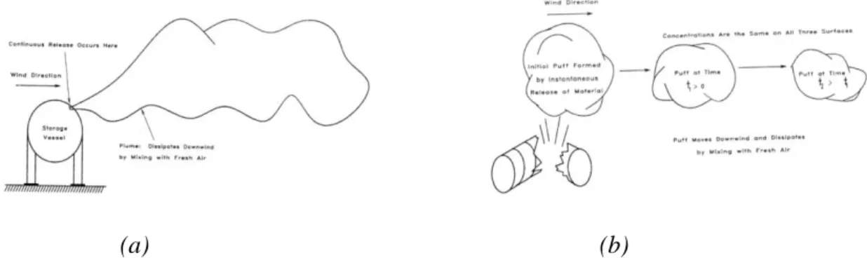
Depending on the duration of the release, continuous or instantaneous, a characteristic plume or puff can be generated, respectively, as shown in Figure 3.2 (a) and (b).

(a) (b)

Figure 3.2: Characteristic plume following a continuous gas release (a) and puff following an

instantaneous gas release (b).

As the gas moves away from the point of release, where the concentration is maximum, it is diluted due to turbulence phenomena and dispersion in air and therefore its concentration is lower.

Several parameters can affect the dispersion and allow a different process evolution. These parameters are essentially characteristic of the environment in which the release takes place,

(34)

as the wind speed, the atmospheric stability, the ground conditions, the height of the release above ground level, the momentum and the buoyancy of the gas released.

The meteorological conditions influence the dispersion of the gas in the atmosphere, so a careful evaluation is necessary in order to optimally define the development of the event. In fact, a high wind speed value allows a greater dispersion of the gas, being diluted faster by a greater quantity of air. Atmospheric stability tends to be classified according to three main classes: stable, neutral and unstable. Pasquill et al. (1961) have established six stability classes, identified with letters A (the least stable conditions) to F (the most stable one), as reported in Table 3.1:

Table 3.1: Meteorological condition by Pasquill-Guifford stability classes

The wind speed and the quantity of sunlight are taken into consideration in the definition of these stability classes.

Furthermore, the ground characteristics contribute to improving or worsening the phenomenon of dispersion, since it is possible to create mechanical mixing on the surface; the presence of trees and buildings increases mixing, while open areas make it decrease. Initially, the dispersion is influenced by the speed of the discharge and therefore the momentum will prevail. Departing from the discharge point, the buoyancy comes into play; the denser fluids of the air will tend to fall back to the ground, while the lighter ones will remain suspended. The fundamental parameter is therefore density, on the basis of which a general subdivision can be made between compounds released in heavy gases (density greater than air), neutral gases (same density) and light gases (lower density).

(35)

3.3.1 The SLAB model and its validation for hydrogen dispersion

The models used to describe the dispersion phenomenon in the atmosphere can be classified into two families: integral models and three-dimensional models. The integral models solve the mass, energy and momentum balances in simplified forms in order to obtain equations of simple numerical integration; in this way, more determining factors can be taken into account in the economy of the dispersive phenomenon, above all the buoyancy phenomena, but the integral models do not yet allow the modelling of complex geometries.

Three-dimensional models are exploited by computational fluid dynamics (CFD). As the previous ones, they numerically integrate the fundamental balances, but they are able to be applied to any type of fluid in any geometry, even very complex. Furthermore, these models take into consideration turbulence models, but their weaknesses are the high costs and the long calculation times. On the contrary, the integral models require lower costs and relatively low computational times.

In this work, the modelling of the dispersion phenomenon has been performed using the one-dimensional integral model SLAB developed by Lawrence Livermore National Laboratory (Ermark, 1990).

SLAB is a computer model that simulates the jet evolution of a release and its dispersion in the atmosphere. Various types of releases can be considered, e.g. a ground-level evaporating pool, an elevated horizontal or vertical jet and an instantaneous volume source.

The conservation equations of mass, momentum, energy and species are employed to evaluate the atmospheric dispersion of the release. Three steps are planned in the simulation: source identification and initialization of the event of dispersion, valuation of cloud dispersion and valuation of the time-averaged concentration.

Depending on the source type and the loss duration, both modes of atmospheric dispersion, i.e. steady state plume and transient puff mode, are taken into consideration. Figure 3.3 shows the cloud dispersion for heavy gas in the plume dispersion mode, reproduced by SLAB.

(36)

Figure 3.3: Dispersion cloud in the plume dispersion model by SLAB

Several information is required to obtain a correct and fairly complete simulation that describes how the phenomenon of dispersion develops. Data concerning source, spill, field and meteorological properties are used as input parameters and employed to describe the generating cloud.

The most significant output of the simulation is the time-averaged concentration, expressed as the time-averaged volume fraction, as shown in Equation 3.6:

𝐶(𝑥, 𝑦, 𝑧, 𝑡) = 𝐶𝐶(𝑥) × ⌈erf(𝑥_𝐴) − erf (𝑥𝐵)⌉ × [erf(𝑦𝐴) − erf(𝑦𝐵)] × [exp(−𝑧𝐴2) + exp(−𝑧𝐵2)] (3.6) assuming the following expression for the terms presents in the previous equation: 𝑥𝐴 = (𝑥 − 𝑥𝑐+ 𝑏𝑥) (√2⁄ × 𝛽𝑥) 𝑥𝐵 = (𝑥 − 𝑥𝑐− 𝑏𝑥) (√2⁄ × 𝛽𝑥) 𝑦_𝐴 = (𝑦 + 𝑏) (√2⁄ × 𝛽_𝐶) 𝑦_𝐵 = (𝑦 − 𝑏) (√2⁄ × 𝛽_𝐶) 𝑧_𝐴 = (𝑧 − 𝑧_𝐶) (√2⁄ × 𝑠𝑖𝑔) 𝑧𝐵 = (𝑧 + 𝑧𝐶) (√2⁄ × 𝑠𝑖𝑔)

in which erf and exp are the error and the exponential function, respectively; x, y and z are the coordinates of the reference system; zc is the profile centre height (m), bx is the

half-length parameter (m), b is the half-width parameter (m). 𝛽_𝐶, 𝛽_𝑥 and sig are parameters listed in the output.

(37)

It was assumed that the concentration profiles have a Gaussian shape and are evaluated in the downwind direction. A weakness of this model is that is does not consider the gas flow around obstacles and does not take into account complex terrain.

The SLAB model is usually employed to simulate dispersion of heavy gas. In order to apply it in the case of hydrogen dispersion, a validation against available experimental data in literature has been realized.

Shirvill et al. (2006) have investigated hydrogen dispersion experiments carried out by Shell Global Solutions and the Health and Safety Laboratory (HSL) to describe the jet releases of hydrogen.

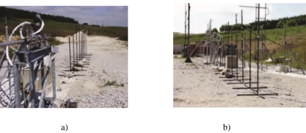
The experimental tests consisted of controlled releases of hydrogen, realized at pressures varying between 1 and 15 MPa. The Figure 3.4 (a) and (b) show the test facility; gaseous hydrogen was released horizontally through different orifices (1, 3, 4, 6 and 12 mm), located at 1.5 m above the ground.

a) b)

Figure 3.4: Experimental setup related to the trials of Shirvill et al (2006)

Oxygen concentration measurements within the generated cloud were carried out to assess the hydrogen concentration. The following relationship has been used:

𝐶_𝐻₂= 100% × (𝑉₀− 𝑉_𝑚)/𝑉₀ (3.7) where: V0 is the sensor output in air and Vm is the sensor voltage in a reduced-oxygen

atmosphere. 13 CiTicel AO2 Oxygen sensors, located at different distances from the nozzle, were employed to observe oxygen concentration. Measurements of wind speed and direction were performed.

(38)

Run Pressure [MPa] Temperature [°C] Leak diameter [mm] 1 12 20 4 2 13 18 4 3 12.6 17 4 4 13.7 17 3 5 12.3 15 3 6 11.9 15 3 7 10 14 3 8 9.9 14 3 9 9.3 13.5 4 10 9.4 13 4 11 7.7 13 4 12 7.4 14 3 13 7.4 13.5 3 14 5.0 12.5 3 15 5.6 13 3 16 5.1 14.5 4 17 5.4 14.5 4 18 4.3 14 6 19 4.1 14 6 20 2.3 13.5 6 21 2.6 14 4 22 2.5 14.5 3 23 1.1 14.5 12

Table 3.2: Experimental conditions related to the trials of Shirvill et al. (2006)

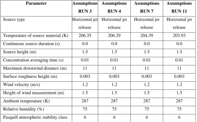
Simulations were carried out to validate the SLAB model. SLAB Simulations conditions for the run 3, 4, 7, 11 are reported in Table 3.3.

Parameter Assumptions RUN 3 Assumptions RUN 4 Assumptions RUN 7 Assumptions RUN 11

Source type Horizontal jet release Horizontal jet release Horizontal jet release Horizontal jet release Temperature of source material (K) 206.35 206.29 204.39 203.93

Continuous source duration (s) 0.0 0.0 0.0 0.0

Source height (m) 1.5 1.5 1.5 1.5

Concentration averaging time (s) 0.01 0.01 0.01 0.01

Maximum downwind distance (m) 11 11 11 11

Surface roughness height (m) 0.003 0.003 0.003 0.003

Wind velocity (m/s) 1.2 1.2 1.2 1.2

Height of wind measurement (m) 1.5 1.5 1.5 1.5

Ambient temperature (K) 287 287 287 287

Relative humidity (%) 75 75 75 75

Pasquill atmospheric stability class 6 6 6 6

(39)

Comparisons between experimental data and simulation results in terms of centreline hydrogen concentration decay as a function of distance are reported in Figures 3.5, 3.6, 3.7 and 3.8 for run 3, 4, 7 and 11, respectively.

Figure 3.5: Comparison of hydrogen concentration (expressed in terms of volume fractions) vs distance between SLAB predictions and experimental data by Shirvill et al. (2006) in the

conditions of RUN 3.

Figure 3.6: Comparison of hydrogen concentration (expressed in terms of volume fractions) vs

distance between SLAB predictions and experimental data by Shirvill et al. (2006) in the conditions of RUN 4.

e= 39%

(40)

A reasonable agreement between predictions and experiments has been shown in most cases considered. The prediction of the relative error (e), calculated through the Equation 3.8, has been evaluated.

(41)

𝑒 =_𝑁100

𝑒𝑥𝑝∑ |𝐶𝐻2−𝑝𝑟𝑒𝑑− 𝐶𝐻2−𝑒𝑥𝑝|/𝐶𝐻2−𝑒𝑥𝑝

𝑁𝑒𝑥𝑝

𝑖=1, (3.8)

As reported by the graphs, it is noted that the relative error is 39% for the Run 3, 22% for the Run 4, 52 % for the Run 7 and 49% for the Run 11. The data disagreement is due to the fact that the jet is affected by a crosswind during the experimental tests.

Another set of data used in the model validation are related to the experimental trials conducted by Han et al. (2014) to investigate the behaviour of high-pressure gaseous hydrogen released through small orifices.

The experimental setup, reported in Figure 3.9, consisted of a vessel containing hydrogen, on top of which a release hole was located. Three different hole diameters (0.5, 0.7 and 1 mm) were chosen and value of 100, 200, 300 and 400 bar have been taken into account as release pressure.

Figure 3.9: Experimental setup considered by Han et al. (2014)

To analyse the dispersion characteristics, the hydrogen concentration was detected along the jet centreline, considered horizontal. A Nd-YAG laser sheet was used to visualize the hydrogen jet. The experimental conditions are summarized in Table 3.4.

Case Pressure [bar] Leak diameter [mm]

1 100 1 2 100 0.7 3 100 0.5 4 200 1 5 200 0.7 6 200 0.5 7 300 1 8 300 0.7 9 300 0.5 10 400 1 11 400 0.7

(42)

SLAB simulations conditions are reported in Table 3.3.

Parameter Assumptions

Source type Horizontal jet release Temperature of source material (K) 206 K Continuous source duration (s) 12

Source height (m) 1

Concentration averaging time (s) 0.01 Maximum downwind distance (m) 10 Surface roughness height (m) 0.003

Wind velocity (m/s) 2

Height of wind measurement (m) 1

Ambient temperature (K) 288

Relative humidity (%) 75

Pasquill atmospheric stability class 6

Table 3.5: SLAB simulation parameters for experiments by Han et al. (2014)

The comparisons of centreline hydrogen concentration decay as a function of distance are shown in Figure 3.10, 3.11 and 3.12 for a pressure release of 100, 200 and 300 bar, respectively, in the case of a leak diameter of 1 mm.

distance between SLAB predictions and experimental data by Han et al (2014) (P= 100 bar, dh=1 mm).

(43)

distance between SLAB predictions and experimental data by Han et al. (2014) (P= 200 bar, dh=1 mm).

distance between SLAB predictions and experimental data by Han et al. (2014) (P= 300 bar, dh=1 mm).

SLAB model predicts optimally experimental data in the conditions considered, summarized in Table 3.5. The fairly low values of the relative errors estimated (25%, 13% and 16%, related to a dhole of 1 cm and pressure of 100, 200 and 300 bar, respectively) confirm this

trend.

(44)

Therefore, the small discrepancies between the experimental measurements and the predictions could be due only to the viscous dissipation of the flow passing through a small hole.

Okabayashy et al. (2005) have carried out experimental tests to estimate the dispersion concentration range following a leakage involving hydrogen refuelling stations. Five high-pressure tanks, with a total volume of 2500 L, and containing gaseous hydrogen stored at 65 MPa and released to 40 MPa were used to perform the trials. Leakage from hole with diameter varying between 0.25 mm and 2 mm were analysed. Measurements of concentrations along the jet have been realized, considering stable wind conditions (1 m/s), and eight sensors located at different distances from the hole were employed.

Table 3.6 summarizes the SLAB conditions used in the simulations.

Parameter Assumptions

Source type Horizontal jet release Temperature of source material (K) 205.34 K Continuous source duration (s) 1

Source height (m) 1

Concentration averaging time (s) 0.01 Maximum downwind distance (m) 20 Surface roughness height (m) 0.003

Wind velocity (m/s) 0.2

Height of wind measurement (m) 1

Ambient temperature (K) 288

Relative humidity (%) 75

Pasquill atmospheric stability class 6

Table 3.6: SLAB simulation parameters for experiments by Okabayasky et al. (2005).

The comparison between simulated data and experimental data in the case of df= 2 mm and

P=200 bar, is reported in Figure 3.13. As shown, simulation results reproduce experimental data reasonably, with a relative error of 28 %.

(45)

distance between SLAB predictions and experimental data related to Okabayashy et al. (2005).

This reproducibility of the data can also be seen in the simulations made in the other cases considered, whose simulation conditions are summarized in Table 3.6:

Finally, all the experimental results obtained were collected and reported in the Figure 3.14.

Figure 3.14: Predicted values of hydrogen concentration vs experimental values of hydrogen