The cosmic rays flux from the Pierre Auger Observatory data

Universit`

a degli Studi di Roma

“Tor Vergata”

Facolt`a di Scienze Matematiche, Fisiche e Naturali Dipartimento di Fisica

Dottorato di Ricerca in Fisica XXI ciclo

PhD Thesis

The cosmic rays flux from the Pierre

Auger Observatory data

Candidato : Claudio Di Giulio

A.A. 2008/2009

Relatore : Prof. Giorgio Matthiae

Acknowledgments

I would like to thank Prof. Giorgio Matthiae and Valerio Verzi for believing in me and for all the support they gave me. I would also like to thank Paolo Privitera, Paolo Petrinca and Pedro Facal for all I learned from them. A special thank at Mar´ıa Monasor, Mat´ıas Tueros and Gonzalo Rodriguez for discussion, fruitful and not, muchas gracias.

I would like to acknowledge all the Pierre Auger Collaboration members for all I learned during the meetings in those 3 years. I would like to mention Ioana Mari¸s, Francesco Salamida, Nicol´as Busca, Markus Roth, and Michael Unger for fruitful discussion.

Thanks to my family that help me during the PhD period, in particular this last year that was very difficult for all us. Thanks to my friends for giving me the opportunity to share the doubts and questions.

I specially thank Fabiana, for everyday life.

This work was partially funded by the Dipartimento di Fisica dell’Universit`a degli Studi di Roma Tor Vergata, the Istituto Nazionale di Fisica Nucleare di Roma Tor Vergata and by Am´erica Latina Formaci´on Acad´emica - Euro-pean Community / High Energy physics Latin-american EuroEuro-pean Network (ALFA-EC / HELEN).

Contents

Introduction 1

1 Ultra-High Energy Cosmic Rays 3

1.1 Cosmic ray spectrum . . . 3

1.2 Acceleration, origin, propagation and composition . . . 4

1.3 Extensive air showers and cosmic ray detection . . . 18

2 The Pierre Auger Observatory 23 2.1 Surface Detector . . . 24

2.2 Fluorescence Detector . . . 30

3 Event Reconstruction 47 3.1 SD event reconstruction . . . 47

3.2 FD event reconstruction . . . 52

4 A new Longitudinal profile reconstruction 67 4.1 Spot Model . . . 68

4.2 Pixel selection and expected pixel signal . . . 71

4.3 Shower profile fit . . . 73

4.4 The shower image . . . 80

4.5 Comparison with standard reconstruction . . . 89

5 Energy Calibration 93 5.1 Attenuation Curve . . . 94

5.2 Event Selection from hybrid data . . . 95

5.3 Study of systematic uncertainties on the S38 energy calibration 97 6 Measurement of the Energy Spectrum 121 6.1 Trigger efficiency, aperture and exposure . . . 121

6.2 Calibration curve . . . 124

6.3 Calibration Curve using the Spot Reconstruction . . . 127

6.5 Cosmic ray flux: astrophysical implications . . . 131

Conclusions 136

Introduction

The Pierre Auger Observatory is exploring the mysteries of the highest-energy cosmic rays. This experiment was conceived more than ten years ago to explore the properties of the most energetic cosmic rays such as the flux, arrival direction distribution and mass composition, with high statistical sig-nificance and covering the whole sky.

A few years after Penzias and Wilson established the existence of the cosmic microwave background with a mean temperature of 2.7 K, Greisen, Zatsepin and Kuzmin predicted that a cutoff of the cosmic ray flux at the highest energies is expected due to the interaction of the ultra high energy cosmic rays with the cosmic microwave background photons.

Before the Pierre Auger Observatory the AGASA and Hires experiments have obtained differents results about this cutoff. Those experiments use different detection techniques. The Auger experiment is an “hybrid” detector in the sense that uses for the first time both techniques.

It consists of two complementary detectors designed to observe, in coin-cidence, the shower of particles which can be spread along several kilometers when they reach the earth surface. A Surface Detector (SD) composed of 1600 Cherenkov stations samples the front of the shower at ground. A Fluo-rescence Detector (FD) equipped with 24 telescopes collects the fluoFluo-rescence light emitted by atmospheric nitrogen molecules excited as the shower is crossing the atmosphere. The FD measure the longitudinal profile of the shower.

The Southern Observatory in Argentina near the Malarg¨ue village was

completed in May 2008 and inaugurated in November 2008. It is taking data in stable manner since January 2004. During this time the experiment has accumulated an unprecedented statistics and the first results are pubblished. The Northern Observatory will be built in Colorado, USA. Both observatories allow a full sky coverage.

The main objective of this thesis is the measurement of the cosmic ray energy spectrum above 3 EeV based on the data recorded at the Pierre Auger Observatory.

The energy spectrum, i.e the flux of cosmic rays as a function of energy, is obtained exploiting the features of both Fluorescence and Surface Detectors. On the one hand the Surface Detector is used to provide the large statistical sample needed to study the ultra-high energy tail of the cosmic ray spectrum and also allows to calculate the total exposure, independently of the energy above a certain threshold in a simple geometrical way. On the other hand, the Fluorescence Detector provides a calorimetric measurement of the pri-mary energy which is nearly independent of mass composition or interaction model. Both techniques are combined in order to obtain an energy spectrum which does not rely on detailed shower simulations or assumptions about the hadronic interactions involved.

In Chapter 1 a brief review on the current knowledge of Ultra-High Energy Cosmic Rays (UHECR) is given. A short description of the phenomenology of air showers induced by UHECR is also given. In Chapter 2 the Pierre Auger detectors are briefly described, and the data acquisition system is presented. During the preparation of my Ph.D. thesis, I was involved in the construc-tion and commissioning of six fluorescence telescopes. I also participated in three periods of fluorescence detector data taking.

In Chapter 3 the reconstruction methods to obtain the cosmic ray observ-ables using both detectors are presented. In Chapter 4 an new method that I have developed, to reconstruct the longitudinal shower profile using the fluorescence detector is described together with the differences with respect to the present official Auger reconstruction.

In Chapter 5 the method to obtain the energy calibration using the direct energy measurements of the fluorescence detector is described. The origin of systematics for this energy calibration are also discussed. In the last Chapter the Auger energy spectrum is presented and astrophysical implications are discussed.

Chapter 1

Ultra-High Energy Cosmic

Rays

Cosmic rays were discovered by Victor Hess in 1912 using detectors placed in balloons [1]. Later, Pierre Auger and collaborators [2], used time correlations between separated particle counters to prove the existence of air showers

induced by primary particles of energies exceeding 1015 _{eV. Remarkably,}

during the years before particle accelerators, cosmic rays were the basis of particle physics. Positrons [3] and muons [4], among others, were discovered in cosmic rays.

Ultra High Energy Cosmic Rays (UHECR) are those particles arriving

at earth with an energy above 1019 _{eV, well above the energies achievable}

on this and next generation particle accelerators. They are detected through the extensive air shower that they produce in the atmosphere and their flux

is extremely low (below 1 per km2 _{per century).}

In this chapter we briefly review the most important theoretical aspects of cosmic ray physics, putting emphasis on crucial aspects which still need to be fully understood and the first results obtained by high level experimental developments.

1.1

Cosmic ray spectrum

The spectrum of cosmic rays spans through 15 energy decades, where the

flux shows a nearly constant E−3 _{dependence. In the tail of the cosmic ray}

spectrum, the region of the ultra high energy cosmic rays of energy exceeding

1019 _{eV, our knowledge is limited due to the low statistics and the}

experi-mental uncertainties.

theoretical considerations. On one hand, UHECR are expected to interact with cosmic microwave background and loose energy, limiting its maximum travel distance to the Mpc range, while, on the other hand, the dimensions and magnetic field strengths of astrophysical objects strongly limit the possi-ble sites where these particles could be accelerated to these extreme energies. The spectrum of cosmic rays, the differential flux as a function of the primary cosmic ray energy, is well known (Figure 1.1). The flux shows an

approxi-mate E−3 _{dependence along over 15 energy decades. A detailed discussion}

of the spectrum is out of the scope of this brief introduction, but is worth

noting the two most prominent features: the knee (around 1016 _{eV) and the}

ankle (around 5×1018 _{eV). Both points are characterized by slight changes}

in the spectral index. The ankle is usually tentatively explained as a change in the origin of the dominant fraction of the cosmic ray flux, from galactic to extra-galactic. Figure 1.2 shows a closer look of the high energy tail of the cosmic ray spectrum, with recent results from two experiments, HiRes [5] and AGASA [6]. Besides the disagreement in the normalization of the flux, the two detectors report different results on the spectrum structure at the

higher energy values: while HiRes claims a spectrum suppression over 1020_eV,

AGASA data suggests no evidence of this suppression. The importance of this discrepancy is at the heart of the puzzle and involves the GZK mechanism explained below. Both measurements are limited by poor statistics and high systematic errors. The Pierre Auger detector has give a statistical evidence of the flux suppression [7] shown by HiRes [5]. In Figure 1.3 the differential flux J as a function of energy, with statistical and the fractional differences between Auger and HiRes I data compared with a spectrum with an index of 2.69 is shown.

To summarize, the Pierre Auger Collaboration (PAO) results reject the hypothesis that the cosmic-ray spectrum continues with a constant slope

above 4×1019 _{eV, with a significance of 6 standard deviations. In a previous}

paper [8, 9], the Pierre Auger Collaboration reported that sources of cosmic

rays above 5.7 ×1019_{eV are extragalactic and lie within 75 Mpc.}

Both results suggest that the GZK prediction may have been verified.

1.2

Acceleration, origin, propagation and

com-position

The origin of UHECR continues to be an unsolved problem even after seventy years since their discovery. This section is devoted to argue general princi-ples of origin, acceleration and propagation of these extremely high energy

Figure 1.2: The high energy end of the cosmic ray spectrum, multiplied by E3

to evi-dence the spectral features. The circles are monocular data from HiRes-II and the squares monocular data from HiRes-I. The triangles are data from AGASA. The line segments are the result of the flux to a triple-power law [5].

particles.

The theories developed to explain the acceleration of cosmic rays are based on the mechanism, firstly introduced by Fermi, to accelerate particles through a statistical process by collisions with moving magnetic clouds or in shock-waves presented in a number of astrophysical objects. Nowadays it is very difficult to obtain a satisfactory theory mainly due to the lack of data. As a result, some recent theoretical works that demand new physics have been developed as an alternative to explain the origin of the highest energy cosmic rays. The kind of measurements required to confirm these new models will be also briefly discussed.

1.2.1

Acceleration mechanisms and cosmic ray sources

The Accelerating mechanisms: One of the earliest theories on the accel-eration of cosmic rays was proposed by Enrico Fermi in 1949 [10]. It became known as the Second Order Fermi Mechanism. In this model, particles col-lide stochastically with magnetic clouds in the interstellar medium. Those particles involved in head-on collisions will gain energy and those involved in tail-end collisions will lose energy. On average, however, head-on collisions are more probable. In this way, particles gain energy over many collisions. This mechanism naturally predict a power law energy spectrum, but the power index depends on the details of the model and would not give rise to a

uni-))

eV

sr

_s

lg(J

/(m

E (eV)

lg(E/eV)

)-1

J/

(A

xE

Auger

HiRes I

Figure 1.3: Upper panel: The differential flux J as a function of energy, with statistical uncertainties. Lower Panel:The fractional differences between Auger and HiRes I data compared with a spectrum with an index of 2.69.

versal power law for cosmic rays arriving from all directions. This mechanism is also too slow and too inefficient to account for the observed UHE cosmic rays (Fig. 1.4).

A more efficient version of Fermi Acceleration was proposed in the late 1970’s. In this model, particles are accelerated by strong shock waves prop-agating through interstellar space.

A schematic of the process is described below [11].

Consider the case of a strong shock propagating at a supersonic, but non-relativistic speed U through a stationary interstellar gas. Figure 1.5 (a) at left shows the situation in the rest frame of the gas: the density, pressure, and temperature of the gas upstream and downstream of the shock front are ρ2, p2, T2 and ρ1, p1, T1, respectively.

Figure 1.5: Schematic of the First Order Fermi Mechanism.

When viewed in the rest frame of the shock front as in Figure 1.5 (b)

below, particles are arriving from downstream with speed v1 = U and exiting

upstream at speed v2. Conservation of the number of particles implies the

relation: ρ1 v1 = ρ2 v2. In the case of strong shock we expect ρ2/ρ1 = (g +

1)/(g − 1), where g is the usual ratio of heat capacities. For a fully ionized

plasma, one expects g = 5/3, leading to a velocity ratio of v1/v2 = 4.

Transforming into the rest frame of the downstream medium, the parti-cles upstream appear to flow into the shock front with a speed of (3/4) U. Similarly, the downstream particles appear to stream into the shock front with a speed of (3/4) U as seen in the rest frame of the downstream medium. These are illustrated in Figures 1.5 (c) and 1.5 (d) above.

A particle crossing from either side of the shock front is more likely to suffer a head-on collision, which then tends to send it back in the opposite direction with an increase in energy. A particle that repeatedly crosses the shock front can gain energy rapidly. Consequently, this model is referred to as the ”First Order Fermi Mechanism”.

First order Fermi acceleration naturally predicts a power law spectrum

of DNA(E)/dE E−2_{. While the power index of 2 does not agree with the}

measured index of about 3, this model predicts, for the first time, a power law spectrum with a unique spectral index that is independent of the details of the local environment. The mechanism requires only the presence of strong

shocks, which are quite plausibly present in the expected sources of cosmic rays.

Possible Sources of UHE Cosmic Rays: The leading candidates for the sources of UHE cosmic rays are large, energetic structures where strong shocks are expected to be found. The most well known of these are supernova remnants, which have long been suspected to generate cosmic rays.

In 1995, Japan’s ASCA X-ray Satellite, reported positive observation of non-thermal X-ray emissions from the Supernova Remnant SN1006. The ob-served emission spectrum is consistent with synchrotron emission by acceler-ated charged particles. This report is widely seen as confirmation of supernova remnants as a known source of cosmic rays.

The observed emission from SN1006, with some fine tuning of the emission

models, can explain the existence of cosmic rays up to 1015 _{eV. However,}

it is difficult to explain the existence of cosmic rays above 1018 _{eV, because}

supernovae are simply not large enough to maintain acceleration to the UHE regime. Furthermore, no positive correlation has been observed between the arrival directions of UHE cosmic rays and supernova remnants.

There are many larger objects in the sky where strong shocks are ex-pected. For example, strong shocks are possible around colliding galaxies such as NGC 4038/9. However, there is no evidence that these objects are sources of UHE cosmic rays.

Another class of objects which are candidate sources of UHE cosmic rays are active galactic nuclei (AGN). AGN is the generic name given to a class of galaxies which are suspected to have at their center a super massive black-holes. AGN’s are typically accompanied by jets which can extend 50-100 thousand light-years.

The maximum energy attainable in diffusive shock acceleration depends ultimately on the size and the magnetic field strength of the object where acceleration takes place. Large sizes and strong fields are required to

accel-erate particles up to 1020 _{eV, otherwise their Larmor radius exceeds the size}

of the object and the particles are able to escape the acceleration region. This condition is summarized in the following expression:

Emax ≃ βZBL (1.1)

for the maximum energy, Emax, in 1018 eV units attainable by a particle of

charge Z being accelerated by a shockwave traveling at a velocity β (in units of c) in a region of magnetic field B (in µG) and of characteristic size L (in kpc). The Hillas plot [12] (Figure 1.6) presents the magnetic field B vs. R for the main astrophysical candidates for accelerating ultra high energy cosmic rays. It shows that only few of these candidates are barely suitable.

Figure 1.6: The Hillas plot shows the size and magnetic field strength of astrophysical objects that are candidates for suitable accelerating regions. The three lines are the values required to accelerate Fe nucleus and protons (for β = 1 and for the more realistic β = 1/300) up to 1020

eV. All the objects below the lines are excluded as possible acceleration sources of ultra high energy cosmic rays.

The maximum energy is further limited by losses in the accelerating region, that compete with the acceleration mechanism.

Exotic Mechanisms: Other ideas for explaining the existence of UHE cosmic rays include:

• Top-Down Models: Decay or annihilation of some super-heavy par-ticles or cosmological relics (e.g. topological defects, relic magnetic monopoles.);

• Acceleration in Catastrophic events GRB’s; • New Physics.

1.2.2

Propagation and GZK cut-off

Above 1020_{eV protons interact with cosmic microwave background photons,}

undergoing a photoproduction reaction: p + γ → p + π

that, for a typical energy of the cosmic microwave background photons of

6.4 × 10−4 _{eV, is kinematically possible when the energy of the incident}

proton is above 4 × 1019 _{eV [13]. The mean free path for a proton of this}

energy in the cosmic microwave background is about 10 Mpc.

This has an immediate consequence on the energy of an ultra high energy proton arriving to earth form a distant source: its energy will fall below the

photoproduction threshold (4 × 1019 _{eV) in less that 100 Mpc (Figure 1.7).}

Or, in other words, ultra high energy cosmic ray sources must be relatively near earth.

If cosmic ray of UHECR are not produced in the earth neighborhood, the signature of this interaction would be a suppression of cosmic ray flux

around 1020_{eV. This effect is known as the GZK cutoff, named after Greisen,}

Zatsepin and Kuzmin [16]. The actual form of the spectrum cutoff would depend on the characteristics of the sources and on their spatial distribution (Figure 1.8).

Similar mechanisms apply to the inter-galactic propagation of nuclei (pho-todisintegration reactions) and gamma rays (pair creation, both on CMB and on diffuse background radio photons) leading to an expected flux suppression similar to that of protons [17].

Furthermore, energetic protons (E > 1018 _{eV) may also lose energy}

through pair creation:

.

Figure 1.7: Energy of a proton traveling through the CMBR. The three curves correspond to three different starting energies (as noted), each one averaged from the simulation of 1000 protons [14]. 1017 1018 1019 1020 1021 1022 10-3 10-1 10-2 0.016 0.032 0.1 ENERGY [eV] 1.0 0.5 0.004 0.008 0.057 dF dE E [Arbitrary Unit] 3 1 10 (a) 1017 1018 1019 1020 1021 1022 ENERGY [eV] 1 2 3 4 5 10 10 10 10 -1 2 3 1 dF dE E [Arbitrary Unit] 3 (b)

Figure 1.8: Two different theoretical calculations for the cutoff. (a) One single source, with E−2 _{spectrum, at different redshift distances (roughly 20 Mpc to 5 Gpc). (b) Several}

cos-mological models, with different parameters for galactic evolution and cosmic ray emission spectrum [15].

Although the energy loss per interaction for pair production is much smaller than the corresponding for pion production, the creation of electron-positron pairs is important since it can contribute to the shape of the observed energy spectrum in the region between 1 EeV and the ankle where pair production seems to be the dominant process [18].

The GZK mechanism and the Hillas plot impose tights constraints on the possible sources of extremely high energy cosmic rays. Moreover, given the strength of inter-galactic magnetic fields, if these events are produced nearby, as suggested by the GZK mechanism, they should point back to their sources. These events have been reported by several experiments and no conclusive evidence of correlation with possible nearby accelerating regions has been found before Auger.

1.2.3

Arrival directions

The first evidence that the cosmic rays possess a charge was given by East-West asymmetries caused by their deflection in the magnetic field of Earth. Up to energies of a few 10 EeV they are completely isotropic. In the highest energies they are affected by the galactic and extragalactic magnetic fields. Only above 1 EeV, particles cannot be anymore confined by the 3 µG mag-netic field of our galaxy. Their origin can be identified depending on the intergalactic magnetic field and the distance to the source, but the deflection angle at a few times 10 EeV is less than 5 degrees for the nearby astrophysical objects.

Finding the sources of the UHECRs has a long history. Even before they were identified it was assumed that very good accelerating sites are nearby radio galaxies [19], which are containing active galactic nuclei, super-massive black holes with a mass 6 orders of magnitude larger than the solar mass. In active galactic nuclei (AGN) a big amount of matter is accreting, part of it being released in the form of jets.

The maximum energy that can be reached in these astrophysical objects

is 1021_{eV [20] (this theory being supported by the cutoff in the non-thermal}

emission spectrum produced by electrons, observed in many radio galaxies). The acceleration sites for the UHECRs can be the beam dumped AGN, Galaxies where the jet hits an intergalactic cloud of matter [21], or the region very close to the black hole [22] and even in the remains of the fossil jets of old AGNs [23].

After lots of trials to find significant anisotropies at the highest energy the recent results of the Pierre Auger Observatory have proved a correlation of the arrival direction of cosmic rays at energies above 57 EeV with close by AGNs [8, 9]. The data illustrated in Fig. 1.9 show the arrival direction

Figure 1.9: Arrival direction of the cosmic rays(circles) with energies greater than 57 EeV measured by the Pierre Auger Observatory and the position of the close by AGN objects (stars) in the Aitoff projection of the galactic coordinates. In blue the integrated exposure of the detector is shown [8].

together with AGN locations. 22 events out of 27 are within a 3.1 degrees separation angle from AGNs, and the majority of the ones that do not cor-relate are near the galactic plane, where the expected cosmic ray deflections are largest and the used catalog is incomplete. The data does not identify AGNs as the sources of cosmic rays, other astrophysical object distributed similar to nearby AGNs could also be possible candidates.

1.2.4

New scenarios as UHECR sources

The controversy caused by the lack of data needed to confirm possible accel-eration scenarios and the detection of cosmic rays particles with energies in

excess of 1020 _{eV has led to propose alternative theories that demand new}

physics to explain the origin of UHECR.

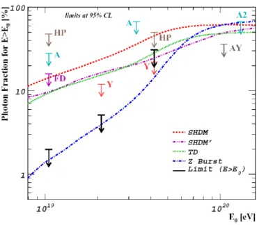
A distinctive feature of all top-down models and the Z-burst model is the prediction of a large photon flux at high energies. Therefore, the photon fraction of the total UHECR flux is a crucial test for these non-acceleration models [24, 25, 26].

The Pierre Auger Collaboration has set an upper limit on the photon fraction above 10 EeV which is twice as strong as those given previously [27]. This photon limit is obtained from the direct observation of the discriminat-ing observable, the depth of shower maximum Xmax, usdiscriminat-ing the fluorescence technique. Although the method supposes a great advantage since it not rely

Figure 1.10: Upper limits at a confidence level of 95% to the cosmic ray photon fraction derived in (Auger) and those previously obtained from AGASA (A1, A2) and Haverah Park (HP) data, compared to expectations for non-acceleration models (TD: topological defects, SHDM: superheavy relic particles, ZB: Z-burst model) [28].

on the simulation of nuclear primaries (subject to large uncertainties from modelling hadronic interactions), the derived upper limit to the photon frac-tion of 16% is limited by a low statistics and it is not able to test the photon flux predicted by top-down models. A more recent and stringent limit on the photon flux, obtained using the large statistics accumulated with the array of surface detectors at the Pierre Auger Observatory, is presented in [28] to-gether with an improvement of previous measurement, using the fluorescence detector. Now the maximum flux of photons has been constrained above dif-ferent energy limits to 2.0%, 5.1% and 31% at 10, 20 and 40 EeV respectively (see Figure 1.10).

These results are discussed in [29] showing that the models based on the decay of superheavy dark matter in the halo of our Galaxy are essentially excluded from being the sources of UHECR unless their contribution becomes significant only above around 100 EeV. For models based on topological defects the results are not so conclusive since some of them are compatible with the current limits and may be best constrained by the high-energy neutrino flux limit [30].

E_lab (eV) < X max > (g cm -2 ) proton iron photon photon with preshower QGSJET 01 QGSJET II SIBYLL 2.1 Fly´s Eye HiRes-MIA HiRes 2004 Yakutsk 2001 Yakutsk 2005 CASA-BLANCA HEGRA-AIROBICC SPASE-VULCAN DICE TUNKA 400 500 600 700 800 900 1000 1100 1200 1014 1015 1016 1017 1018 1019 1020 1021

Figure 1.11: Xmax as a function of energy measured by different experiments compared with predictions of different hadronic models for proton and iron showers.

1.2.5

Composition

For cosmic rays of low energies (up to about 1015_{eV) the particle flux is high}

enough to allow a direct detection which also provides valuable information about their composition. For this energy range the composition of cosmic rays have been found to be rather similar to those in the interstellar medium with some small differences that have been explained using the spallation of heavy nuclei to lighter ones.

Above these energies direct identification of the primary particle is not possible and cosmic rays are studied through the air showers that they de-velop in the atmosphere. One of the methods used to estimate the primary mass is based on the measurement of Xmax , defined as the atmospheric depth where the longitudinal development rises the maximum number of par-ticles. The elongation rate theorem proposed by Linsley in 1977 [31] shows that the average value of Xmax at a certain energy is related to the mass of the primary particle. Figure 1.11 shows the maximum depth Xmax as a function of energy by from different experiments. As it can be observed,

for energies up few times 1016 _{eV the composition is mainly dominated by}

iron nuclei. This fact is probably related with the limit of the efficiency of SNRs to accelerate cosmic rays since their radius becomes comparable to the Larmor radius of the particles. As the maximum energy attainable in

SNRs is proportional to the particle charge, iron nuclei will be accelerated

to higher energies than lighter primaries. Above more or less 6 × 1016 _eV

the experiments with data in this region, HiRes-MIA [32], HiRes [33], Fly’s Eye [34] and Yakutsk [35], suggest a change in the composition from a heavy

blend to a flux mainly dominated by proton primaries close to 1019 _{eV. The}

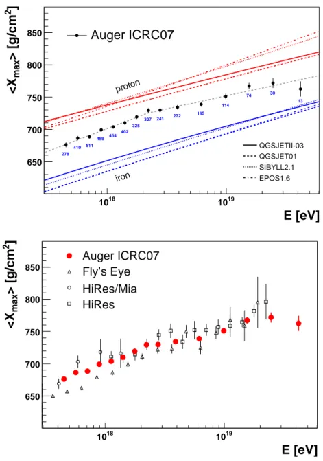
Pierre Auger Collaboration has estimated the variation of Xmax for the re-gion of UHECR [36] and the results are shown in Figure 1.12. Data are well described by a double linear fit (dashed gray line in the left panel of

Fig-ure 1.12) allowing for a break in 2.2 × 1018 _{eV. The slope of the fit is the}

so-called elongation rate. Though measurements favour a mixed composition for all energies, detailed interpretations are ambiguous since they are sub-ject to the uncertainties in the hadronic interactions at the highest energies. Whereas some models suggest a moderate lightening of the primary mass at low energies and a constant composition at high energies, other ones suggest a transition from light to heavy elements at high energies.

1.3

Extensive air showers and cosmic ray

de-tection

It is not possible to use satellite or balloon based detectors to study ultra high energy cosmic rays, due to their small flux: they have to be detected through the extensive air showers they produce in the atmosphere. When a cosmic ray primary undergoes an inelastic collision with an atmospheric nucleus its energy is shared between the products of the collision. Then, the created particles suffer successive collisions, giving rise to successive generations of shower particles.

Extensive air showers can be electromagnetic or hadronic, depending on the nature of the primary particle. In an hadronic shower induced by a baryon more than 90% of the energy is channeled into electromagnetic subshowers,

via the decay of the π0 _{produced in the hadronic interactions.}

Electromagnetic showers, induced by photons or electrons, are governed by two processes: photons undergo pair production while electrons/positrons radiate bremsstrahlung photons. The size of the shower grows until the mean energy of the electrons falls below the critical energy and ionization losses overcome bremsstrahlung. The hadronic showers are characterized by the interactions of the primary hadron in the atmosphere, that will generally a number of charged and neutral pions. Neutral pions decay into two photons so the energy they carry is channeled into two electromagnetic subshowers.

E [eV] 18 10 1019 ] 2 > [g/cm max <X 650 700 750 800 850 _{Auger ICRC07} 278 410 511 489 454 402 325 307 241 272 185 114 74 30 13 QGSJETII-03 QGSJET01 SIBYLL2.1 EPOS1.6 proton iron E [eV] 18 10 1019 ] 2 > [g/cm max <X 650 700 750 800 850 Auger ICRC07 Fly’s Eye HiRes/Mia HiRes

Figure 1.12: Xmax as a function of energy measured by the Pierre Auger Observatory. Data are compared to predictions from different hadronic interaction models for proton and iron primaries (up), and to data from previous experiments (down). [36].

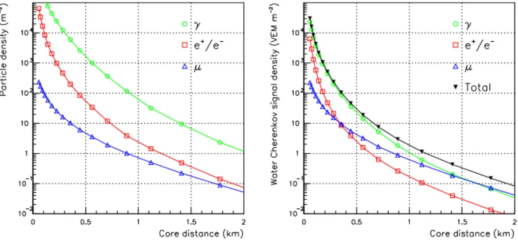
Figure 1.13: Left plot: lateral distribution at ground level of a simulated 1019

proton shower. Right plot: expected signal in a water ˇCerenkov detector [40].

having high factor, they will suffer a new interaction, without decaying. This will result in a new generation of charged and neutral pions and with them another fraction of the primary energy transferred into electromagnetic sub-showers. Eventually some of the created charged pions will decay to a muon neutrino pair: this constitutes the fraction of the primary energy that, differ-ent to the electromagnetic compondiffer-ent, will not be ultimately deposited in the atmosphere. Its value depends slightly on primary energy and composition but is around 10% of the firsts.

The study of air shower processes is necessary to extract the relevant information, most notable primary energy and mass, from shower measure-ments. A detailed description of cosmic ray shower phenomenology is out of the scope of this thesis. We will limit to a very brief introduction of the main experimental techniques, complemented with the relevant aspects of extensive air showers. Excellent reviews of air shower phenomenology and ultra high energy cosmic ray experimental techniques are found in the liter-ature [13][37][38][39][40].

Surface detectors

Surface detectors sample the extensive air shower at ground by means of an array of particle detectors. The shower is essentially a disc of particles moving at speed of light. When it strikes the ground, the particles are spread away from the shower axis (defined by the direction of the primary) due to the combined effect of multiple Coulomb scattering and traverse momentum in

0 1 2 3 4 5 6 7 200 400 600 800 1000 1200 1400 1600 1800 DPMJET 2.55 QGSJET 01c QGSJET II SIBYLL 2.1 atmospheric depth (g/cm2)

number of charged particles

× 10 9 Fe p γ E₀ = 1019eV vertical γ -induced

Figure 1.14: Simulated longitudinal profiles for proton, iron and photon primaries with an initial energy of 1019

eV and arriving at a zenith angle = 0◦ _.

shower interactions. The particle distribution is symmetric around the axis and its density falls with the distance to the core (Figure 1.13). Although the density distribution is characterized by the Moli`ere radius [41], about 100 meters at ground level [40], in the higher energy events it is possible to detect particles some kilometers away from the core. Surface detectors measure essentially the lateral distribution of the density of particles in the shower.

The energy of the primary is determined in surface detectors (in an in-direct manner) from the measured lateral distribution. Essentially, a Monte Carlo program is used to simulate high energy showers in the atmosphere, predicting the relation between energy and particle density. At the ground, one of the main indicators of the primary mass is the shower muon content. Thus, surface arrays use muon separation capabilities, both direct (placing underground muon counters) or indirect (separating the detector signal due to muons) to achieve mass composition sensivity. Its also possible to study the primary mass using the timing of the shower front: since muons suffer less scattering they tend to arrive earlier than the electromagnetic compo-nent [42].

Surface detectors use generally scintillators or water ˇCerenkov tanks as

compared to thin scintillators which are usually more difficult to build and deploy. Both methods are robust and reliable, well known, detectors adequate to instrument the required large areas.

Fluorescence detectors

Fluorescence detectors record the near UV light emitted by deexcitation of

N2 molecules previously excited by the shower particles. They provide a

di-rect measurement of the longitudinal shower development (Figure 1.14). This is crucial, because the integral of the profile is a direct measurement of the energy deposited in the atmosphere. Moreover, the depth of the shower max-imum is also a good indicator of the primary mass. Three factors limit the ability to study cosmic ray primary composition: intrinsic fluctuations on shower development, finite detector resolution and systematics and limited knowledge of high energy hadronic interactions.

Chapter 2

The Pierre Auger Observatory

The Pierre Auger Observatory [43], operated by an international collabora-tion, is conceived with the aim of measuring the spectrum, arrival direction and composition of UHECR with unprecedented statistics and with low sys-tematic uncertainties.

The Southern Observatory, completed in May 2008, is located near the

town of Malarg¨ue in Argentina. at the latitude of 35◦ _{South. The northern}

site is in its planning stage, in southeastern Colorado near the city of Lamar,

at an altitude of 1100 m above sea level (a.s.l.) and at the latitude of 38◦

North. Both Observatory provides a full sky coverage when combined. The need of full sky coverage is motivated by anisotropy studies, point source determination and correlations with astrophysical objects, as well as for determining the cosmic ray flux in different regions of the sky, since a different energy spectrum could give insides into different mechanisms of particle acceleration at the source.

The design incorporates two measurement techniques used with success in the past: detecting the Nitrogen fluorescence in the atmosphere caused by particles of the extensive air shower and measuring the lateral distributions

of particles that reach the ground. It consists of an array of water ˇCerenkov

detectors covering 3000 km2 _{with about 1600 detectors spaced 1.5 km apart}

in a triangular grid. The mean ground slope of less than 1% and the altitude of 1400 m ensures a measurement of the air shower at the same shower age, close to the maximum of the shower development of cosmic rays in the EeV range. On the edges of the Surface Detector array there are 4 fluorescence detector sites, each with 6 telescopes. The layout of the Southern Observatory is shown in Fig. 2.1.

The large surface detection area allows the collection of a large amount of statistics for analysis in a reasonable amount of time. With both detector sites completed and operational, the cosmic ray flux will be measured within

50 days with more statistics than the total of all experiments in the last 30 years. The stereo observation mode, by two or more fluorescence detectors, allows the understanding and the evaluation of the systematic effects arising from varying atmospheric conditions.

Most importantly the golden hybrid events, air showers recorded and reconstructed with both techniques, are useful for inter-calibration and data consistency checks.

Figure 2.1: The Pierre Auger Observatory, the red point are the ˇCerenkov counters, the 4 sites for the fluorescence telescope are indicated by names.

2.1

Surface Detector

The Surface Detector measures the front of the shower as it reaches ground. The tanks activated by the event record the particle density and the time of arrival. A wireless local area network (LAN) is used to communicate the tanks with four antennas at each fluorescence site. From there, the data is routed through a high capacity microwave link to the central data acquisition system (CDAS). Synchronization is provided by the standard GPS system.

2.1.1

Surface Detector unit

The cell unit of the Surface Detector (SD) of the Pierre Auger Observatory is a water Cherenkov counter. Each counter is a polyethylene tank of

cylin-drical shape with size 10 m2 _{x 1.2 m filled with purified water. Cherenkov}

light produced by charged particles of the showers is detected by three 9” photomultipliers. Each unit is autonomous with a battery and a solar panel (Fig. 2.2). Tanks are calibrated using the signals of atmospheric muons, a

Figure 2.2: A picture (up) and a schematic view (down) of a Surface Detector unit.

Figure 2.3: Topology of the concentric rings or hexagons used for T3 trigger decision [44].

proportional to the geometric path length. A test tank was used to estab-lish the relation between the signal of down-going vertical and central muons (VEM) and the peak of the histogram obtained from omni directional muons crossing the tank. Each station is calibrated matching the photomultipliers gain to obtain the expected trigger rate over a given VEM threshold. This procedure allows to calibrate the stations with respect to the absolute value of the VEM with an overall precision of 5%.

2.1.2

Data acquisition and triggers

Each station is equipped with three photomultipliers [45]. Two signals are extracted from each tank PMT Photonis XP1802: the signal from the last dynode and that from the anode. The last dynode signal is amplified to match the dynamic range. The anode is used for high signals such as seen when the station is near the core of the shower. The six signals from each tank are digitized by 10 bit fast analog to digital converters (FADCs) running at 40 MHz.

There are two types of local station triggers (T1): single threshold, a 3-fold coincidence of signals above 1.75 VEM and time over threshold, a 2-3-fold coincidence of 12 bins above 0.2 VEM within a 120 bins (a 3 µs window). T1 trigger rate is around 110 Hz. Upon a trigger, 256 pre-trigger and 512 post-trigger bins are stored in local buffer waiting for further post-trigger decisions to be taken.

Figure 2.4: Illustration of a minimum “2C1&3C2&4C4” condition. Triggered tanks are represented as full points. The first ring has one trigger (2C1 condition). The triggered tank in the second ring fulfills the 3C2 condition. The last tank can be as far as in the fourth ring because of the 4C4 condition.

The second level trigger (T2) is a software station trigger. All time over threshold triggers, and all threshold triggers above 3.2 VEM, are designated as T2. The local station controller, a CPU board running under the OS9 operating system, provides the T2 trigger decision as well as the handling of the GPS timing board, of the slow control board and of the forwarding of T2 triggers to CDAS. The rate of T2 triggers is around 20 Hz.

Whenever a station fulfills one of the T2 trigger condition, the trigger timestamp and the type of trigger are forwarded to CDAS. Within CDAS the central trigger receives the T2 and is used to identify groups of stations that are clustered in time and space to form a T3 trigger. Placing a 25 µs window at a given T2, the stations that have a trigger within this window are examined for spatial correlation. At least three T2 triggered stations are required (4-fold condition). At least one of the three has to be in one of the six adjacent stations that are closer to the triggered tank used as the time window center (the first ring, figure 2.3). Two of the three have to be within the second ring. The third has be within the fourth ring. This is known as the “2C1&3C2&4C4,” mCn meaning m triggered stations within the nth ring (see figure 2.4). In case of time over threshold (ToT) triggers, 3-fold coincidences fulfilling a “2C1&3C2” condition are also considered for a trigger. Once the spatial coincidence is verified, a final timing criteria is

imposed: each T2 must be within (6 + 5n) µs of the central one, where n represents the hexagon number. If this latter condition is fulfilled, the event is considered a T3 and CDAS requests the FADC data from the triggered stations.

The total trigger rate depends on the array size and CDAS can adequately handle rates at the level of 0.01 Hz. As the array is growing, the T3 trigger conditions are being strengthened to keep acceptable trigger rates.

The lowest CDAS trigger (T3) identifies time coincidences between the signals in different tanks that could be associated with a real air shower. It does not guarantee that the data are physics events while a large number of chance coincidences in accidental tanks is expected due to low energy showers and to single cosmic muons. It considers any of the following requests:

• a 3-fold condition, which requires a coincidence within a time interval depending on the distance of three tanks passing the ToT condition. • a 4-fold coincidence which requires the coincidence within a time

win-dow depending on the tank distance among 4 tanks having passed any T2 condition, with 2 tanks inside 2 hexagonal crowns from a triggered tank and a further one within 4 crowns. A crown is formed by the sta-tions at equal distance from the center one and are numbered depending on this separation.

• a 3-fold condition which requires the coincidence of three aligned tanks passing any T2 condition.

• an external condition generated by the fluorescence detector (FD). Every time a station has a T2 trigger it sends a signal to the CDAS containing the trigger time. The station trigger times are sorted. One by one all stations within a sliding time window of 50 µs are searched for the above patterns. If a pattern is found, the search stops and a first event trigger is formed.

For every event, a readout of the entire array is done. Some other in-formation, e.g. the station position, id, calibration histograms and an error code, are also stored in the data file.

The T3 trigger does not ensure that the events that are taken are physi-cal events, but the philosophy is that a large set of events is recorded among which all the physical events are contained and the sorting is left for a sub-sequent analysis.

The first physics trigger (T4) was designed to distinguish air showers from random coincidences of single atmospheric muons and is also the first step to select reconstructible vertical events. It consists of:

• 3ToT trigger requires at least 3 stations with a ToT trigger in a non-aligned configuration. This simple compact trigger is not effective for events with large zenith angles due to the dominance in this case of the muonic component which gives origin to fast less spread signals. This requirement selects 99% of the events with zenith angle less than 60 (Fig. 2.5).

• 4C1 trigger is passed only by events that have 4 tanks with a T2 trigger each, and a configuration of one station with 3 close neighbors (Fig. 2.6).

Figure 2.5: Two possible 3TOT compact configurations.

Figure 2.6: The three (minimal) 4C1 configurations.

In all cases of the T4 trigger, compatibility in time between stations part of the trigger is required. The difference in their start time has to be lower than the distance between them divided by the speed of light, allowing for a marginal limit of 200 ns.

The quality trigger (T5) is meant to exclude events that fall too close to the edge of the SD array. For this class of events, due to a possible missing

Figure 2.7: The T5 configuration. The central station (blue) with the largest signal is surrounded by 6 functioning stations.

signal, the reconstruction of the air shower variables may not be reliable. Another reason is that it is very hard to compute the acceptance which would take into account events that are highly energetic but far away from the array. In such cases the trigger probability for 4 tanks on the edge of the array depends on fluctuations which are very hard to simulate.

This quality trigger is based on a criterion related to the core position: for the station with the largest signal it is required to have six nearest neigh-bors that were present and functioning (but not necessarily triggered) at the time of the shower impact (Fig. 2.7). This assures a good and unbiased reconstruction of the event.

2.2

Fluorescence Detector

The fluorescence detector (FD) consists of 24 telescopes located at four site, which are built on small elevations on the perimeter of the array (Fig. 2.1). The telescopes measure the shower development in the atmosphere by col-lecting the fluorescence light emitted by the atmospheric nitrogen molecules excited by the charged particles of the shower.

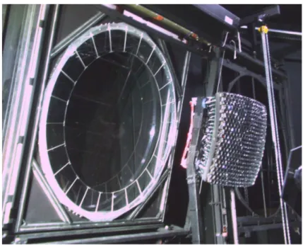
Each telescope is composed by an aperture system, a spherical mirror, and a 440 photomultiplier camera in the focal plane. A schematic view of the arrangement can be seen in figure 2.8. From left to right: shutters, aperture system with holding mounts for filter and corrector ring; camera with its support, mirror with support structure and, on the floor, the electronics crate.

Figure 2.8: A schematic view of the fluorescence telescope.

2.2.1

Optics

Each fluorescence telescope cover 28.6◦_{in elevation (from 2}◦ _{to 30.6}◦_{) and 30}◦

in azimuth. To achieve this large field of view with good optical quality the general layout of a Schmidt telescope has been adapted [46]: a diaphragm is used to limit the dimension of the aperture. The choice of Schmidt optics gives the advantage of eliminating coma aberration: the circle of least confusion, spot, caused by spherical aberration, is practically independent of the incident direction. The main disadvantage is that the focal surface of such a system is spherical, slightly complicating the camera design.

The diameter of the diaphragm is 1.7 m, giving an effective area for light

collection of 1.5 m2_{, after taking account of the shadow of the camera. The}

radius of curvature of the mirror is 3.4 m, and the angular size of the spot from spherical aberration is 0.5◦_{, i.e.} 1

Figure 2.9: Picture of a corrector ring, placed on its position in the aperture system.

As an extension of the Schmidt optics, a corrector ring is used to increase the light collection at the diaphragm maintaining the spot size [47]. Currently all the telescopes are equipped with corrector rings.

Aperture

The aperture system holds the diaphragm for the Schmidt optics design, the corrector ring, and an UV transmitting filter. The idea of an optical filter is to transmit most of the fluorescence signal in the near-UV while blocking other night sky background to which the PMTs are sensitive. The filter acts also as the window of the bay, protecting the telescope from the external environment [48]. Sheets of M-UG6 glass, 3.25 mm thick, are used. The filter efficiently transmits the nitrogen fluorescence spectrum in the near-UV, while blocking almost all visible light, which would increase the background noise.

A simple, but robust, support structure holds the glass sheets of 80 × 40 cm2

in place. The transmission curve peaks at about 85% for the wavelength of 350 nm and drops down to nearly 20% at 300 nm and 400 nm.

The background reduction due to the filter is a factor of 8. Since the fluctuations of the noise vary with the square root of the background, the expected signal to noise ratio improvement is factor of 2 [49].

the annular corrector ring [50], that increases the aperture to 2.2 m diameter. The corrector ring, of annular shape, has radial extension of 25 cm (inner radius of 0.85 m, as the original aperture, and outer radius of 1.10 m, fig-ure 2.9). It is constructed from 24 sectors made of UV transmitting glass, machined with an appropriate spherical profile to compensate for the spheri-cal aberration. The corrector ring nearly doubles the reference aperture area while maintaining essentially the same spot size.

Mirrors

The mirrors are of square form, 3.8 m×3.8 m in size, and are built up from smaller pieces held by a single common structure. The mirror pieces are attached to the supporting structure by means of an adjustable mount that allows the optimization of the orientation of the mirror segment to obtain a good overall alignment of the whole mirror.

There are two types of mirror segments: square aluminum mirrors and hexagonal glass mirrors [49]. They all share common performance require-ments, in particular 90% reflectivity between 300 and 400 nm and have a radius of curvature of 3.4 m.

Single mirrors are built upon 36 mirror segments (figure 2.10) aligned with respect to a removable reference point, placed on a strong and precise mechanical support, corresponding to the center of curvature of the mirror.

2.2.2

The camera

Because of the symmetry of the optical system, the actual focal surface is spherical in shape. It is concentric with the mirror and has a radius of 1.743 m,

slightly larger than the standard focal length. The camera segments the 30◦

azimuth × 28.6◦ _{elevation field of view into an array of 440 hexagonal pixels,}

with a 1.5◦ _{field of view each [51] (Fig. 2.11).}

Each pixel is defined by the light collectors, that improve the camera uni-formity and match the variable-size pixels to standard hexagonal photomul-tiplier tubes, the active light collecting devices. The pixel angular coverage is designed to optimize the signal-to-noise ratio and the sampling resolution of the shower profile.

Each pixel vertex is placed with equal angular separation over the focal surface. Equal steps in angle produce different linear dimensions depending on the pixel position on the spherical surface. Thus, pixels are not regular hexagons and their shape and size vary over the focal surface (figure 2.12). However, differences of the side length are smaller than 1 mm and are taken into account in the design of the light collectors [51].

Figure 2.10: Picture of an aluminum mirror, where each one of the single segments can be seen.

The camera body

Form the mechanical point of view, the main difficulty in camera design is to adapt its shape to the spherical focal surface.

The camera body is made of a single aluminum block. It consists of an ac-curately machined plate, 6 cm thick, approximately square (94 cm horizontal × 86 cm vertical) with inner and outer surface of spherical shape. The pho-tomultiplier tubes are positioned inside cylindrical holes which are drilled through the plate. Smaller drills serve as insertion points for the Winston cone holders.

The camera is held by a simple two-leg steel support, that results in an

ob-scuration area less than 0.1 m2 _{(about one tenth of the camera itself). Power}

and signal cables run inside the two legs of the support without producing additional obscuration.

Once in place, the camera is aligned with respect to the same reference point as the mirrors, by means of several mechanical adjustments provided in the base of the support and in the camera body fixing system. A ±2 mm alignment precision is achieved.

Figure 2.11: a) Detail of the camera body with four PMTs mounted together with two mercedes stars. The large holes to insert the PMTs and the small ones to mount the mercedes are clearly visible. b) Picture of a camera completely assembled with all PMTs and light collectors in place.

The photomultipliers and the Winston cones

Each pixel is instrumented with an eight-stage photomultiplier (PMT) tube, Photonis XP3062 (Fig. 2.14) , of 40 mm side-to-side hexagonal photocathode, complemented with light collectors. The photomultiplier array is made of 22 rows and 20 columns (figure 2.13). The hexagonal shape of the PMT cathode ensures optimal coverage of the focal surface.

The main characteristics of the PMT tubes are [52]:

Uniformity of response over the photocathode The response is uniform,

with a maximum ±15% of non-uniformity.

Spectral response The PMTs have a 0.25 average quantum efficiency in

the range 330-400 nm.

Figure 2.12: The linear dimensions of the pixels vary across the camera, because of the spherical geometry. Due to the details of camera construction there is also a small overlap region in the upper field of view of two neighbor telescopes, given by the pixels placed outside the 30◦ _{lines in the sketch.}

Linear dynamic range The PMT response is linear to better than 3%,

over a dynamic range of at least 104 _{for 1 µs signals. The maximum}

signal for linear response is expected to be 1 mA, corresponding to

6 × 104 _{photoelectrons for a gain of 10}5_.

Integrated anode charge The total anode charge is not less than 350 C, to

ensure the lifetime of the tubes, that will be operated under important levels of background light.

The PMTs are equipped with an active divider chain [53] and a preamplifier. The normal dark sky background induces an anode current at the level of 0.8 µA. The active divider ensures that the gain shift due to the divider chain is less than 1% for anode currents up to about 10 µA. Each PMT+base system is tested on a dedicated system, in addition to the test performed in the factory [54].

Figure 2.13: The photomultiplier camera and the Winston cones.

The base of the PMTs is soldered an includes two printed boards with the divider chain and the preamplifier [55]. A single cable carries the high voltage, the low voltage and the signal. The other end of the cable is attached to a distribution board at the back of the camera [56]. The distribution board serves 44 photomultipliers. Signals are driven through twisted-pair cable to the front-end board. A single power supply serves all the distribution boards of the whole FD site [57].

In order to maximize light collection and guarantee a sharp transition between adjacent pixels, each photomultiplier is surrounded by a simplified version of the classical Winston cones [58]. The designed light collectors [59] provide (1) a good matching of the hexagonal pixel geometry, (2) a sharp transition between adjacent pixels and (3) an almost complete recovery of the light falling on the insensitive area due to the space needed for safe mechanical packaging on the focal surface and the effective cathode area, that is smaller than the area delimited by the PMT glass envelope.

The cone is realized by a hexagonal set of flat reflecting surfaces. The basic element of the light collector is a mercedes star fixed at the vertex of three adjacent pixels (figure 2.15). The arm length is approximately half of the pixel side length while the arm section is an isosceles triangle. The base length of 9.2 mm is designed to match the photocathode inefficiency, 2 mm for each adjacent PMT, plus the maximum space between PMTs glass sides,

Figure 2.14: Picture of a PMT unit.

Figure 2.15: Each light collector unit has the form of a three point star. Six collector units correspond to an hexagonal pixel.

of the order of 5 mm. The triangle height is 18 mm, optimized taking into account the optical characteristics of the FD telescope, particularly the fact

that the light ray angles of incidence are between 10◦_{and 30}◦_{, approximately.}

The reflective surface is obtained by gluing aluminized Mylar on the mercedes surface.

The properties of the light collectors were tested [59] using a light source filtered in the 300-400 nm region which produced an image that simulated the spot created by the mirror, by means of a light diffusing cylinder. A small version of the full size camera body held seven Photonis hexagonal phototubes XP3062, arranged in a sunflower configuration. The light source was moved over the sunflower surface in steps of a few millimeters.

The recuperation of the light using the light collectors is demonstrated in figure 2.16, where the results of scanning a row of three adjacent pixels is

ε

Figure 2.16: Measurement of the light collection efficiency, ǫ, with a light spot moved along a line passing over three pixels. The full dots represent the measurements performed with the mercedes, while the open dots represent the measurements without the mercedes. In limited regions of the photocathode the light collection efficiency can be greater than one since is normalized to the average light collection efficiency integrated over the photocath-ode surface.

shown. At the photomultiplier edges the efficiency rises from about 50% to more than 90%. The light collectors are efficiently recovering the light loss. The uniformity within a given pixel is also improved, since light rays which were hitting the photocathode edges are now reflected on the mercedes and directed into the central region of the photocathode.

From these measurements, the light collection efficiency, ǫ, averaged over the FD focal surface was found to be 93% [59].

2.2.3

Electronics, trigger and DAQ

The fluorescence detector (FD) trigger is a 4 level trigger:

• The pixel trigger is built by four Field-Programmable Gate Arrays (FPGAs), each controlling 6 channels. The FADC values are integrated

over 10 bins improving the signal to noise ratio by a factor of√10. The

threshold is adjusted continuously to achieve a pixel trigger rate of 100 Hz.

• The second level trigger is also decided by the FPGA trigger board. It consists of a purely geometric pattern recognition. It searches for 4 or 5 adjacent pixels overlapping in a time window of 1 to 32 µs. The rate is 0.1 Hz per mirror.

• The last trigger is implemented in software. It checks for the time struc-ture of an event. The average trigger rate is 0.02 Hz per mirror. • After the last mirror-level trigger the data are collected by the eye PC,

where the events have to pass the eye trigger level T3 which performs rudimentary event reconstruction of the direction and of the time of im-pact on the ground that is used in CDAS for reading the corresponding part of the array.

The main tasks of the telescope electronics are to shape the PMT signals from FD cameras, to digitize, to store them, to generate a trigger based on the camera image and to initiate the readout of the stored data. A computer network compresses the data, refines the trigger decision, gathers data of the same event from different telescopes and transfers them to the central computing facility, CDAS [60].

The design of the system is aimed to obtain high reliability and robustness for 20 years of operation, good absolute time synchronization with the surface array stations, and flexibility in the trigger scheme.

The organization of the front-end electronics (FE) follows the structure of the telescopes in the FD buildings. Each of the 24 telescopes is readout by one FE sub-rack through its associated Mirror PC. Each sub-rack covers 22×20 pixels of the camera and contains 20 Analog Boards (AB), 20 First Level Trigger (FLT) boards and a single Second Level Trigger (SLT) board [61].

Analog electronics The analog signal processing starts at the Head

Elec-tronics (HE) which consists of 2 circular printed circuit boards (PCB) mounted directly behind the XP3062 hexagonal PMTs. The inner board holds an ac-tive voltage divider which allows the biasing of the PMT dynodes with low power dissipation and high linearity compared to a conventional design [62]. The outer PCB contains a differential-input and a balanced output driver to transfer the PMT signals with low noise and high dynamic range via twisted pair lines to the Analog Boards (AB) at the front-end sub-rack. The driver is located on a small hybrid circuit, which has a symmetrical layout and laser trimmed resistor pairs matched to 0.25% to reduce the common mode noise. The signals from the camera are processed by 20 AB, i.e. each board serves the 22 channels of a single camera column. The AB holds a differential line receiver, a programmable gain amplifier (to balance the gain spread of the

pixels) and a fourth order anti-aliasing filter in front of the ADC. A 15-bit dynamic range is achieved by introducing an additional low gain channel, which processes the rare large pulses. An on-board test-pulser allows injection of signals with programmable width and amplitude in each channel in order to check the full system even when the camera is not connected [55].

The measured noise for a PMT gain of 5 × 104 _{was smaller than 0.5}

pho-toelectrons in a 100 ns, 20% of the expected background due to the diffuse

sky light. The cross-talk was smaller than 6 × 10−4 _{and the linearity better}

than 2% (4% with a large continuous background) [63].

Digital electronics, DAQ and trigger The PMT signals are digitized

using 10 MHz 12 bit Flash ADCs. The digital part of the front-end board is used to implement all functions of the First Level Trigger (FLT) with re-programmable logic chips. The trigger logic also implements the calculation of the pixel ADC variance, which is proportional to the DC background light. The knowledge of the background level allows to protect the PMTs against excess of natural or artificial light as well as providing an useful method to study the detector pointing through the record of start tracks [64].

The SLT logic is implemented on a separate board, which is used to read the pixel triggers generated for each channel in the 20 FLT boards. The SLT algorithm is used to search for patterns of five pixels consistent with a track segment, and to generate an internal trigger for data readout. Synchronization with the front-end board is provided by a GPS clock.

The Mirror PC, a robust, disk-less, industry PC associated with each telescope, is used to perform the data readout and the associated software triggers.

The timing synchronization precision is guaranteed using the GPS stan-dard and is monitored through the Central Laser Facility: the same laser signal can be detected by each Fluorescence Detector and fed to a single SD tank (Celeste). Such generated events are monitored in search of any timing shifts between detectors [65].

Slow Control The task of the FD Slow Control System (SCS) [66] is to

control and supervise the operation of each FD telescope. It relies on a series of sensors to monitor the environmental conditions (such as ambient light or wind velocity) and the status of different devices (such as PMTs HV system or shutters).

One of the slow control key aspects is the ability to implement security policies in the data taking context: automatic HV shutdown or shutter closing when ambient safety conditions (i.e. ambient light or wind force) are not

fulfilled.

2.2.4

Detector Calibration

Calibration is essential to convert measured ADCs into light fluxes, that can be then translated to energy deposition. The absolute calibration of the fluo-rescence detectors uses a calibrated 2.5 m diameter light source, the drum, at the telescope aperture, providing uniform illumination to each pixel. Unifor-mity of light emission from the drum surface is important, since the pixels in an Auger fluorescence detector camera view the aperture at varying angles.

The detector is calibrated end-to-end, including optical transmission of the aperture and the mirrors, camera shadow, pixel area, light collection and photomultiplier quantum efficiency. The drum illuminator [67] is a pulsed

Figure 2.17: Left: photograph of the drum structure. The light source is placed on the mount inside, directed to the rear walls. All the inside walls are covered with Tyvek while a sheet of Teflon is placed on the front. Right: CCD picture of the drum light output. Different colors mean different light intensities. Except for the borders and the central light source shadow the output light intensity is rather uniform. The black concentric circles are drawn to guide the eye.

UV LED, emitting in a narrow band around 375 nm, embedded in a small cylinder of Teflon, illuminating the interior of a 2.5 m diameter cylindrical drum, 1.4 m deep. The sides and back surfaces of the drum are lined with Tyvek, while the front face is made of a thin sheet of Teflon, which transmits light diffusely (figure 2.17).

To calibrate each telescope, the drum is mounted on the the aperture. The provided illumination is uniform within 3%. The drum itself is calibrated using a NIST-calibrated photodiode, that measures the absolute light flux

to a precision of about 7%. The absolute calibration is derived from the telescope response under drum illumination [68].

A cross-check calibration can be obtained firing a nitrogen laser in the telescope field of view [69]. If the laser power is known, the amount of light reaching the telescope comes mainly from the well known Rayleigh scattering, provided that the laser is fired not far from the telescope. Since it depends on atmospheric conditions and requires placing the laser in each one of the tele-scopes field of view, this method is only used as a cross-check. This absolute calibration of the detector has currently an uncertainty of 12%.

Relative calibration An optical system for relative calibration is used to

monitor possible time variations in the calibration of the telescopes [70], that are subjected to absolute calibration only from time to time. Three Xenon flash lamp light sources per building, coupled to optical fibers, are used to distribute light signals into three locations at each telescope: the center of the mirror (with the light directed to the camera), the sides of the camera (with the light directed to the mirror through a Teflon diffuser) and the sides of the entrance aperture (with the light directed to a reflective Tyvek target mounted on the telescope doors, from which it is reflected back into the telescope). The optical system is completed with neutral density and interference filters (to monitor the stability at different wavelengths in the range of 330-410 nm).

2.2.5

Atmospheric Monitoring

A precise determination of the fluorescence light emitted by the cosmic ray shower must take into account the attenuation of the light in its passage from the emission point to the detector. A detailed knowledge of the scat-tering properties of the atmosphere and its time dependence is mandatory. A full program, composed of different, complementary approaches is being developed on site [71].

The principal component is the LIDAR, a steerable Laser system capable of measuring the atmospheric aerosol content by the backscattered light sig-nal [72]. The LIDAR is complemented by Horizontal Attenuation Monitors (HAM) that are able to measure the total extinction length between two fixed points and are a cross-check to the LIDAR. Cloud monitors use near infrared photography to check the cloud coverage over the telescopes [73]. The atmospheric monitoring program is completed with the periodic launch of balloon based radiosondes to study the molecular atmospheric profiles [74]. The data is taken every 20 m in altitude until reaching 25 km (a.s.l.). The