An information theory analysis of critical Boolean networks as control software for robots

(1)

DIPARTIMENTO DI INFORMATICA - SCIENZA E INGEGNERIA CORSO DI LAUREA MAGISTRALE IN INGEGNERIA E SCIENZE

INFORMATICHE

An information theory analysis of

critical Boolean networks as

control software for robots

TESI IN

SISTEMI INTELLIGENTI ROBOTICI

Relatore:

Prof. ANDREA ROLI

Co-relatore:

Dott. MICHELE BRACCINI

Presentata da:

Dott. MATTEO MAGNINI

Anno accademico

2019 - 2020

(2)

In arduis servare mentem

(Aircraft carrier Cavour)

(3)

(4)

Abstract

This work is an analysis of critical random Boolean networks used as control software for robots. The main goal is to find if there are relations between information theory measures on robot’s sensors and actuators and the capability of the robot to achieve a particular task. Secondary goals are to verify if just the number of nodes of the networks is significant to obtain better populations of controllers for a given task and if a Boolean network can perform well in more than one single task. Results show that for certain tasks there is a strongly positively correlation between some information theory measures and the objective function of the task. Moreover Boolean networks with an higher number of nodes tend to perform better. These results can be useful in the automatic design process of control software for robots. Finally some Boolean networks from a random generated population exhibit phenotypic plasticity, which is the ability to manifest more phenotypes from the same genotype in different environments. In this scenario it is the capability of the same Boolean network (same functions and connections) to successfully achieve different tasks.

(5)

(6)

4.2.1 Obstacle Avoidance . . . 24 4.2.2 Path Following . . . 26 4.2.3 Phototaxis . . . 27 5 Results 29 5.1 Obstacle Avoidance . . . 30 5.1.1 Objective function . . . 30 5.1.2 Measures . . . 33 5.1.3 Correlation . . . 34 5.2 Path Following . . . 44 5.2.1 Objective function . . . 44 5.2.2 Measures . . . 46 5.2.3 Correlation . . . 47 5.3 Phototaxis . . . 58 5.3.1 Objective function . . . 58 5.3.2 Measures . . . 60 5.3.3 Correlation . . . 61 5.4 Switched controllers . . . 72 5.4.1 Objective functions . . . 72 5.4.2 Sensor entropy . . . 74 5.4.3 Predictive information . . . 75 5.4.4 Transfer entropy . . . 76

5.4.5 Reverse transfer entropy . . . 77

Conclusion 79

(8)

List of Figures

1.1 entropy 1.1 curve shape in the case of an aleatory Boolean variable. . . . 2

1.2 diagram showing the properties for functions entropy (H) and mutual information (I). . . 4

2.1 on the left a graph representing a Boolean network, on the rights the nodes’ Boolean functions as truth tables. . . 8

2.2 shape of function 2.1 for critical Boolean networks. . . 11

2.3 high level architectural scheme of the robot’s controller. . . 12

3.1 real foot-bot view. . . 17

3.2 placement of sensors and actuators. . . 18

3.3 ARGoS GUI. . . 19

4.1 obstacle avoidance arena. . . 25

4.2 path following arena. . . 27

4.3 phototaxis arena. . . 28

5.1 Foa score distributions. . . 31

5.2 obstacle avoidance paths for top 20 robots with respect to Foa. . . 32

5.3 SE score distributions for obstacle avoidance. . . 33

5.4 Measures score distributions without SE for obstacle avoidance. . . 34

5.5 SE - Foa plot for networks with N = 20. . . 35

5.8 obstacle avoidance paths for top 20 robots with respect to SE. . . 37 v

(9)

5.9 PI - Foa plot for networks with N = 20. . . 38

5.12 obstacle avoidance paths for top 20 robots with respect to PI. . . 39

5.13 TE - Foa plot for networks with N = 20. . . 40

5.14 obstacle avoidance paths for top 20 robots with respect to TE. . . 40

5.17 RTE - Foa plot for networks with N = 20. . . 42

5.20 obstacle avoidance paths for top 20 robots with respect to RTE. . . 44

5.21 Fpf score distributions. . . 45

5.22 path following paths for top 20 robots with respect to Fpf. . . 46

5.23 Measures score distributions without SE for path following. . . 47

5.24 SE score distributions for path following. . . 48

5.25 SE - Fpf plot for networks with N = 20. . . 49

5.28 path following paths for top 20 robots with respect to SE. . . 50

5.29 PI - Fpf plot for networks with N = 20. . . 51

5.32 path following paths for top 20 robots with respect to PI. . . 53

5.33 path following paths for top 20 robots with respect to TE. . . 53

5.34 TE - Fpf plot for networks with N = 20. . . 54

5.37 RTE - Fpf plot for networks with N = 20. . . 56

5.38 RTE - Fpf plot for networks with N = 50. . . 56

(10)

vii

5.40 path following paths for top 20 robots with respect to RTE. . . 57

5.41 Fpt score distributions. . . 58

5.42 phototaxis paths for top 20 robots with respect to Fpt. . . 59

5.43 SE score distributions for phototaxis. . . 61

5.44 Measures score distributions without SE for phototaxis. . . 62

5.45 SE - Fpt plot for networks with N = 20. . . 63

5.48 phototaxis paths for top 20 robots with respect to SE. . . 64

5.49 PI - Fpt plot for networks with N = 20. . . 65

5.52 phototaxis paths for top 20 robots with respect to PI. . . 67

5.53 phototaxis paths for top 20 robots with respect to TE. . . 67

5.54 TE - Fpt plot for networks with N = 20. . . 68

5.57 RTE - Fpt plot for networks with N = 20. . . 70

(11)

(12)

List of Tables

5.1 Foa Wilcoxon’s test. . . 31 5.2 Pearson’s correlations between information theory measures and Foa. . . 34 5.3 Fpf Wilcoxon’s test. . . 44 5.4 Pearson’s correlations between information theory measures and Fpf. . . 48 5.5 Fpt Wilcoxon’s test. . . 60 5.6 Pearson’s correlations between information theory measures and Fpt. . . . 62 5.7 SRBNs obtained by the top 20 RBNs with respect to the objective functions. 73 5.8 SRBNs obtained by the top 20 RBNs with respect to sensor entropy. . . 74 5.9 SRBNs obtained by the top 20 RBNs with respect to predictive information. 75 5.10 SRBNs obtained by the top 20 RBNs with respect to transfer entropy. . . 76 5.11 SRBNs obtained by the top 20 RBNs with respect to reverse transfer

entropy. . . 77 5.12 summary of SRBNs repartition . . . 78

(13)

(14)

Introduction

This work belongs to the field of Robotics, in particular Intelligent Robotic Systems. A robot is a complete physical autonomous agent able to perform a task in a real world environment without the human intervention. The work concerns also Complex Systems Science by using particular types of Boolean networks as control software for robot. Ultimately this work regards information theory by using metrics to measure information properties over the robot controller.

The reason for this work is not only to expand the scientific knowledge on information theory and Boolean networks but also to give more expertise in the automatic design of control software for robots. Automatic design of controllers holds a crucial role in robotics and Boolean networks can be successfully used in the process as control software [23]. The main objective of this work is to investigate if some measures of information theory could be used as a not handcrafted merit factor for automatic design in specific tasks.

This thesis analyzes the results of robots controlled by critical random Boolean net-works in predefined tasks. Three common tasks in robotics are chosen: obstacle avoid-ance, path following and phototaxis. Several experiments are executed with different network configurations through a simulation software. Results are collected in textual files for analysis. The goal is to find if there are relations between information theory metrics over robot’s sensors and actuators and handwritten task objective function. An-other objective is to verify if there are differences in networks populations with respect to robot’s ability in achieving a task. Finally controllers are switched in the other two tasks they did not see. The goal is to test if the same critical random Boolean network is capable of performing well more than one task.

(15)

The thesis is structured as follow. Chapter 1 introduces information theory measures used in the analysis. Chapter 2 describes Boolean networks with focus on their possible topologies and on critical Boolean network. Chapter 3 illustrates the simulation software use for the experiments along with the robot and its characteristics. Chapter 4 defines the tasks, in particular the arena, duration and objective function. Finally in chapter 5 the results of the experiments are reported along with their analysis.

(16)

Chapter 1 Information Theory

This chapter is an overview of the main concepts of information theory. In particular in section 1.1 some information theory measures are formally described. These measures are used in the experiments (see chapter 4) to evaluate Boolean networks, results are reported in chapter 5. An estimation of the computational cost needed to compute the metrics introduced is provided in section 1.2.

1.1 Measures

Information theory is a pervasive science whose subject is information related phe-nomena and information itself. The field of information theory spread in 1948, when C. Shannon published a paper [25] where he defined a mathematical notion by which information could be quantified. Information theory has found applications in several fields like cryptography [1], data compression [13], neuroscience [6], bioinformatics [26], robotics [3] [10], etc. In the literature many information measures have been proposed. Here we introduce the measures that we use in the experiments analysis 5.

1.1.1 Entropy

Entropy (H) is the measure that quantifies the amount of information carried by a source. A source can be considered as an aleatory variable related to some sort of event.

(17)

An event that is certain has entropy zero. An event whose outcomes are all equally probable, the maximum of uncertainty, has the highest entropy.

The discrete entropy’s formula introduced by C. Shannon [25] is:

H(X) = −X

x

p(x) log₂p(x) (1.1)

where X is an aleatory variable, x is one of its finite possible value, p(x) is the probability of X to be equal to x, an abbreviation for p(X = x). The curve equation for a Boolean variable is plotted in figure 1.1.

Figure 1.1: entropy 1.1 curve shape in the case of an aleatory Boolean variable, for example a coin toss where head has probability p, with p ∈ [0, 1], and tail 1 − p.

The choice of the base of the logarithm is arbitrary. For now on we always consider the base two. The unit of measure using the base two logarithm is called bit(s). The lower bound of H is zero, while the upper bound is:

(18)

1.1 Measures 3

1.1.2 Mutual Information

Mutual Information (MI) quantifies the amount of information shared by two aleatory variables. When the variables are independent MI is zero, while when they are fully dependent MI is maximized.

The discrete mutual information’s formula [25] is: M I(X, Y ) =X

x,y

p(x, y) ∗ log₂ p(x, y)

p(x) ∗ p(y) (1.3)

where X and Y are two aleatory variables, x and y are possible values of the variables and p(x, y) is the joint probability of the two variables, an abbreviation for p(X = x, Y = y). The lower bound of MI is zero, while the upper bound is the minimum entropy of the two variables:

M ax(M I(X, Y )) = M in(H(X), H(Y )) (1.4)

Proof:

Mutual Information can be rewritten as

M I(X, Y ) = H(X) + H(Y ) − H(X, Y ) (1.5) so, by contradiction M I(X, Y ) > H(X) H(X) + H(Y ) − H(X, Y ) > H(X) H(Y ) > H(X, Y ) but H(Y ) <= H(X, Y ) ∀X, Y so M I(X, Y ) <= H(X) (1.6)

and for symmetry M I(X, Y ) <= H(Y ).

In figure 1.2 are summarized the main properties for functions H and MI (I in the figure) with different relations between the aleatory variables.

1.1.3 Predictive Information

“Observations on the past provide some hints about what will happen in the future, and this can be quantified using information theory’ ’[4]. W. Bialek and N. Tishby

(19)

Figure 1.2: diagram showing the properties for functions entropy (H) and mutual infor-mation (I). Red circle represents H(x), blue circle is H(y), green circle is H(z). Overlap-ping circles means partial dependency between the involved aleatory variables. Figure taken from [27].

introduced in 1999 a measure to quantify information sharing across time between two variables. We call predictive information (PI) the quantity of shared information between variable X and Y (time series) considering the latter at time t + c, c is a positive constant that we consider always 1 in the experiments. With c = 1 we fall into Markov processes which hypothesize that the past information contained in the previous step holds the entire information needed. The discrete predictive information’s formula is MI considering the second variable one step ahead in the future:

P I(X, Y ) = M I(Xt, Yt+1) = X yt+1,xt p(xt, yt+1) ∗ log2 p(xt, yt+1) p(xt) ∗ p(yt+1) (1.7)

This function can be easily applied in many ways for measuring the complexity of a system. In [3] PI is computed on a robot’s sensor values at time t and on sensor values at

(20)

1.1 Measures 5

time t+1. Researchers have found that for the particular task and environment that they were analysing PI is high when the robot has a explorative behaviour and predictable future sensor values. PI is proposed as a candidate objective function for similar scenario. Instead, in [10], PI is computed on sensor values at time t and on actuator values at time t + 1. PI is used, along with other measures of complexity, to evaluate robots during an evolution process in the achievement of a given task.

1.1.4 Transfer Entropy

Intuitively, transfer entropy (TE) is the amount of directed, time asymmetric, in-formation exchanged over time from an aleatory variable X towards another one Y . Introduced by T. Schreiber[24], the most general discrete formula is:

T EX−→Y = T E(X, Y ) = X yt+1,ytk,xlt p(yt+1, ytk, x l t) ∗ log2 p(yt+1|ykt, xlt) p(yt+1|ytk) (1.8)

where p(yt+1|ytk, xlt) is the conditional probability of yt+1 given ytk, xlt, similarly for the other conditional probability. The apexes k and l indicates the amount of delay to consider: yk

t is an abbreviation for (yt, ..., yt−k+1). For ease of computational power we always consider k = l = 1. Like for the choice of c = 1 in PI, choosing k = l = 1 is equivalent to consider the entire past and the entire future for Markov processes.

Transfer entropy can be rewritten in function of simpler measures:

T E(X, Y ) = H(Yt+1|Yt) − H(Yt+1|Yt, Xt) (1.9) It is straightforward to see that the lower bound is zero, while the upper bound is the minimum of the entropies of X and Y.

M ax(T E(X, Y )) = H(X) (1.10)

Proof:

H(Yt+1|Yt) = H(Yt+1, Yt) − H(Yt)

H(Yt+1|Yt, Xt) = H(Yt+1, Yt, Xt) − H(Yt, Xt)

T E(X, Y ) = H(Yt+1, Yt) + H(Yt, Xt) − H(Yt) − H(Yt+1, Yt, Xt) M I(Yy+1, Xt|Yt) = H(Yt+1, Yt) + H(Yt, Xt) − H(Yt) − H(Yt+1, Yt, Xt) 0 <= M I(Yy+1, Xt|Yt) <= M in(H(Xt), H(Yt+1))

(21)

so M ax(T E(X, Y )) = M in(H(X), H(Y )).

1.2 Computational cost

To calculate the previous measures one must known the required probabilities. It is worth to spend some words about the computational cost of this operation. Indeed, if we want to compute the exact value of a measure previously introduced this could result in a time expensive calculus.

Lets suppose to have a file with the values of two time series, named X and Y . A row contains the value of a time step for X and Y , L is the file length.

• H(X). We have to compute all the probabilities for each value of X then the summation in X. So the cost is L|X| + |X| = O(L|X|);

• MI(X, Y ) or P I(X, Y ). We have to compute all the probabilities for each value of X, Y and the joint probability. Then we have to compute the two summations in X and Y . Cost is L(|X| + |Y | + |X||Y |) + |X||Y | = O(L|X||Y |);

• T E(X, Y ). It can be rewritten as

T E(X, Y ) = X yt+1,yt,xt p(yt+1, yt, xt) ∗ log2 p(yt+1, yt, xt) ∗ p(yt) p(yt, xt) ∗ p(yt+1, yt) (1.12)

We have to compute all the probabilities for each value of Xt, Yt+1 and Yt, however the latter two have the same ones. Then the joint probabilities for < Yt, Xt >, < Yt+1, Yt >, and < Yt+1, Yt, Xt >. In the end the three summations in Xt, Yt and Yt+1. Cost is L(|X| + |Y | + |X||Y | + |Y |2+ |X||Y |2) + |X||Y |2 = O(L|X||Y |2). Cost for TE is linear in the file length and in the number of results of variable X. It is polynomial in the number of results of variable Y . This turns out to be the most expen-sive measure to compute. If the time cost is too expenexpen-sive or in the case of continuous aleatory variables, one can use approximation techniques to estimate the probability distributions like KDE [19].

(22)

Chapter 2 Boolean Networks

In this chapter we introduce the concept of Boolean networks and the more common models, section 2.1, with a focus on critical Boolean networks. In section 2.2 a description is presented of how Boolean networks are used in experiments (4) as control software for robots.

2.1 Definition

A Boolean network is a discrete time and discrete state dynamical system. It can be instantiated as a directed graph where nodes hold both a Boolean value, 0 or 1, and a Boolean function, an example is represented in figure 2.1. The state of the network is the ordered set of its nodes’ values. So, if the number of nodes is N , the number of all possible states of the Boolean network is 2N. Vertices between nodes are oriented. A vertex carries the Boolean value of the starting node towards the ending node. A node computes its Boolean function based on the values of the incoming vertices and updates its Boolean value. The update scheme used in this work is always synchronous and deterministic. A Boolean function can be represented as a truth table and the number of possible functions is based on the number of incoming vertices. If ki is the number of incoming vertices for node ni, then ni has a Boolean function in a set of 22

ki

functions. A random Boolean network (RBN) is a Boolean network where vertices and Boolean functions are chosen randomly.

(23)

Figure 2.1: on the left a graph representing a Boolean network, on the rights the nodes’ Boolean functions as truth tables. Image taken from [22].

A Boolean network could have attractors. An attractor is a subset of the state space towards which a dynamical system evolves over time. The attractor can be a fixed point, one state, or a cycle, more states. Once a Boolean network reaches an attractor, if its update scheme is deterministic, it cannot reach states that are not in the set of the attractor. Dynamical systems can be analyzed using attractors’ characteristics like length, basin of attractor, etc. The basin of attractor is the set of states from which the system reach the attractor for t −→ +∞. The state space is divided into basins based on the amount of attractors.

Different strategies of connecting nodes rise to different network topologies, so differ-ent features:

• random graphs, this is the first topology and it is used as a benchmark for the other ones. Random graphs are generated through a random process, for example adding vertices to the graphs by randomly selecting two different nodes with an uniform distribution. The node degree distribution is Poissonian or Gaussian. The topology used for the experiments is a critical random Boolean network, also known as N-K model, described in section 2.1.1;

(24)

2.1 Definition 9

• grid-like networks, this is a very high ordered topology. Each node is connected with a predefined number of neighbour, generally few units. Real examples are computers grids and low-voltage networks;

• scale-free networks, qualitative this topology has few nodes with many connections and the majority of nodes with few connections. More formally the node degree distribution follows a negative power low. These networks are robust to accidental damage, but vulnerable to specific attacks. They are also related to small world phenomena. This topology can represent several real systems such as social network relations, web pages, Internet, etc;

• small world networks, these networks have low mean path length between nodes and high clustering. They are in balance between random networks and grid networks. Scale-free topology Boolean networks have been proved to model well real systems such as genetic networks. Random Boolean networks, like the N-K model, can still reach discrete results but definitely they need to be fine-tuned[2]. Also Boolean networks with small-world topology have reached interesting results, they “have a propensity to combine comparably large information storage and transfer capacity”[16].

Besides the topology, Boolean networks can be distinguished by their updating scheme. Generally there are two main different updating scheme: synchronous and asyn-chronous. In the synchronous update scheme all nodes are updated at the same time. It is always deterministic, a Boolean network in state st updates towards the same state st+1. Instead, in the asynchronous update scheme nodes are updated one at a time. The single node update is still deterministic, however the whole network update can be random.

Updating schemes based on C. Gershenson’s taxonomy[11]:

• CRBNs, classic random Boolean networks were proposed by S. Kauffman[14] in 1969. The updating is synchronous and deterministic. CRBNs have attractors. Due to the determinism, once a CRBN reaches an attractor it can only have states belonging to the attractor (except for external perturbations);

(25)

CRBNs but the updating is asynchronous and random. At each time step a node is randomly selected and then updated, so they are not deterministic;

• DARBNs, deterministic asynchronous random Boolean network are like ARBNs but the choice of the node to update is not random. A node is selected following a rule based on a parameter that specify its update period. If more than one node have to update, then they are updated asynchronously following their order; • GARBNs, generalized asynchronous random Boolean networks are like ARBNs but

can update any number of node at each time step;

• DGARBNs, generalized asynchronous random Boolean networks are like DARBNs but if more than one node have to update, then they are updated synchronously.

2.1.1 Critical Boolean Networks

The number of incoming vertices for the node ni is expressed by parameter ki. If all nodes have the same value for ki, the network is homogeneous and it has a global parameter K equal to that value. The Boolean function for a node ni is a truth table with 2K rows where for each row the output is chosen randomly with probability pi to be set to 1. If all nodes have the same value for pi, the network has a global parameter p equal to that value.

Networks follow the N-K model introduced by S. Kauffman[15] when they have global parameter K, connections are randomly chosen with uniform probability and nodes have global probability p to be active (value 1). A system in a critical regime is said to be in between “order” and “chaos”[18]. If a Boolean network has a stable behaviour its dynamics are frozen, perturbations die out in short time. If it has chaotic behaviour attractors’ length is long, almost 2N_{, and it is heavily affected by small perturbations. A} Boolean network is critical when the attractors’ length is short, low degree polynomial of N . This kind of network is robust to small perturbations. Parameters K and p in critical Boolean networks follow the relation[9]:

Kc=

1 2 ∗ pc(1 − pc)

(26)

2.2 Boolean Networks as control software for robot 11

Figure 2.2: shape of function 2.1. Networks with parameters that are under the curve have frozen dynamics. Networks with parameters that are above the curve have long attractors. Networks whose parameters are on the curve are critical.

2.2 Boolean Networks as control software for robot

In the experiments we use critical RBNs without self loops as control software for robot. A moderate number of self loops makes RBNs more suitable to show differentia-tion phenomena[7]. Increasing the number of self loops raises the attractors but reduces robustness and stability[17]. The robot, detailed described in section 3.2, has a set of sensor Boolean values constantly updated over simulation time. The sensors are coupled with nodes of the network in a one-to-one relation. For each time step the nodes’ value of the coupled ones are forced to be equal to the corresponding sensor values, then the network is updated. A subset of nodes, with different nodes from the ones already used, are coupled with the robot’s actuators. The Boolean value of an actuator is forced to be a new value that is function of the corresponding node’s value. Figure 2.3 represents

(27)

the architectural scheme previously described.

Figure 2.3: high level architectural scheme of the robot’s controller. The robot acquires sensor information and forces sensor values into the network, blue nodes. Network up-dates its state and the Boolean values of the red nodes are used to set the actuator values. In the example of the image the Boolean network has N = 8 and K = 3.

We choose to use the following parameters for the networks: • N = 20, K = 3, p = 0.79;

• N = 50, K = 3, p = 0.79; • N = 100, K = 3, p = 0.79.

(28)

2.2 Boolean Networks as control software for robot 13

Self loops are not allowed and a node cannot output to the same node twice, furthermore nodes’ function and vertices do not change over experiment time, there is no network evolution.

The space of all the possible networks is more than exponential in K. We have to consider all the possible Boolean functions, the number of nodes and the possible ways of connecting nodes. The functions are 22K

so, with K = 3, they are 256. The number of ways of connecting nodes, because we do not allow self loops and allow only one directed connection from a node ni towards a node nj, is N − 1 for the first vertex, N − 2 for the second one and N − 3 for the third. The number of all possible networks is:

N etworks = 22K ∗ (N )K+1 (2.2)

With K = 3 the numbers of unique networks in function of the number of nodes are: • N = 20, networks = 29, 767, 680;

• N = 50, networks = 1, 414, 963, 200; • N = 100, networks = 24, 092, 006, 400.

Some of them are equivalent. By properly applying some operations on the network, like changing Boolean functions or connections, it is possible to obtain an equivalent one (same state transitions).

(29)

(30)

Chapter 3 ARGoS simulation software

This chapter describes the simulation software used for running the experiments. The simulation model and environments are presented in section 3.1. In section 3.2 the robot foot-bot is shown in detail along with its sensors and actuators. In the last section 3.3 is briefly described the GUI to inspect a single experiment.

3.1 Environment

The simulation software used for the experiments is ARGoS [20] (Autonomous Robots Go Swarming). ARGoS is a fast multi-robot simulator developed at IRIDIA, Artificial Intelligence research laboratory of the Universit´e Libre de Bruxelles. It is easy to use and versatile, it can handle different scenarios for several applications. ARGoS grants high accuracy, high flexibility and high efficiency. For accuracy it is intended the close gap between reality and simulation. Flexibility refers to let the users add new fea-tures such as new robot types or new sensors. Efficiency concerns the ability to provide satisfactory run-time performance.

An experiment configuration file must be written for each type of experiment. The file is in xml and the main things that can be specified are:

• framework, set up of internal parameters of the system (ex. threads) and of the experiment (ex. length);

• controllers, list of user defined controllers and configurations; 15

(31)

• arena, list of entities to add to the arena at the beginning of the experiment and their initial positions;

• visualization, optional configuration for visual inspection, see section 3.3.

For the experiments controllers are written as external files in Lua (version 5.4) [21]. Control software is written thanks to the previous work of A. Gnucci, who has developed a Lua module to create RBNs and to modify them online [12]. Further details on code are in section 4.1. In the same chapter 4.2 are also described the arenas used for each task.

3.2 Foot-bot

The robot chosen for the experiment is called foot-bot (FB), which is already available in ARGoS. The real FB[5] is a ground-based robot that moves through a combination of wheels and tracks called treels. During the simulations we treat the treels as a simple pair of wheels. In figure 3.1 the real FB is shown along with its main characteristics. What we use in experiments:

• proximity, there are 24 sensors equally deployed in a ring around the robot capable of perceiving near objects. A single sensor can detect object up to 10 cm, it returns a reading composed of an angle in radians and a value in the range [0, 1]. The angle corresponds to where the sensor is located, while the a value equal to 0 corresponds to no object being detected by a sensor, values greater than 0 mean that an object has been detected. The value increases as the robot gets closer to the object; • base ground, there are 8 sensors equally deployed in a ring around the robot capable

of distinguish the ground color. Each sensor returns a Boolean value, 0 if ground is black or dark grey, 1 if ground is white or light grey, and a offset that corresponds to the position read on the ground by the sensor;

• light, there are 24 sensors equally deployed in a ring around the robot capable of perceiving light sources. Like in the case of proximity, each sensor returns an angle in radians, corresponding where the sensor is located, and a value in range of [0, 1].

(32)

3.2 Foot-bot 17

Figure 3.1: on the left the exploded view of the robot with focus on sensors and actuators. On the right an image of the real foot-bot. Figure taken from [5].

A value of 0 corresponds to no light being detected by a sensor, while values grater than 0 mean that light has been detected. The value increases as the robot gets closer to a light source;

• wheels, the real robot moves through treels, two sets of wheels and tracks. For simplicity we consider treels as normal wheels. Wheels are deployed along the y

(33)

axis (see figure 3.2 (c)). One can specify the linear velocity in cm/s for each wheel.

(a) (b) (c)

Figure 3.2: (a) placement of proximity and light sensors. (b) Placement of base ground sensors. (c) Placement of the wheels.

Because the number of sensors for proximity and light is too high for BNs of small dimension and computational prohibitive in the calculus of information theory measures with standard resources, these sensors are logically grouped to reduce their number. Sensors are grouped in 8 new sensors, each of them containing 3 adjacent original sensors. A new sensor value is equivalent to the maximum of its 3 original sensor values. Moreover, with the exception of base ground sensors, sensors values are in continuous domain. Due to the Boolean nature of the controller, these continous values are binarized with threshold t = 0.1.

3.3 Visual inspection

The simulation software can be executed in two mode: with a graphics interface and without it. By default, when experiment are executed for the first time, visualization is disable. Instead, when an experiment needs to be inspected to find out some particular behaviour of the robot visualization is enable. A visual inspection of the experiments gives qualitative information about the ones that have measures value of difficult inter-pretation.

The window offered by ARGoS is visible in figure 3.3. The main panel in the center shows the simulation and the user can move the camera or zoom in and out. The light

(34)

3.3 Visual inspection 19

Figure 3.3: ARGoS GUI. In the center the simulation with the foot-bot in the arena. On the right two panels for standard output and errors. On the top control buttons of the simulation.

blue rays around the robot are a representation of what a particular type of sensors perceives. In the example rays refer to proximity sensors and a ray becomes red when the corresponding sensor value is greater than 0. On the top there is a control panel where the user can start, stop, restart or fast forward the simulation. Here there is also a logic time counter. On the right there are two panels for standard output and errors. They are quite handy during the debugging phase. On the left there are some cameras that the user can configure in the ARGoS file of the experiment with preassigned positions and zoom.

(35)

(36)

Chapter 4 Experiments

In this chapter is briefly presented the coding environment used for the experiments execution (4.1). Then in section 4.2 tasks are detailed described with particular focus on the chosen objective functions.

The main objective of the experiments is to investigate possible correlations between robots that are suitable for a given task and high information theory measures. Secondly we check if the controller’s parameter N is statistically influential in the achievement of the goal task. Finally we test if the same controller can be used with satisfactory results in a different task.

4.1 Coding environment

For each different task there is an ARGoS configuration file. The user must specify in controllers tag which robot control software to use (reference to external file). ARGoS supports both C++ and Lua. We have chosen Lua 5.3 [21] mainly for two reasons. First of all is higher level than C++ and it has a garbage collector. Secondly, thanks to the work of A. Gnucci [12], we can use a module that allows to create RBNs and to perform on top of them almost all operations we need.

User defines three functions in Lua files:

• init, executed only once at the beginning of the experiment;

• step, it is executed sequentially for each logic time step of the experiment; 21

(37)

• destroy, executed only once at the end of the experiment.

The common structure and main functions of controllers are presented in listing 1. At

1 function init() 2 math.randomseed(os.clock()) 3 network = BooleanNetwork(network_options) 4 end 5 6 function step() 7 n_step = n_step + 1

8 if n_step <= NETWORK_TEST_STEPS then 9 collect_current_state()

10 collect_robot_position() 11 local inputs = get_input()

12 collect_current_sensor_values(inputs) 13 local binary = get_binary_input(inputs) 14 execute_network(binary) 15 end 16 end 17 18 function destroy() 19 if n_step > 0 then

20 print("network: " .. one_line_serialize(network)) 21 print(get_data_per_step())

22 end 23 end

Listing 1: control software main functions: init randomly initializes the network, step collects sensor values and robot position, then it executes the network and moves the robot, destroy prints the network and experiment data.

the end of an experiment it is output the network architecture, connections and Boolean functions, and a triple for each time step. The triple contains the network’s state, the sensors values and the robot’s position. The experiment executing process has been automatized with bash scripts. Output is redirected into text files for later analysis.

The module for RBNs has been expanded with a function that allow to reload stored networks. It is now possible to rerun an experiment to visually inspect it or to load a

(38)

4.2 Tasks 23

network firstly used in one task to test it in another one.

4.2 Tasks

Three well known tasks in robotics as been selected for these experiments: obstacle avoidance, path following and photo-taxis. For all of them the same kind of robot has been used, the foot-bot, described in section 3.2. The controller is always a critical RBN with parameters K = 3 and p = 0.79 (see 2.1.1). The number of nodes N of the network can be 20, 50 or 100. In all configurations nodes are indexed. The first 8 nodes are coupled with the specific set of 8 sensors used in the task. The 9th and 10th nodes are coupled with the two wheels. Robots perceive through their sensors and move in the arena. The wheels can be:

• both active, in this case the robot goes straight forward with a linear velocity per wheel of 15 cm/s;

• right active and left inactive, the robot turns left. Right wheel has a linear velocity of 15 cm/s, the left one has 0;

• left active and right inactive, the robot turns right. Left wheel has a linear velocity of 15 cm/s, the right one has 0;

• both inactive, the robot does not move.

Each task has a unique objective function to evaluate the performance of the robot. To have a fair meter of comparison we run experiments with a controller that does random walk. The random walk is performed as follow:

• goes straight forward for S step, where S is a random uniform integer between 20 and 60;

• turns of R radians, where R is a random uniform value between −π/2 and π/2; • repeat until the end of the experiment.

(39)

The robot moves at the same speed of the robots controlled by RBNs. When turning, the robot is in the same spot for all the duration of the rotation.

In all experiments of the same task robots start at the same position and orientation. For each task has been executed 1000 experiments per network configuration (20, 50 and 100 nodes) and 1000 experiments with the handcrafted random walk controller.

4.2.1 Obstacle Avoidance

A robot is in an arena limited by walls with some fixed obstacles. The goal for the robot is to freely move exploring the arena as much as possible while avoiding obstacles. Robot can perceive nearby objects thanks to proximity sensors. On foot-bot there are 24 sensors, too many for small networks and for fast accurate calculus of information theory measures. So sensors are grouped in 8 compound sensors, 3 adjacent sensors each. The value of the new ones is equal to the maximum of the old ones. Because the sensors value is in continuous domain, it is binarized with threshold t = 0.1.

The objective function for obstacle avoidance is: Foa = max( # »p0, pt) ∗ 1 T ∗ X t ot∗ # »pt, pt+1 (4.1) where arrow means 2 dimensions euclidean distance between two points, pt is the robot position at time t, ot is equal 0 if at least one sensor is 1 at time t, it is 1 if all sensors are 0 at time t. Qualitative speaking the function rewards robots that move without any obstacles nearby and that reach a far position from the starting point. The lower bound is 0, a robot that does not move for the entire duration of the experiment, while the upper bound depends on the arena morphology, on the robot starting point and on its velocity.

Obstacle avoidance experiments last 200 seconds and for each second there are 10 time logic steps. Maximum wheels’ linear velocity is 15 cm/s, so for a single time step a robot can run 1,5 cm. With this time and the current velocity a robot is able to explore almost the hole arena.

The arena is a 6 meters square with fixed solid borders. Walls are 5 cm re-entrant, so the actual surface is 5.9 x 5.9. In the arena there are 9 fixed squared obstacles dis-played as in figure 4.1. The central obstacle is 1.5 x 1.5 with center in {0, 0}, the other

(40)

4.2 Tasks 25

Figure 4.1: obstacle avoidance arena.

obstacles are 1 x 1 and they are placed in {0, 2.5} (top), {1.75, 1.75} (top-right), {2.5, 0} (right), {1.75, −1.75} (bottom-right), {0, −2.5} (bottom), {−1.75, −1.75} (bottom-left), {−2.5, 0} (left), {−1.75, 1.75} (top-left). A robot that straightforward hits an obstacle cannot move, however if the robot hits the object with a certain angle it can move with restriction and its trajectory is altered. The starting position it is always {−0.856, 1.474} and it has been chosen randomly. Due to the robot radius, which is 8.5 cm, the max-imum distance from the starting position that can be reached is the distance between {−0.856, 1.474} and {2.865, −2.865} (bottom right corner). The value of this distance is almost 5.1594 meters. If we suppose that the robot always moves forward, which is obviously an overestimate, the mean of the run distance per step is equal to 0.015 me-ters. Given the described arena and these robot’s characteristics the objective function is limited by 0 ≤ Foa< 5.716 ∗ 0.015 ≈ 0.0857.

(41)

4.2.2 Path Following

A robot is in an arena limited by walls with a black path on the floor. The goal for the robot is to move in the arena while staying on the circuit and possibly run all over it as much as it can. Robot can perceive floor color thanks to base ground sensors. There are 8 sensors and sensors value is Boolean, 0 if color is black, 1 if it is white.

The objective function for path following is:

Fpf = max∗( # »p0, pt) ∗ 1 T ∗ X t gt∗ vt (4.2)

where gt is 1 if at least one sensor is 0 (the robot is on the circuit), it is 0 if all sensors are 1 (robot away from the circuit) at time t. vt is 1 if at least one wheel is active, it is 0 if the robot does not move at time t. The max∗ function computes the maximum distance between the robot starting position and the furthest position reached by the robot during the experiment while it is on the circuit. Robots that keep moving on the path and completely run over it have the highest reward. The lower bound of the objective function is 0, robot that does not move at all, while the upper bound depends on the arena and on the path.

Path following experiments last 500 seconds and for each second there are 10 logic steps. Maximum wheels linear velocity is 15 cm/s, so for a single time step a robot can do 1,5 cm. With this time and the current velocity a robot is able to complete once the hole path.

The arena is a 6 meters square with fixed solid borders. Walls are 5 cm re-entrant, so the actual surface is 5.9 x 5.9. The black path is like in figure 4.2, it is very heterogeneous to make this task as difficult as possible and it covers almost the 12.24% of the surface. The starting position is always {−0.771, 1.327}, it has been chosen randomly and a robot in this position is on the path. The furthest point on the path from the starting position is approximately {2.355, −2.1}. Considering the radius of the robot we can overestimate the furthest point in {2.412, −2.163}. Function max∗ cannot have greater value than 4.724, and this is the same maximum limit for Fpf in the case of a robot always moving on the path. So the objective function is limited by 0 ≤ Fpf < max∗(p0, pt) ≈ 4.759.

(42)

4.2 Tasks 27

Figure 4.2: path following arena.

4.2.3 Phototaxis

A robot is in an arena limited by walls with a light source. The goal for the robot is to move as close as possible to the light source and in the shortest amount of time. Robot can perceive light intensity through light sensors. Like for proximity sensors in obstacle avoidance, light sensors are grouped with the same principle.

The objective function for photo-taxis is: Fpt = T P t # » pt, L (4.3) where L is the light source position. Robots that immediately move towards the light source have the highest values while robots that performs anti-photo-taxis have the lowest values. Unlike in the previous tasks, the objective function is not limited by 0, a standing robot will receive the reciprocal of its distance from the light source.

(43)

Phototaxis experiments last 50 seconds and for each second there are 10 logic steps. Maximum wheels linear velocity is 15 cm/s, so for a single time step a robot can do 1,5 cm. With this time and the current velocity a robot is able reach the light source with some time margin.

The arena is a 8 meters square with fixed solid borders. Walls are 5 cm re-entrant, so the actual surface is 7.9 x 7.9. The light source is placed in position {1.5, 0, 0.5} as in figure 4.3. The starting position is always {−1.857, 1.474} and the distance between

Figure 4.3: phototaxis arena.

the robot and the light source is computed in the 2D euclidean distance. With the current settings, starting position, light position and velocity, ignoring the starting robot orientation which is also always the same for all the experiments, the objective function is limited by 0.167 < Fpt < 1.107. Indeed, because the robot is oriented pointing to the closest wall, the upper bound is a bit overestimated. A standing robot has an objective function value of almost 0.2728.

(44)

Chapter 5 Results

This chapter summarizes the experiments that have been executed and all main results. Results are grouped by task and for each of them the following information are reported:

• distribution and study of the chosen objective function; • computing and analysis of information theory measures;

• correlation analysis between high objective function and high measures.

Then we switch the best RBNs based on objective function and measures to use them in the other two tasks. We want to check if a RBN that is good in performing a task can be used with success in another one.

We have chosen to use four information theory measures:

• sensor entropy (SE), it is the entropy 1.1 computed on the sensors values;

• predictive information (PI), it is the mutual information 1.7 computed on sensors values at time t and on actuators values at time t + 1;

• transfer entropy (TE), it is the transfer entropy 1.8 computed from sensors value towards actuators values;

• reverse transfer entropy (RTE), it is the transfer entropy computed from actuators values towards sensors values.

(45)

Probabilities are directly estimated by frequencies from experiment files for each execu-tion. Because for all tasks we use 8 sensors and 2 actuators, the theoretical measures’ upper bound is 2 (bits) with the exception of SE which is limited by 8 (bits). These limits are far from being reached due to the arenas’ configurations, indeed it is physically impossible for a robot to observe certain sensors values.

For each task have been executed 1000 experiments per RBN configuration (20, 50 and 100 nodes), plus 1000 experiments with the random walk controller. In total there are 4000 experiments per task.

5.1 Obstacle Avoidance

5.1.1 Objective function

Foa score distributions are summarized in figure 5.1. RBNs score distributions are all wide spread with general low medians and means. The majority of robots has Foa score near 0. This is due to robots that do not move at all or that after few steps stop moving. RBNs update towards an attractor that keep the values of the nodes linked to wheels equal to 0. Because sensor values are always the same along time if the robot does not move the RBN cannot escape the attractor. Another common way robots get stuck is they physically do it. Wheels may continue to move but the robot is facing a corner and cannot proceed. The robot does not go away from the corner, so its sensor values are the same and the RBN cannot escape the attractor.

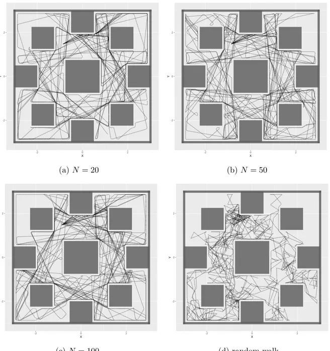
Foa score distribution for N = 20 has a lower mean than the ones with N = 50 and N = 100. All RBNs distributions are generally much worse than the random walk distribution. In fact for obstacle avoidance task random walk is a strategy often taken into account, at least as a benchmark for other options. However the fittest RBNs are capable of getting higher score than random walk. Through visual inspection robots that have a score equal to or higher than 0.05 do not get stuck and run almost a third of the arena.

Computing the Wilcoxon’s test on fitness values between RBNs with different nodes number we obtain the result in table 5.1. Using a confidence level of 0.99 we have to reject the null hypothesis when we compare networks with N = 20 and N = 50 and networks

(46)

5.1 Obstacle Avoidance 31

Figure 5.1: Foa score distributions. From left to right distributions for: RBNs with N = 20, N = 50, N = 100 and random walk controller. Each distribution counts 1000 experiments.

N value

p-value

reject H

0

20 - 50

7.0785e-13

yes

20 - 100

7.0845e-16

yes

50 - 100

0.3806

no

Table 5.1: p-value results of Wilcoxon’s test applied to Foa score of networks grouped by nodes number in obstacle avoidance. Confidence is set equal to 0.99.

with N = 20 and N = 100. This means that the number of nodes is a parameter that has statistically influence on the probability of getting a better RBN for obstacle avoidance task. We cannot reject the null hypothesis in the case of N = 50 and N = 100, there is no statistically difference between the two distributions.

In figure 5.2 is reported a qualitative performance appearance of 20 robots that have obtained the highest scores per controller category. Top RBNs behave similar to each

(47)

other, while top random walk controllers tend to explore less.

(a) N = 20 (b) N = 50

(c) N = 100 (d) random walk

(48)

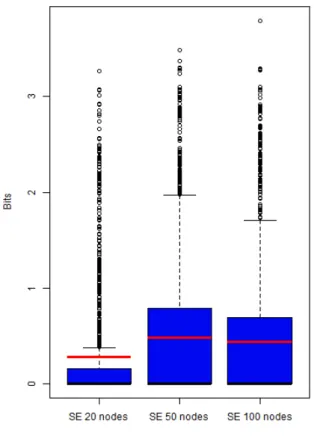
5.1.2 Measures

Measures distributions are illustrated in figures 5.3 and 5.4. Qualitative speaking, besides SE, all measures have the majority of values near zero. We explain higher medians and means for SE because this measure concerns only sensors and has an higher full scale (8 bits instead of 2). Robots that perform the task sufficiently well see in the course of the experiment more distinct sensor values than the others. Seeing more sensor values means that the probabilities tend to be more evenly distributed across all possible values and this increases the entropy. The other measures instead consider also the actuators, in particular the information relation between sensors and actuators. However the nature of obstacle avoidance affects the bound between the two: robot’s movement is altered by obstacles and perimeter walls and this leads to low metrics.

Figure 5.3: SE score distributions for obsta-cle avoidance. Distributions are grouped by node number: N = 20, N = 50, N = 100. Each distribution counts 1000 experiments.

(49)

Figure 5.4: Measures score distributions without SE for obstacle avoidance. From left to right distributions for PI, TE and RTE. Distributions are grouped by node number: N = 20, N = 50, N = 100. Each distribution counts 1000 experiments.

5.1.3 Correlation

Pearson’s correlations values are reported in table 5.2.

Nodes Foa - SE Foa - PI Foa - TE Foa- RTE

correlation p-value correlation p-value correlation p-value correlation p-value 20 0.7675 5.1963e-195 0.5129 3.4324e-68 0.4616 6.1912e-54 0.3054 4.8483e-23 50 0.7913 1.608e-215 0.5193 3.7366e-70 0.4291 4.4539e-46 0.1745 2.7753e-08 100 0.8027 2.4937e-226 0.5725 3.6817e-88 0.3762 5.524e-35 0.1581 5.0006e-07

Table 5.2: Pearson’s correlations between information theory measures and Foa. Results are grouped by nodes number and each of them refers to 1000 experiments.

(50)

SE

First thing to notice is that SE shows a strikingly high positive correlation with the objective function. For all N values correlation is higher than 0.76. This is a confirmation of what anticipated in the previous section: robots suitable for obstacle avoidance see more different sensor values and therefore have higher SE.

SE - Foa plots are shown in figures 5.5, 5.6 and 5.7. We observe similar plots for all

Figure 5.5: SE - Foa plot for networks with N = 20.

network’s configurations. When SE is between 0 and 1 Foa rises in all RBNs. Also when SE grows until almost 2.5 bits Foa still continues to increase. However there are several robots that have a medium or high SE value but a medium or low objective function. Thought visual inspection we have checked the behaviour of these robots and found that they do not move too far away from the starting position. Furthermore some of them loop around an obstacle or stop moving towards the end of the experiment. Robots that have the highest values of SE, greater than 2.5, do not have the highest objective function. A theoretical explanation is that to achieve obstacle avoidance a robot should be more often in a place where it does not perceive objects nearby. So the probability for the sensors value corresponding to this scenario to appear is much higher than the

(51)

Figure 5.6: SE - Foa plot for networks with N = 50.

(52)

values for obstacles near the robot. This unbalance in the probabilities prevents robots to get very high SE score. Instead robots that loop around obstacle have more equally balance probabilities and so higher SE despite being less capable of performing obstacle avoidance given the objective function we have chosen. The column in proximity of SE = 0 refers to robots that for the whole experiment perceive no obstacles, which corresponds to the starting state. Some of them have Foa greater than 0 because they move in circle remaining close to the starting position.

Paths of the top 20 robots with respect to SE are reported in figure 5.8. Some robots

(a) N = 20 (b) N = 50 (c) N = 100

Figure 5.8: obstacle avoidance paths for top 20 robots with respect to SE.

explore almost the whole arena but also some of them loop around one or two obstacles. This last behaviour is visible at darker sections of the arena. Overall these figures are not too distant from the ones in 5.2.

PI

PI - Foa plots are shown in figures 5.9, 5.10 and 5.11. Predictive information is mildly positively correlated with Foa, correlation is between 0.51 and 0.57. All plots are pretty similar to each other. In particular we can observe that in correspondence of PI ≈ 0.4 robots reach highest values for the objective function. Instead robots that have the highest PI have medium values of Foa. These robots tend to run a circle with different radius or to bounce between two obstacles as reported in figure 5.12. Paths

(53)

Figure 5.9: PI - Foa plot for networks with N = 20.

(54)

Figure 5.11: PI - Foa plot for networks with N = 100.

(a) N = 20 (b) N = 50 (c) N = 100

Figure 5.12: obstacle avoidance paths for top 20 robots with respect to PI.

are much different with respect to the ones in figure 5.2. We can assert that PI is only partially positively correlated with the chosen objective function for obstacle avoidance. In particular this is true for moderate values of predictive information.

(55)

TE

TE is weakly positively correlated with Foa. Correlation values are between 0.37 and 0.46. TE - Foa plots are shown in figures 5.13, 5.15 and 5.16. These plots resemble

Figure 5.13: TE - Foa plot for networks with N = 20.

(a) N = 20 (b) N = 50 (c) N = 100

Figure 5.14: obstacle avoidance paths for top 20 robots with respect to TE. the previous ones for PI. There is a concentration of robots near TE ≈ 0.12 that have

(56)

Figure 5.15: TE - Foa plot for networks with N = 50.

(57)

high objective function. Above the threshold of 0.12 bits robots tend to perform worse. Robots that have highest values for TE have medium or low objective function. Paths of the top 20 robots that have highest transfer entropy are reported in figure 5.14. We observe more cycles and general less propensity to move far away from the starting point. We can assert that there is no evidence of notable correlation between transfer entropy and the chosen objective function for the task of obstacle avoidance.

RTE

RTE is not positively nor negatively correlated with Foa. Correlation values are between 0.15 and 0.30. RTE - Foa plots are shown in figures 5.17, 5.18 and 5.19. Both robots that are suited for obstacle avoidance and that are not with respect to the chosen objective function have very low value of RTE. Paths of the top 20 robots that have highest reverse transfer entropy are reported in figure 5.20. Like in TE, robots make cycles and they move less far away from the starting point. We can assert that there is no evidence of notable correlation between reverse transfer entropy and the chosen objective function for the task of obstacle avoidance.

(58)

Figure 5.18: RTE - Foa plot for networks with N = 50.

(59)

(a) N = 20 (b) N = 50 (c) N = 100

Figure 5.20: obstacle avoidance paths for top 20 robots with respect to RTE.

5.2 Path Following

5.2.1 Objective function

Fpf score distributions are summarized in figure 5.1. Like in the previous task RBNs generally perform worse than the random walk controller. This is due for the same reason as before: the majority of robots does not move or stop moving after few simulation steps. However we observe that the fittest robots according to the chosen objective function that use RBNs outperform the ones with the random walk controller. Top RBNs have Fpf higher than 4, while top random wolk robots have Fpf near 2. Through visual inspection robots that have a score equal or higher than 2.5 start to run across the path but with some inconsistency like loops. Robots with Fpf higher than 3 perform the task considerably well.

Computing the Wilcoxon’s test on fitness values between RBNs with different nodes number we obtain the result in table 5.3. Accordingly to p-values using a confidence Table 5.3: p-value results of Wilcoxon’s

test applied to Fpf score of networks grouped by nodes number in obstacle avoidance. Confidence is set equal to 0.99.

N value

p-value

reject H

0

20 - 50

1.4344e-17

yes

20 - 100

6.3114e-31

yes

50 - 100

0.0086

yes

(60)

5.2 Path Following 45

Figure 5.21: Fpf score distributions. From left to right distributions for: RBNs with N = 20, N = 50, N = 100 and random walk controller. Each distribution counts 1000 experiments.

level of 0.99 we have to reject the null hypothesis when we compare 20 and 50 nodes networks, 20 and 100 nodes networks and 50 and 100 nodes networks. This means that the number of nodes is a parameter that has statistically influence on the probability of getting a better RBNs for Path Following task, in this case with N = 50.

In figure 5.22 is reported a qualitative performance appearance of 20 robots that have obtained the highest scores per controller category. Top RBNs behave quite similar to each other (top RBNs with N = 100 are a bit worse), while top random walk robots do not achieve the objective. We observe that in RBNs paths there are some circles in correspondence of angles or wavy lines. After one or two circles robots settle and proceed over the path. Sometimes few robots cut through the circuit but ultimately when they reach it again continue to perform path following.

(61)

(a) N = 20 (b) N = 50

Figure 5.22: path following paths for top 20 robots with respect to Fpf.

5.2.2 Measures

Measures distribution are shown in figures 5.24 and 5.23. SE distributions have low medians but values reach almost 5 bits on a scale of 8. It is worth remember that it is

(62)

Figure 5.23: Measures score distributions without SE for path following. From left to right distributions for PI, TE and RTE. Distributions are grouped by node number: N = 20, N = 50, N = 100. Each distribution counts 1000 experiments.

impossible to reach too high values due to the arena configuration. The low median is explained by robots that do not move or move only for few steps. Despite the task of obstacle avoidance the other measures distributions have higher means. This is due to the fact that robots are subjected to more different stimuli rather than in obstacle avoidance where a robot perceives only if it is close to an object and only in the object’s direction. In path following a robot starts on the circuit and because the lines are generally not too wide and cover the nearby robot space there is an high variety of sensor values. Therefore robot’s movement is not affected except from the external walls.

5.2.3 Correlation

(63)

Figure 5.24: SE score distributions for path following. Distributions are grouped by node number: N = 20, N = 50, N = 100. Each distribution counts 1000 experiments.

Fpf - SE Fpf - PI Fpf - TE Fpf - RTE

correlation p-value correlation p-value correlation p-value correlation p-value

20 0.5594 2.0326e-83 0.7148 3.3282e-157 0.8513 6.7828e-282 0.7717 2.078e-198

50 0.5089 5.4219e-67 0.735 1.2622e-170 0.7897 4.9862e-214 0.7749 4.5517e-201

100 0.4184 1.1752e-43 0.6807 4.2987e-137 0.7669 1.6546e-194 0.74 4.2484e-174

Table 5.4: Pearson’s correlations between information theory measures and Fpf. Results are grouped by nodes number and each of them refers to 1000 experiments.

SE

SE unlike in the obstacle avoidance task is not the most correlated measure with Fpf. Indeed it is the less correlated, but correlation values are not too low, range is between 0.41 and 0.55. SE - Fpf plots are shown in figures 5.25, 5.26 and 5.27. From 0 to 2 bits Fpf increases, however there are several robots that have high SE and objective

(64)

Figure 5.25: SE - Fpf plot for networks with N = 20.

(65)

Figure 5.27: SE - Fpf plot for networks with N = 100.

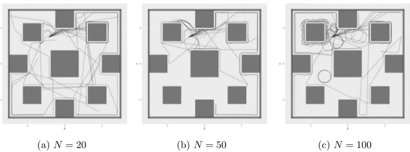
function still near to 0. From a theoretical prospective to maximize SE a robot has to perceive different sensor values with equal probabilities. This behaviour is achieved by robots that move in circle around the path. Paths of the top 20 robots with respect to SE are reported in figure 5.28. We observe robots performing roto-translation over the

(a) N = 20 (b) N = 50 (c) N = 100

Figure 5.28: path following paths for top 20 robots with respect to SE. path corresponding to darker areas or rings in the plots.

(66)

After this deeper investigation we assert that despite SE has a moderate positive value of correlation with the chosen objective function robots with the highest SE do not perform well in path following task.

PI

PI has correlation values between 0.68 and 0.73 with Fpf. This indicates that the metric is positively correlated with the chosen objective function. PI - Fpf plots are shown in figures 5.29, 5.30 and 5.31. We notice that generally robots with higher PI

Figure 5.29: PI - Fpf plot for networks with N = 20.

have higher score, however a notable number of robots with medium or high metric have medium or low score. Through visual inspection we have found that for these robots Fpf is not high because they run the same section path more time back and forth. So they do not reach far positions from the starting one and consequentially do not get high score. High value of correlation for predictive information is explainable by the fact that a robot, to stay on the path while moving, must have its actuators well coupled with its sensors. The RBN that controls the robot “recognizes” when to turn right or left based on the sensor values. Otherwise a robot cannot follow the path and gets a low score.

(67)

Figure 5.30: PI - Fpf plot for networks with N = 50.

(68)

Robots that instead have low PI and medium or high Fpf have less smooth movements with swings while running a straight line. Paths of the top 20 robots with respect to SE are reported in figure 5.32.

(a) N = 20 (b) N = 50 (c) N = 100

Figure 5.32: path following paths for top 20 robots with respect to PI.

TE

TE is strongly positively correlated with Fpf. Correlation goes from 0.76 to 0.85 and it is the highest of the four. TE - Fpf plots are shown in figures 5.34, 5.35 and 5.36.

(a) N = 20 (b) N = 50 (c) N = 100

Figure 5.33: path following paths for top 20 robots with respect to TE.

(69)

Figure 5.34: TE - Fpf plot for networks with N = 20.

(70)

Figure 5.36: TE - Fpf plot for networks with N = 100.

with medium or high TE and medium or low score. The ones that still persist can be explained with the same reason: robots do not reach far positions. Also robots that have medium TE and high Fpf behave like the ones in PI. Paths of the top 20 robots with respect to TE are reported in figure 5.33. We notice a clear similarity with figure 5.22. In this case there are a bit more circles, especially in proximity of tight curves of the circuit.

After this deeper analysis we assert that transfer entropy from sensors to actuators is strongly positively correlated with the chosen objective function for the task of path following. TE can definitely be used as an alternative objective function that is not handcrafted by humans.

RTE

RTE is strongly positively correlated with Fpf and has similar values of TE, it goes from 0.74 to 0.77. RTE - Fpf plots are shown in figures 5.37, 5.38 and 5.39. We observe a solid logarithmic grow of the objective function. There are no robots with high RTE and low score, robots with more than 0.2 bits are all suitable for path following. Paths of

(71)

Figure 5.37: RTE - Fpf plot for networks with N = 20.

(72)

Figure 5.39: RTE - Fpf plot for networks with N = 100.

the top 20 robots with respect to RTE are reported in figure 5.40. Paths are extremely close to the ones in figure 5.22.

(a) N = 20 (b) N = 50 (c) N = 100

Figure 5.40: path following paths for top 20 robots with respect to RTE.

Ultimately the transfer entropy from actuators to sensors is a metric strongly posi-tively correlated with the chosen objective function. It can be used as an alternative not handcrafted objective function for the path following task.

(73)

5.3 Phototaxis

5.3.1 Objective function

F pt score distributions are summarized in figure 5.41. Differently from the previous

Figure 5.41: Fpt score distributions. From left to right distributions for: RBNs with N = 20, N = 50, N = 100 and random walk controller. Each distribution counts 1000 experiments.

tasks, the chosen objective function for phototaxis is not limited by 0. A standing robot get almost a score of 0.2727. A robot that moves away from the light source gets a lower value. We notice that both RBNs and random walk controller have similar means and medians. However the most suitable RBNs outperform the best random walk robots. With Fptgreater than 0.4 robots move towards the light source but not in the fastest way. Not all robots with score close to 0.4 ends nearby the light source, but they definitely reduce the distance. Robots that get a score higher than 0.45 end in close proximity of

(74)

5.3 Phototaxis 59

the light source. With more than 0.5 robots go straight forward towards the light source.

(a) N = 20 (b) N = 50

Figure 5.42: phototaxis paths for top 20 robots with respect to Fpt.

An information theory analysis of critical Boolean networks as control software for robots