Alma Mater Studiorum - University of Bologna
School of Engineering
Department of Industrial Engineering Second-cycle Degree in Mechanical Engineering
Master degree thesis in
Modeling and Control of Internal Combustion Engines and Hybrid Propulsion Systems M
Development of a speed profile prediction
algorithm based on navigation data for energy
management optimization
Candidate
Mattia Boccolini
Advisor
Prof. Nicol`o Cavina Co-Advisors
Ing. Alessandro Perazzo Ing. Lorenzo Brunelli
Ing. Alessandro Capancioni Prof. Davide Moro
Prof. Enrico Corti
Alma Mater Studiorum - Universit`
a di Bologna
Scuola di Ingegneria
Dipartimento di Ingegneria Industriale
Corso di Laurea Magistrale in Ingegneria Meccanica
Tesi di laurea in
[Modeling and Control of Internal Combustion Engines and Hybrid Propulsion
Modeling and Control of Internal Combustion Engines and Hybrid Propulsion
Systems M
Development of a speed profile prediction
algorithm based on navigation data for energy
management optimization
Candidato
Mattia Boccolini
Relatore
Prof. Nicol`o Cavina
Correlatori
Ing. Lorenzo Brunelli
Ing. Alessandro Capancioni Ing. Alessandro Perazzo Prof. Davide Moro Prof. Enrico Corti
La somma delle radici quadrate di qualunque due lati di un triangolo isoscele
`
e uguale alla radice quadrata del rimanente.
[Scarecrow
Abstract
During the last decades the number of vehicles on the roads progressively rises together with the relative emissions of pollutants, such as CO2 and other green-house gases, worsening air quality and traffic conditions especially in metropolitan areas. The OEM (Original Equipment Manufacturer) are investing a lot of money in alternative solutions, progressively abandoning the Internal Combustion Energy which can no longer satisfy the more and more stringent regulations as well as the market requests. The general tendency is to introduce an alternative source of energy flanking the conventional engine, allowing its downsizing and helping it during the less efficient operating points. Moreover, the new kind of sensor systems (named Advanced Driver-Assistance Systems) are starting to be implemented on-board in addition to connectivity devices. From this union, a connected vehicle arise, able to exchange data with the surrounding environment and give the driver new kind of assistance functionality, like the Lane Departure Warning, Adaptive Cruise Control and Parking Assistance, avoiding dangerous or inefficient decisions. In parallel, these functions can recreate an electronic horizon, based on the path selected by the driver, supplying to the Control Unit a detailed preview. The natural tendency is to gradually limiting the driver control on the vehicle up to definitely excluding him from driving decisions. Nevertheless, the implementation of fully working and safe ADAS functions implies millions of kilometres of road test validations, to safely introduce them on the market. Thus, the OEM have to develop new methodologies to substitute the road tests with specific simulations, where tools (like Model-in-the-Loop, Software-in-the-loop, Hardware-in-the-Loop) are used to verify its reliability. This master thesis work wants to develop and implement an on-board algorithm for the speed prediction of a connected vehicle along a given route, by elaborating real-time navigation data. In particular, information about the legal speed limits, the
and roundabouts, are sent to the vehicle by the map service provider and they constitute the input for the algorithm. The algorithm allows you to select one out of three different driver type (quiet, normal, aggressive): this choice, together with the performance parameters of the vehicle, influences the acceleration and braking phases of the prediction. Once the prediction is generated, it constitutes an input for the predictive ADAS functions and energy management functions. The work has been split in three main phases: development, calibration end validation. During the first phase, the logics of the algorithm have been implemented by means of a Simulink block in order to be included into the Hybrid Control Unit at the HiL. Sub-sequently, the calibration of the key parameters took place by means of real speed profile analysis. In the end, the behaviour of the algorithm has been investigated studying its response in different scenarios.
The master thesis activity has been carried out at Green Mobility Research Laboratory, born by the collaboration between the University of Bologna and FEV Italia s.r.l, internationally recognized leader in design and development of advanced gasoline, diesel and hybrid powertrains and vehicle systems.
Abstract in lingua italiana
Negli ultimi decenni si `e registrato un progressivo aumento dell’utilizzo di mezzi di trasporto individuali e delle relative emissioni di agenti inquinanti, come CO2 e altri gas serra, peggiorando la qualit`a dell’aria e la viabilit`a, specialmente nelle aree metropolitane. Le case costruttrici stanno investendo molte risorse in soluzioni alternative, riconoscendo come i motori a combustione interna, per quanto efficienti questi possano essere, non riescano pi`u a soddisfare le richieste di mercato e ri-spettare la legislazione sempre piu stringente. L’obiettivo dichiarato `e l’abbandono graduale dei combustibili fossili in favore di una progressiva elettrificazione dei vei-coli. L’implementazione di una fonte di energia alternativa, in particolare quella elettrica, permette una riduzione delle dimensioni del motore termico e un aiuto nei punti operativi meno efficienti ma richiede una nuova concezione della sua gestione a bordo. In pi`u, l’istallazione nel veicolo di nuovi sistemi di sensoristica avanzata (in gergo Advanced Driver-Assistance Systems) e di moderni dispositivi di connectivity, lo rendono capace di comunicare con l’ambiente circostante, aprendo all’introduzio-ne di nuove funzionalit`a di supporto al guidatore, come il Laall’introduzio-ne Departure Warning, Adaptive Cruise Control e Parking Assistance, per evitare che esso compia scelte pericolose o inefficienti. Parallelamente queste funzioni possono permettere la ri-costruzione di un orizzonte elettronico, basato sul percorso deciso dal guidatore, fornendone alla centralina un’anteprima dettagliata. La conseguenza naturale sa-ra quella di limitare progressivamente il controllo del guidatore sul veicolo fino ad escluderlo definitivamente. Tuttavia, l’implementazione di funzionalita ADAS pie-namente funzionanti e sicure prevedrebbe milioni di chilometri di test su strada, prima di introdurle sul mercato. Ci`o obbliga i costruttori a sperimentare nuove ti-pologie di validazione per soddisfare questa esigenza sostituendo i test stradali con
the-Loop, Software-in-the-Loop, Hardware-in-the-Loop) per verificarne l’affidabilita. Questo elaborato si pone l’obbiettivo di implementare un algoritmo on-board per la predizione della velocit`a di un veicolo connesso, lungo un dato percorso, per mezzo dell’elaborazione dei dati di navigazione real-time. In particolare, le informazioni riguardanti i limiti di velocit`a, la densit`a di traffico e la presenza di eventuali ”stop events” come semafori e rotonde, vengono inviate al veicolo dal map service pro-vider e costituiscono gli input dell’algoritmo. L’algoritmo permette di scegliere tra tre diversi tipi di driver (prudente, normale, aggressivo): questa selezione, insieme ai parametri di prestazioni del veicolo pre-impostati, andr`a ad influenzare le fasi di accelerazione e decelarazione nella predizione. Una volta generata, tale predizio-ne costituisce l’input delle funzioni ADAS predittive e di quelle addette all’epredizio-nergy management. Il lavoro `e stato suddiviso in tre fasi principali: sviluppo, calibrazione e validazione. Durante la fase di sviluppo, le logiche dell’algoritmo sono state im-plementate in Simulink in modo da poter essere inserite nell’ Hybrid Control Unit (HCU) del Software-in-the-Loop. Successivamente, `e stata effettuata la calibrazio-ne dei paramentri principali dell’algoritmo, basata sull’analisi di profili di velocit`a acquisiti su strada. Infine, `e stata investigata la risposta dell’algoritmo a scenari diversificati.
Il lavoro di tesi `e stato svolto presso il Green Mobility Research Laboratory, nato dalla collaborazione tra l’Universit`a di Bologna e FEV Italia s.r.l., compagnia internazionale leader nella progettazione e nello sviluppo di powertrain e sistemi veicolo.
Acknowledgments
My heartfelt thanks to Professor Nicol`o Cavina, who has given me the opportu-nity to start this formative project, but above all for letting me understand what I want to do when i grow up. Another special thanks to Ing. Alessandro Capancioni and Lorenzo Brunelli for guiding me during the whole project. I cannot omit to thank all the FEV Bologna team, for welcoming me and for making me feel part of it from the first day. Lust but not least, I have to say thank you to Denise and Rebecca for giving me a ride to the laboratory every day, and to Giorgio for being my ”driver type: normal” during the measurements.
Contents
Abstract ix
Abstract in lingua italiana xi
Acknowledgments xiii
List of figures xvii
List of tables xix
Nomenclature 1
1 Introduction 1
1.1 Motivations, challenges and targets . . . 1
1.2 ADAS . . . 8
1.3 Connectivity . . . 10
1.3.1 Predictive driving (eHorizon) . . . 11
2 Simulation environment 15 2.1 Simulation environment . . . 15
2.2 Model-in-the-Loop . . . 16
2.3 Software-in-the-Loop . . . 17
2.4 Connected Hardware-in-the-Loop . . . 19
3 Speed Profile Prediction 21 3.1 State of the art . . . 21
3.3.1 Traffic density . . . 24
3.3.2 Stop events . . . 25
3.3.3 Space based driver model . . . 27
3.3.4 Oscillation around constant speed segments . . . 29
4 Calibration procedure 33 4.1 Methodology . . . 33
4.1.1 Scenarios . . . 33
4.1.2 Measurements . . . 35
4.1.3 Key Performance Indicators . . . 37
4.2 Calibration . . . 39
4.2.1 Acceleration and braking maneuvers . . . 40
4.2.2 Traffic: influence on average speed and oscillations . . . 40
5 Results and validation 45 5.1 Scenario 1 . . . 45
5.2 Scenario 2 . . . 47
5.3 Scenario 3 . . . 50
6 Conclusions and future works 53 6.1 Initial and final speed . . . 53
6.2 Oscillation energy . . . 54
6.3 Road curvature radius and weather conditions . . . 55
6.4 Stop event duration, slope and eco-Driving . . . 56
List of figures
1.1 Overview of the Hybrid Electric Vehicle depending on Hybridization
and CO2 reduction . . . 4
1.2 Fuel specific energy in function of their volumetric density . . . 5
1.3 Parallel hybrid power characteristics . . . 5
1.4 Series/Parallel hybrid power characteristics . . . 6
1.5 Series hybrid power characteristics . . . 6
1.6 Parallel hybrid driveline architecture . . . 7
1.7 On-board sensing equipment . . . 9
1.8 Automation levels according to SAE . . . 10
1.9 V2X connectivity . . . 11
1.10 Ideal predictive strategy . . . 12
1.11 Zero Emission Zone . . . 13
2.1 V-Model methodology layout . . . 16
2.2 Software-in-the-Loop scheme . . . 18
3.1 Previous version of the speed profile prediction . . . 23
3.2 Green traffic light probability depending on traffic code. . . 26
3.3 Verified conditions for acceleration. . . 28
3.4 Effects of different τ = 1 T in a first order system undergoing to a step stimulus. . . 29
3.5 Measured speed profile Vs. ”zero-noise” predicted speed profile . . . . 30
3.6 Measured speed profile Vs. Predicted speed profile . . . 31
brakis, Bologna . . . 35
4.3 Measurement chain . . . 36
4.4 u-center GUI: speed over time diagram view . . . 36
4.5 u-center GUI: table view with time, speed, longitude and latitude . . 36
4.6 Acceleration and braking: before(left) and after(right) calibration . . 40
4.7 Example of FFT applied to a distance-based measured signal . . . 41
4.8 Frequency and magnitude’s scatter in case of traffic code ’orange’ . . 43
5.1 Scenario 1: speed . . . 46 5.2 Scenario 1: energy . . . 47 5.3 Scenario 2: speed . . . 48 5.4 Scenario 2: energy . . . 49 5.5 Scenario 3: speed . . . 51 5.6 Scenario 3: energy . . . 51
6.1 Effects of oscillations on KPI . . . 54
6.2 Limit of adherence C . . . 56
List of tables
3.1 SPP input . . . 24
3.2 Stop event typologies . . . 25
4.1 Calibration parameters . . . 39
5.1 Scenario 1:speed KPI . . . 45
5.2 Scenario 1:energy KPI . . . 46
5.3 Scenario 2:speed KPI . . . 47
5.4 Scenario 2:energy KPI . . . 48
5.5 Scenario 3:speed KPI . . . 50
Chapter 1
Introduction
1.1
Motivations, challenges and targets
Starting from the twentieth century, the population growth, together with the technological development, has lead the industrialization process to completely new scenarios: the birth of more and more factories and the consequent movement of the people from the countryside to the city centres. This period saw an exponen-tial growth of production, giving the people technologies, once prohibitive for the price and now more accessible. As a natural consequence of the economic boom, in parallel with a general carelessness and incompetence about environment, the emissions of carbon dioxide (CO2) and other greenhouse gases (GHG) rapidly in-creased over the year, becoming one of the most challenging issues of the present time. An important role is played by the automotive industries, in fact, cars are used throughout the world and they have become the most adopted solution for people transportation in many countries. Transportation was responsible for 24% of direct CO2 emissions in 2017. The 77% of both global final energy demand and CO2 emissions are accountable to the transport sector as a whole, comprehending cars, trucks, buses and two-wheelers. Moreover, car buyers continue to choose big-ger, heavier vehicle and this has lead to a rise in the average new car CO2 emissions in 2017 [1]. Therefore, the European Union has made substantial efforts tightening the CO2 maximum limit on a Worldwide harmonized light vehicles test procedure from 130 gCO2/
gCO2/
km by 2030 [10]. Hence, automobile manufacturers and engineers have spent the last decade trying to develop innovative solutions with the double purpose of satis-fying the market request and complying to the regulations, increasingly stringent. The result of these years of research is the decision to adopt other form of energy supporting the conventional engine. In the so-called Hybrid Vehicles the primary energy source is generally an Internal Combustion Engine (ICE); depending on the nature of the secondary source, ”Hybrid” can mean
Hydraulic Hybrid that kind of vehicles have a hydraulic pump as secondary mover or generator, which stores the energy in an auxiliary hydraulic accumu-lator where oil is used as operator fluid. For their weight and their character-istics, this powertrain is particularly indicated for heavy-duty vehicles;
Kinetic Hybrid kinetic hybrid powertrain means a driveline with a highspeed flywheel as auxiliary mover, with the possibility of storing kinetic energy, es-pecially during regenerative braking; [6]
Compressed-air Hybrid these vehicle are powered by motors which produce power with the compressed-air expansion in a similar way of the steam engine. As a non-flammable fluid, the compressed-air can be stored in pressurized tank at 30 MPa;
Electric Hybrid here, the auxiliary energy source is the electro-chemical energy provided by Electric Motors and the batteries are the storage system which can be recharged during breaking or with the ICE.
The more promising technology in term of CO2 reduction is the Hybrid Electric Vehicle (HEVs). Focusing on them, the level of hybridization depends on the range of action of the electric motor which is indicated by the Hybridization Degree (HD) and described by the eq.(1.1)
HD= PS,max PS,max+ PICE,max
(1.1)
1.1 – Motivations, challenges and targets
is the maximum power deliverable by the ICE. Consequently, it is possible to dis-tinguish the following typology of HEVs:
Micro Hybrid with a HD ∼ 5%, it’s a vehicle equipped with an Electric Mo-tor (EM) linked to the ICE and it can only have Start and Stop functionality. Most of the them have also some sort of Energy Management function, which optimizes the consumption of the low voltage (12 V) battery energy [26];
MHEV (Mild Hybrid EV) with a HD ∼ 15%, these types generally use a compact electric motor (usually < 20kW ) to provide auto-stop/start features, extra power assist during the acceleration and to work as a generator on the deceleration phase (regenerative braking). The battery is a Low Voltage Bat-tery of 48V, whose purpose is to actuate an Energy Management Strategy (EMS) and it allows a minimum range of full-electric drive1.
FHEV (Full Hybrid Electric Vehicle) where the HD ∼ 35%, the Electric Ma-chines and batteries are increased in size, allowing an extended full-electric drive. The recharging of the batteries can happen only with breaking recuper-ation and with the ICE, because it isn’t possible to do from external sources;
PHEV (Plug-in HEV) is usually a general fuel-electric Off-Vehicle Charging (OVC) hybrid vehicle with increased energy storage capacity and a HD ∼ 50%. This allows the vehicle to drive on all-electric mode a distance that depends on the battery size and its mechanical layout (series or parallel). At the end of the journey, it may be connected to mains electricity supply through a socket to avoid recharging using the on-board internal combustion engine. This concept is attractive to those seeking to minimize on-road emissions by avoiding - or at least minimizing - the use of ICE during daily driving. As with pure electric vehicles, the total emissions saving, for example in CO2 terms, is dependent upon the source of the energy produced by the provider company;
BEV (Battery EV) are vehicles where there isn’t an ICE and the traction is granted only by electric motors powered by batteries. Properly, they’re not
1Exceptions of full-electric drive vehicle equipped with a 48V battery are the MEET model
hybrid vehicle, because the energy source is only one, but it will be the arrival point of the transaction where the hybrid vehicles are only intermediate step. At the moment, the main problem of BEV is the capacity of the battery cells, so how the energy is stored [26]. In Fig. 1.2, the fuel (gaseous and liquid) and batteries specific energy is represented in function of their volumetric density, there the problematics of the batteries compared to the other fuels are clearer. To make a more practical example, the same energy needed for a drive of about 500km is stocked in 46 litres (∼ 43kg) of gasoline but in more than 700kg of batteries. Nevertheless, from the dawn of the batteries for automotive purpose, thanks to the improvement in technology their cost becomes cheaper and cheaper, while their energy density increases [21].
Figure 1.1: Overview of the Hybrid Electric Vehicle depending on Hybridization and CO2
reduction
Once the typology has been defined, it is possible to describe how the energy flow is transferred from the energy storage (tank for ICE or battery for the EMs) to the wheels. Three paths are possible:
1.1 – Motivations, challenges and targets
Figure 1.2: Fuel specific energy in function of their volumetric density
assistance as needed, delivering torque from zero rpm during standing starts and acceleration. This cooperation consent to avoid engine working points where the specific fuel consumption is high. The powertrain can be adapted simply by adding an electric motor and batteries to an existing vehicle, as in Fig. 1.3.
Figure 1.3: Parallel hybrid power characteristics
parallel layouts. In particular, the EM powers the vehicle from a standing start and at low speed whereas, as the speed increases, ICE and EM work together to efficiently provide the power required. As can be expected, the system is more complex featuring a power split device and a generator. An exemplification is shown in Fig. 1.4.
Figure 1.4: Series/Parallel hybrid power characteristics
Series the series layout provides torque solely by using electric motors, like electric vehicles, and the aim of ICE is to recharge the battery with the gen-erator. The powertrain is equivalent to an EVs, but because the vehicle also includes an engine, it is considered a hybrid (Fig. 1.5) [8].
Figure 1.5: Series hybrid power characteristics
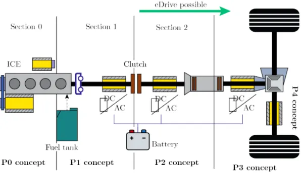
For what concern the HEVs parallel topology, several architectures are possible differing from each other for the position of the electric machines within the driveline. As shown in Fig. 1.6, they are as follow:
P0 the engine is coupled to the motor through a belt, so the electric machines is called Belt-driven Starter Generator (BSG);
1.1 – Motivations, challenges and targets
P1 the EM is directly mounted on the crankshaft, upstream of the clutch, and it is named Integrated Starter Generator (ISG);
P2 the EM is separated from the engine by a clutch, that allows the pure electric drive;
P3 the EM is mounted on the secondary shaft out of the gearbox;
P4 the EM is connected to the front or rear wheels by means of a transmission ratio;
Figure 1.6: Parallel hybrid driveline architecture
Introducing a different type of energy flow (electrical energy) additional to the chemical one, engineers have to face new challenging problems. In fact, while the available space remains the same, the components rise in number: one or more elec-tric motors, a bigger battery, a more powerful control unit and the inverters have to be rationally placed inside the vehicle. Adding new components doesn’t imply only a different spacing configuration but it also means a more complex control at system level and also regarding the safety. On one hand, it’s possible to achieve sim-ilar performance to standard vehicle with internal combustion engine while greatly
improving fuel efficiency and tailpipe emission, recovering the energy from braking. On the other hand the torque split (so how the torque request is fulfilled) becomes the new control variable and it is complicated to handle. The challenge is to find the more efficient split that covers the torque request among the possible solutions. As a matter of fact, the computational effort of the control unit becomes heavier. Finding the optimal or sub-optimal solution is a part of the so called Energy Management Strategy which tries to minimize a two-variables function, where the fuel consump-tion is no longer the only parameter to keep under observaconsump-tion, but it’s flanked by a new one: the state of charge of the Battery Storage System, shortened SoC. The state of charge represents the actual capacity of the battery over its maximum ca-pacity and it’s expressed in percentage. To better understand its meaning, it could be compared to the physical level of the liquid fuel in the tank. So then, the OEMs have invested money and time to develop new energy optimization strategies with the purpose of minimizing the overall energy consumption.
1.2
ADAS
The general tendency is moving toward a vehicle efficient and clean, but a non-negligible limit to that goal it will always be the driver, the less predictable variable in the system. The innovative Advance Driver-Assistance Systems (ADAS) come to help limiting the driver actions but they require a reliable detection of the vehicle and the surrounding environment. That virtual reconstruction permits the Hybrid Control Unit (HCU) to make more efficient choices both regarding the road safety as well the torque management. The new generation of on-board sensors and control strategies assist a common driver during acceleration and braking and they help him avoiding inefficient decisions such as during the gear shift, stop & start sys-tem, increasing the driving comfort and safety. A short explanation of that kind of equipment is given below, and it is shown in Fig. 1.7.
LIDAR (LIght Detection And Ranging)
remote sensing method that uses light in the form of a pulsed laser to measure ranges (variable distances) [20].
1.2 – ADAS
detection system that uses radio waves to determine the range, angle, or veloc-ity of objects. In particular it is distinguished in long range (LRR) for Adaptive Cruise Control, medium range (MRR)for cross traffic alert and lane change assist, short-range (SRR) for parking aid, obstacle/pedestrian detection [12].
CAMERAS
a video sensor used to perceive the environment around the vehicle.
Figure 1.7: On-board sensing equipment
All these efforts are made with the aim of designing and producing an autonomous vehicle capable of driving safely and efficiently on the road. This, from one hand will erase or at least reduce mortal accidents, and on the other hand will gave to the people a less polluting way of transportation. Obviously, to reach that goal, some gradual steps have to be fulfilled. The Society of Automotive Engineers (SAE) has defined different automation levels, which span from Level 0, without automation systems, to Level 5, where the car is completely self-driving [14]. In Fig.1.8 there is represented a schematic description of each level. In the future, the ADAS will intervene in the driving process more intensively and autonomously, for example
influencing braking and steering maneuvers (with traffic jam chaffeur or motorway autopilot functionalities) [9].
Figure 1.8:Automation levels according to SAE
1.3
Connectivity
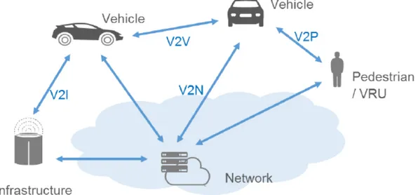
The way toward the autonomous driving is strictly linked with the progresses made by the telecommunication industries, in a on-going development of the Vehicle-to-Everything (V2X) connectivity technologies, with the aim of passing information from a vehicle to any entity that may affect the vehicle and vice versa:
Vehicle-to-Vehicle (V2V) Vehicle-to-Infrastructure (V2I) Vehicle-to-Cloud (V2C)
Vehicle-to-Pedestrian (V2P)
The amount of information work together in order to achieve road safety, traffic efficiency and energy savings. Some of the functionality given by the connectivity could influence the vehicle as a warning (for forward collisions, lane change and
1.3 – Connectivity
blind spots) or directly acting on it. Not only they will be at the base for the optimal safety and effective autonomous driving of tomorrow, but they constitute a powerful instrument that can already be used to fill the gap introduced by the human factor. The focus of this essay, for example, is on a PHEV vehicle made connected (enabled to the V2X communication) so that it is able to exchange data with a Map Service Provider (MSP) and to use this information to forecast the driving cycle performed by the human driver. Then, this prediction named eHorizon, can be used not only by the ego-vehicle for the energy management, but it can also be shared with other users to actuate strategies of intelligent mobility.
Figure 1.9: V2X connectivity
1.3.1
Predictive driving (eHorizon)
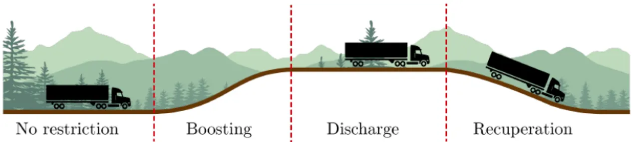
In term of efficiency, the optimal solution will be reached with the complete knowledge of the future, because it would permit to elaborate a strategy suitable for the specific route. In the following paragraph there is a very didactic example, but also very clear, of how the predictive drive will help: Fig. 1.10 shows a possible path of a commercial vehicle that approaches a climb. In normal conditions, climbing the hill, the internal combustion engine will provide the requested torque, but doing so
it recharges, or doesn’t discharge the battery. Once the car reaches the top of the climb, there is a downhill in front of it where it could perform regenerative breaking but the battery capacity could be already at the maximum limit. So the potential energy of the slope is useless. But if the presence of this difference in height were known, the control unit will allow the EMs to help the ICE during the climb, making it working at more efficient points, and at the top of the hill the battery could be recharged. This is only a little example of the enormous potential of a predictive strategy, in fact, it will be possible to avoid traffic congestions, accidents, dangerous situations and so on.
Figure 1.10: Ideal predictive strategy
This master thesis can be considered as a branch of a wider previous project developed by Green Mobility Research Laboratory (GMRL) [3] regarding predictive functions for energy management. The aim of the study was the development of these functions followed by their implementation in a parallel PHEV model (MiL) by means of Simulink [4]. In the first stage, torque management strategies have been implemented in the Control Unit in order to determine the optimal (Discrete Dynamic Programming)(DDP) or sub-optimal (Equivalent Consumption Minimiza-tion Strategy) (ECMS) torque split, as the solution of a cost function minimization problem. In this case, the cost function is the equivalent consumption of fuel (both chemical and electric). In parallel, two specific Predictive Functions (PF) have been implemented: the Zero Emissions Zone (ZEZ) and the Predictive Thermal Manage-ment (PTM)[5]. Both the functions are based on the knowledge of the driving cycle at priori. In particular, they are focused on the urban zone where the usage of the conventional engine is forbidden, so the vehicle has to switch to full electric mode. Firstly, the connectivity check if any part of the selected route belongs to a ZEZ
1.3 – Connectivity
and, in case of positive answer, the two functions are called. The Zero Emissions Zone function gives to the torque strategies a target to fulfill, in order to guaran-tee enough battery state of charge at the beginning of the event [fig.??]. On the other side, the Predictive Thermal Management decides if there is the possibility of managing the battery cooling circuit more efficiently and saving energy. In the end, the simulations results are made compliant with the newest regulations of the laboratory tests (Worldwide harmonized Light vehicle Test Cycle) and of the road tests (Real Driving Emissions).
Chapter 2
Simulation environment
2.1
Simulation environment
This chapter wants to provide an overview on the main steps that characterized the development of the Speed Profile Prediction algorithm (SPP), starting from the definition of the specifications and concluding with the implementation at the con-nected HiL. In addition, a brief description of the various adopted software/hardware architectures is presented.
It is important to stress how the whole procedure has been driven by the V-Model methodology of software development. In fact, while on the one hand the usage of connected vehicles represents a solution to crucial issues such as pollution and con-gested urban centers, on the other hand, the development of such a complex frame-work collides with the common goal of shortening the vehicle time-to-market. The old consolidated methodologies (reliable road tests above all) does not fit anymore because the safety validation of a current driver assistance system alone requires up to 2 millions test kilometers. In addition, most of the situations under control regard dangerous and highly-variable test conditions. Thus, the tendency is to move all the driven kilometers from the roads to advanced simulation environment in a process called ”from-road-to-rig-to-desktop”[3].
Figure 2.1: V-Model methodology layout
2.2
Model-in-the-Loop
The project started with the qualitative outlining of the information that could have been received from the MSP. In parallel, a bibliographic research has been con-ducted in order to define the state of the art and to assume adequate specifications as target for the logics to be implemented. Once the specifications have been clarified, the code writing phase has begun. The V-Model expects a testing procedure for each development step of the algorithm, that’s why the first version of the algorithm has been written as a script in MATLAB1: this solution allows a quick implementation of the basic logics followed by a preliminary check of their congruence and validity. Once the algorithm has passed this first test, the second step was the conversion of the script into a Simulink2 model by means of a Stateflow3 chart. The need to switch into Simulink environment stems from the fact that, this algorithm is going to be flashed into a Simulink-programmable HCU. Until this moment, the Speed
1MATLAB (an abbreviation of ”matrix laboratory”) is a proprietary multi-paradigm
program-ming language and numeric computing environment developed by MathWorks. MATLAB allows matrix manipulations, plotting of functions and data, implementation of algorithms, creation of user interfaces, and interfacing with programs written in other languages[23].
2Simulink is a MATLAB-based graphical programming environment for modeling, simulating
and analyzing multidomain dynamical systems. Its primary interface is a graphical block dia-gramming tool and a customizable set of block libraries. Simulink is widely used for multidomain simulation and model-based design[24].
3Stateflow (developed by MathWorks) is a control logic tool used to model reactive systems via
2.3 – Software-in-the-Loop
Profile Prediction Algorithm (SPP) as been treated as a stand alone model, without the slightest thought for the specifications imposed by the on-board implementa-tion, but just considering his results in terms of prediction. Nevertheless, thanks to this transition to Simulink, the inclusion of the SPP in the Model-in-the-Loop has become possible. MiL testing and simulation is a technique used to abstract the behaviour of a system or sub-system in a way that this model can be used to test, simulate and verify one or more component while they are still under development. In other words, referring to this project, it means that also in this early phase, an off-line co-simulation of the SPP coupled with the PF has been already possible, even if compatibility between software and hardware in the HCU was still to be verified.
2.3
Software-in-the-Loop
Once the logic have been implemented in Simulink, one step beyond along the development process can be done passing from a Model-in-the-Loop to a Software-in-the-Loop simulation. SiL makes it possible to test software prior to the initialization of the hardware prototyping phase, significantly accelerating the development cycle. It represents an environment where the under analysis hardware component (HCU in this case) is replaced by its digital twin, containing exactly the same software as the real one. In this way, SiL enables the earliest detection of system-level defects or bugs, reducing the costs of later stage troubleshooting, when the number and complexity of component interactions is greater. A schematic view of SiL architecture employed in this project is shown in fig. 2.2: Here below, the steps of the data flow are briefly depicted:
The virtual MSP sends navigation to the Telecommunication Control Unit (TeCU), in a format that is exactly the same as the one sent by the real MSP.
TeCU elaborates navigation data in order to make them compliance with the CAN line and sends them to the eHorizon reconstructor (eHR) inside the HCU. In particular, the vectors containing navigation data are fragmented in vector of lower size.
Figure 2.2: Software-in-the-Loop scheme
eHR reads data from CAN, re-builds the original information from fragments and generates input to feed the SPP.
SPP generates the predicted speed profile to be sent as input to the PF. PF apply the optimization strategies to the predicted speed profile, computing
2.4 – Connected Hardware-in-the-Loop
a SOC target and the thermal management strategy for the path. All the energies involved in calculations are retrieved by PF thanks to a Simulink model that reproduces the vehicle dynamics and its control system.
SUMO (Simulator of Urban MObility) provides the virtual scenarios where PF are tested off-line. The need for SUMO to be introduced in the loop comes from the fact that in real driving, the predicted cycle will never perfectly match the real one. Simulating scenarios in SUMO makes already possible at this stage the evaluation of the response of the PF to this error, by assuming the cycle driven by SUMO’s driver as the real one, avoiding costs and risks linked to road testing.
2.4
Connected Hardware-in-the-Loop
HiL, as stated by the name itself, provides more advanced tests on the control system, thanks to a detailed and already validated vehicle model implemented on a Real-Time PC that reproduce the physical signals of the environment. It includes sub-models for the vehicle longitudinal dynamics, the hybrid powertrain compo-nents, and their controllers. The Real-Time PC is connected to a rapid-prototyping HCU running an energy management supervisory controller where SSP and PF are included. Thus, while at the SiL it is possible to prevent failures due to program-ming incompatibility, the HiL testing allows in addition to avoid hardware-related problems such as overrunning or signal disturbances. Before the introduction of con-nectivity devices, HiL included only the hardware related to a conventional vehicle but, thanks to the work made by previous master thesis [7][11], it is possible today to execute on-line co-simulations, where the HiL receives real-time data by the MSP. Furthermore, to simulate at C-HiL that the vehicle under test is actually traveling along roads in a urban environment, the GPS signal is generated locally by a host PC in which SUMO is running.
Chapter 3
Speed Profile Prediction
3.1
State of the art
In the last four decades several studies about predicting the future speed of the ego-vehicle have been conducted since it is a necessary component of many Intelli-gent Transportation Systems (ITS) applications, in particular for safety and energy management systems. The speed prediction models state of the art can be grouped into two main categories: parametric and non-parametric. In the first category, we find algorithms where the driving task is modeled as a stimulus-response system, so, as a control problem where driver’s goal is to keep a safe distance with the vehicle in front or to pursue a target speed according to some imposed constrains (e.g. speed limits). The nomenclature is justified by the fact that in this kind of algorithms a model for the ego-vehicle and/or for the driver needs to be included by means of parameters: an example of the most advanced parameters model can be found in the ones developed to be implemented in traffic simulators (e.g. SUMO). More recently some non-parametric models have been proposed: this kind of algorithms are based on probabilistic theories such as Artificial Neural Network, Markov chains or Monte Carlo methods. The main advantages related to this class consist in allow-ing a greater flexibility in the representation of the dynamics and in beallow-ing suitable for machine learning and artificial intelligence systems. The counterpart is inherent in the probabilistic nature of these methods since they need time to acquire big data in order to generate consistent predictions. For a more detailed comparison
please refer to the study conducted by Lef`evre et al. Comparison of Parametric and Non-Parametric Approaches for Vehicle Speed Prediction [16].
3.2
Previous version
A basic version of a speed profile prediction algorithm was previously imple-mented [7] giving a chance for the predictive functions to be tested at the connected-HiL. This trivial version was able to receive only the information about the legal speed limits by MSP and then, assuming the vehicle speed to be coincident with the speed limit value, the transitions between different speed values were modulated following a constant acceleration/deceleration law. In addition, stop events and rel-ative duration were supposed (3.1). Although these predictions turned out to be inconsistent from an energetic point of view, this first version of the algorithm had allowed the telecommunication chain to be tested, marking the passage from HiL to a c-HiL, which was the main target at the time [7][11].
3.3 – Speed Profile Prediction algorithm
Figure 3.1:Previous version of the speed profile prediction
3.3
Speed Profile Prediction algorithm
This thesis work is based on the idea that the generation of a speed profile for energy management purposes might be a smart way to maximize the exploitation of navigation data that nowadays are commonly requested by the cars. Selecting the parametric approach has made possible to take this route in a relative short time and being free from the necessity to handle a large amount of previously recorded driving cycles. At first, when an enrichment target with respect to the previous version had to be defined, the algorithm described in [2] has been assumed as benchmark, despite of differences in the information supplied by the eHorizon provider. The logic at its
base is to use routing information to feed a space based driver model who, segment-by-segment, will decide between accelerating, decelerating and holding the current speed in order to reach the maximum speed allowed by boundary conditions. In the following subsections it will be shown in details how the boundary conditions are retrieved starting from the input (eHorizon) with a deepening on the driver model. Here below, for the sake of clarity, the list of the input is provided:
Speed limits values [1 x n] lengths [1 x n] Traffic
density
codes [1 x m] lengths [1 x m]
Stop events type [1 x p] position [1 x p]
Table 3.1: SPP input
3.3.1
Traffic density
Naturally, the first limitation to the speed achievable by the driver along the path is enforced by speed limits. The information regarding speed limits is sent to the algorithm in the form of two equal sized vectors, one containing the speed limit values and the other containing the lengths of the relative range of validity. A furthermore limitation to the speed domain is imposed thanks to the information about the traffic density. This information consist likewise in two coupled equal sized vectors, respectively containing the traffic codes and their validity range lengths. A traffic code is a commonly way used by MSPs to describe the traffic density relative to a road segment by means of a colour. In this case, the colours provided by the MSP are four: starting from green in free flow traffic condition, coming to black in heavily congested traffic condition. The algorithm manages this information decreasing the speed limits by a factor, the code weight (CW), depending on the traffic code c, according to the fact that the more a street segment is congested, the more the segment average speed is low with respect to the speed value allowed by the limit. Thus, the maximum allowed speed (MAS) at the j−th road segment is defined by
3.3 – Speed Profile Prediction algorithm
the 3.1 as:
M ASj = Vlim,j · CWj(c) (3.1)
Where Vlim,j is the legal speed limit.
3.3.2
Stop events
In the end, there is the information for what concerns the stop events. It is commonly referred to a stop event as an event located along the path, whose presence implies that the speed of the vehicle in that position must be partially (e.g. bump) or totally (e.g. red traffic light) decreased. Just like the previous ones, this information is split in two vectors containing the typology of the stop events and their position. At the moment, four stop event typologies can be recognized by the algorithm, but, thanks to its modular architecture, the implementation of new typologies is straightforward. This is just an example of how the modular architecture makes the algorithm able to easily keep pace with the advisable improvement of the available information over time. The current list of stop events typologies is composed by:
Static Stop signs
Bumps
Dynamic Traffic lights
Roundabouts (yield signs)
Table 3.2: Stop event typologies
Stop events can be grouped into two main families: static and dynamic. Bumps and stop signals belongs to the static one, since, once their position is known, the ego-vehicle speed can be certainly assumed to be equal to zero (stop signals) or equal to a reference value (bumps). Prediction becomes harder in case of dynamic stop events, such as traffic lights or roundabouts. The term ”dynamic” is due to the fact that they may not affect the current speed even if their position is known: to figure it out, it is sufficient to think about a driver approaching a green traffic light keeping the speed constant. To consider all the dynamic stop events taking place would mean making the predictive driving cycle far-fetched, introducing an error that becomes greater when free-flow traffic conditions are verified. On the opposite,
neglecting the dynamic stop events at all, the predicted driving cycle would be still implausible, worsening in case of congested traffic conditions. For this reason, the necessity to take into account a stop-over probability has come to light. In real world, traffic lights’ timing is influenced by several static and real-time variables, such as: time, traffic density, road type, presence of special vehicles (i.e. emergency or public transport). As a first approximation, the stop-over probability has been modeled by means of binomial probability, where the chances of green light are related to the traffic code assigned to the segment of interest [3.2]. This choice is supported by the fact that the traffic code is influenced by most of the mentioned variables. Thus, when green light is drawn, the evaluation of the speed in that position is
Figure 3.2: Green traffic light probability depending on traffic code.
performed without caring about the presence of the stop event, otherwise, speed is imposed to be equal to zero. The choice to not introduce the yellow light comes from the fact that, according to traffic laws, it can affects driver’s decision in two ways, both considered by the SPP inside red and green light cases. In fact, a yellow light warns you that the red signal is about to appear. When you see the yellow light, you should stop, if you can do so safely (red light), otherwise, it is allowed to leave the intersection (green light). When the presence of a roundabout is detected, the algorithm acts in a similar way, drawing a symbolic green (which stands for ”nobody is coming”) or red light, with the only difference that in case of green light the speed is imposed to be ≤ 30 km/h as attempt to simulate the behavior of a real driver approaching to a roundabout.
3.3 – Speed Profile Prediction algorithm
3.3.3
Space based driver model
Usually, the target for the average driver during his routine is to arrive to des-tination in the shortest time possible, respecting the law and avoiding accidents. Assuming this as fundamental rule, the driver model has been conceived for chasing the MAS, evaluating at every discretization space interval the opportunity to accel-erate. At first, the path is divided by J segments whose endpoints are named nodes. Nodes are points where boundary conditions are imposed, since they represent co-ordinates where changes in traffic code and/or speed limit take place, or where the stop events are located. Then, each j−th segment is ulteriorly divided by N points where the speed will be evaluated point-by-point. To understand how it works, let’s suppose the driver proceeding at the speed Vi on the generic i−th point along the j−th segment. First of all, the algorithm looks at the current speed Vi and verifies one out of two conditions:
1. Vi = M AS
2. Vi < M AS
If condition 1 is verified, the driver will decide whether to keep the speed constant or to start braking in order to match a lower speed imposed by the closest stop event or speed limit change.
Otherwise, the driver also considers whether to accelerate and two variables are computed:
V : the speed at the point i+1 assuming that the acceleration is performed; Q: it represents the maximum speed at the point i+1 that still allows you to
brake in time to match the speed imposed by the next stop event or speed limit change.
Thus, the speed at the next point is imposed by means of three double if conditions:
1. if V ≤ Q && V ≤ M AS ⇒ Vi+1 = V ;
2. if V ≤ Q && V ≥ M AS ⇒ Vi+1 = M AS ;
Figure 3.3: Verified conditions for acceleration.
Q and V values are calculated in accordance with braking and acceleration laws that takes into account the ego-vehicle model thanks to two parameters: Maximum Longitudinal Acceleration (MaxLongAcc) and Maximum Longitudinal Deceleration (MaxLongDec). Before going into deep with this topic, it is appropriate to cite the fact that the algorithm allows you to choose one out of three different driver types (quite, normal, aggressive), since both the acceleration and deceleration laws are affected by this choice. This feature has been inspired by the fact that, the energy consumption related to a given route can be largely influenced by driver’s behaviour. The braking phases, like in the previous version of the algorithm, are modeled my means of a constant deceleration law. In this case, a constant Kdec has been intro-duced and its value, ranging between 0 and 1, depends on the selected driver type: it represents the percentage of MaxLongDec used by the driver.
For what concern accelerations, an exponential law has been introduced instead of the constant acceleration of the previous version. In this way, longitudinal accel-erations have been modeled as a first order system undergoing to a step stimulus,
3.3 – Speed Profile Prediction algorithm
described by the equation [3.2]:
a(x) = Kacc(1 − e−(τ x)) (3.2)
Both parameters in the equation Kaccand τ depend on the selected driver type. Like for the deceleration, Kacc determines the percentage of ego-vehicle’s MaxLongAcc requested by the driver or, in other words, the step stimulus value. In this kind of systems, the time constant τ defines the time employed to achieve the step value [fig.3.4]: the lower is τ , the slower is the transient. The purpose of this approach to the modeling of the acceleration manoeuvre is to consider different ways to act on the pedal that are specific to different drivers.
Figure 3.4: Effects of different τ = 1
T in a first order system undergoing to a step stimulus.
3.3.4
Oscillation around constant speed segments
At this point, in accordance with all is said above, there would be a virtual driver who would keep the speed perfectly constant at the maximum allowed value for as long as possible. As could be easily imagined, this behaviour is far from reality [fig.3.5], since the velocity often exhibits oscillations around the speed limit due to inharmonic traffic flow. Furthermore, different drivers are expected to react in different ways to traffic variation: for instance, aggressive drivers tends to delay as much as possible braking until they are very close to the vehicle beyond. To account
Figure 3.5: Measured speed profile Vs. ”zero-noise” predicted speed profile
for these oscillation, the sum of l-cosines characterized by different amplitude Ar and frequencies ωr is added to the MAS, so that the reference signal followed by the driver is no more constant but governed by the equation:
M ASnoise = M AS + l X
r=1
Arcos(2πfrx) (3.3)
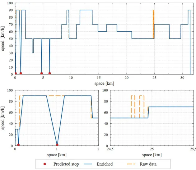
All the parameters in the [3.3] are functions of the selected driver type and of the traffic code. For further explanations on how they have been determined please refer to the chapter Calibration and Validation. The oscillation around constant speed segments constitutes the last space-based enrichment with respect to the previous version of the algorithm and an example of the final output is shown in fig.3.6:
3.3 – Speed Profile Prediction algorithm
Chapter 4
Calibration procedure
4.1
Methodology
This chapter represents an overview on how possible values for the parameters which mostly affect the prediction have been determined. The whole procedure is based on the acquisition of real data by an on-board recording across predefined scenarios. In particular, this section wants to provide a detailed description of the methodologies adopted during the measurements phase. Let it be clear that a rig-orous calibration requires an amount of time and resources that are beyond the availability of this thesis work. Nevertheless, the procedures described in this chap-ter have allowed to supply the algorithm with real-based foundations and can be considered an effective starting point for future works.
4.1.1
Scenarios
Two scenarios have been introduced so that the first could be used to tune the phases of acceleration and deceleration, while the second to evaluate the influence of the environment in terms of traffic, speed limits and stop events:
1. This scenario consists of an ad hoc maneuver where the driver performs a 0-50 km/h acceleration followed by a 50-0 km/h deceleration on a straight road. The range of speed has been assumed considering the use-case this algorithm has been developed for: the ZEZ is a urban contest where the most of the
maneuvers are included in this interval. Looking at fig4.1, it should be notice how the speed of 50 km/h is not achieved by the real driver: that is because of car OEMs are used to program cockpits where the displayed speed is slightly higher than the actual one.
Figure 4.1:1st scenario: 0-50-0 km/h acceleration and deceleration
2. In this case, a route across the city center of Bologna has been identified to be driven at different time-slots. This route in particular has been chosen for its peculiarity to present different speed limits and a high variation of traffic condition during the day. Thus, selecting adequate time-slots, the effects of every traffic code can be investigated.
4.1 – Methodology
Figure 4.2: 2nd scenario: from Via Umberto Terracini to Piazza Grigoris Lambrakis, Bologna
4.1.2
Measurements
The acquisition of the real speed profiles through the scenarios has been done by means of a GPS receiver (model: Navilock nl-8002u [19]) connected via USB to a laptop hosted in the passenger compartment. All the measures about vehicle speed and position are recorded with a 1 Hz sampling frequence and can be saved on PC thanks to the GNSS evaluation software developed by u-blox, named u-center. The Graphical User Interface (GUI) of the software offers the possibility for the users to select the variables of interest out of a long list and use them to feed real-time charts, like in fig. 4.4. Furthermore, data can also be grouped into tabs so that they can be easily copied into an Excel data sheet or into a Matlab workspace [fig. 4.5].
Figure 4.3: Measurement chain
Figure 4.4: u-center GUI: speed over time diagram view
4.1 – Methodology
4.1.3
Key Performance Indicators
In order to evaluate the overall goodness of predictions as well as the way they are affected by single parameters, key performance indicators (KPI) have been defined. Naturally, since the output generated by the algorithm is a speed profile prediction, an evaluation of the error in terms of speed had to be done, but always minding the energy management purpose. For this reason, two class of indicators have been introduced:
Speed KPI Energy KPI
The identification of speed KPI has been entrusted to a bibliography search in order to be aligned to the many in the past who have experimented the development of algorithms in this field [16][17][15]. This search revealed how the error in these kind of predictions are commonly evaluated by means of Mean absolute error (MAE) and BIAS, both expressed in km/h and defined as:
M AE = 1 n n X i=1 |Sp,i− Sr,i| (4.1) BIAS = 1 n n X i=1 Sp,i− Sr,i (4.2)
where Sp,i and Sr,i are respectively the predicted and the measured speed at point i and n is the total amount of point where the differences are calculated. MAE, not caring about the algebraic signs of the errors, expresses the mean distance between the prediction and real data. BIAS, instead, operates an algebraic sum so that self-compensation of the error can occur, resulting in possible low values of BIAS even in presence of high punctual errors. For this reason, BIAS on its own is not a reliable index to evaluate the goodness of the predictive model, but represents a powerful instrument to identify eventual issues related to a systematic under/overestimation of the speed.
Then, to define effective energetic indicators, [13] has been assumed as reference. In this document, SAE defines the parameters used to evaluate the goodness of tests
where a reference cycle must be followed by a human operator acting manually on pedals. First of all, three force components are calculated for both the predicted and the measured cycle:
Road load it represents the force required to win rolling resistance and drag force. It is expressed by the equation 4.3, where F0[N ], F1[ N
km/h], F2[ N (km/h)2]
are the cost down coefficients of the vehicle:
FRL = F0+ v · F1+ v2· F2 (4.3)
Positive inertial force it is associated only to positive values of acceleration (a+) and represents the force required by the vehicle mass to be accelerated. It is expressed by the equation 4.4, where M is the vehicle mass:
FI+ = M · a+ (4.4)
Negative inertial force it is associated only to negative values of acceleration (a−) and represents the force required by the vehicle mass to be decelerated:
FI− = M · a− (4.5)
Once the three forces have been defined, the relative energies can be retrieved by integrating the forces along the path length L, obtaining:
ERL = Z L 0 FRLdl (4.6) EI+ = Z L 0 FI+dl (4.7) EI− = Z L 0 FI−dl (4.8)
4.2 – Calibration
p and r are respectively referred to the predicted and measured (real) speed profile:
%ERL = ERLp− ERLr
ERLr · 100 (4.9) %EI+ = EI+ p − EIr+ EI+ r · 100 (4.10) %EI− = EI− p − EIr− EI− r · 100 (4.11)
While in case of an ICE vehicle differences in the negative inertial energy could be neglected, they have a huge impact in case of PHEV since they represent the amount of energy that can be potentially restored while braking. From this, the necessity for 4.11 to be introduced.
4.2
Calibration
After the acquisition of the real speed profiles, the data analysis could start. The target of the analysis was to tune the parameters related to acceleration, deceleration and traffic. It is important to consider that one series of these parameters needs to
Acceleration Kacc, τ Deceleration Kdec
Traffic CW, Ar, fr
Table 4.1: Calibration parameters
be determined for each driver type. Same approaches can be used for calibration in all the three cases, for example, by instructing the real driver on behaving differently during the measurements, or alternatively, recurring to three different real drivers properly recruited. In the next paragraphs, the procedures in case of driver type normal are shown for each parameter.
4.2.1
Acceleration and braking maneuvers
As anticipated in section 4.1.1, an ad hoc maneuver has been recorded as refer-ence for the calibration of acceleration and braking. The approach has consisted in a trial and error sequence where different combinations of Kacc, τ and Kdec have been tested, in order to make the profile generated by SPP matching with the measured one. The grade of matching has been evaluated on the base of MAE, starting from M AE = 6.37km/h to get to M AE = 2.42km/h [fig. 4.6].
Figure 4.6: Acceleration and braking: before(left) and after(right) calibration
4.2.2
Traffic: influence on average speed and oscillations
All the parameters related to traffic have been retrieved starting from measured speed profiles by way of frequence analysis. At first, portions of signal coming from different measured speed profiles, have been grouped by traffic code. Then, the Fast Fourier Transform (FFT) has been applied in Matlab to each signal obtaining the distribution of the amplitudes over frequencies. Since the SPP generates a space-based speed profile, also the frequencies must be expressed in terms of space (1/m) to be used in the algorithm. For this reason, a pre-processing is required by the measured signals before the FFT can be applied. In particular, a re-sampling of the signal have to be performed to make it sampled every meter instead of every second. At this point, applying the FFT, distance based frequencies and relative modules are obtained as shown by the example in fig.4.7. As expected, the amplitudes of these
4.2 – Calibration
Figure 4.7: Example of FFT applied to a distance-based measured signal
signals are characterized by a continue distribution over the frequencies, since infinite frequencies are required to perfectly approximate a non-periodic signal. Despite of it, to be represented in Matlab as couple of vectors, a signal must be discretized and this allow to easily identify frequencies with a high value of magnitude. The first consideration has been made looking at the amplitudes at f = 0: since they represent the average speed along the analyzed segments, they have been used to assign a CW value to every traffic code. Let’s assume:
the FFT be performed on J signals corresponding to J segments denoted by the same traffic code c;
lj be the length of the j-th segment;
A0,j be the magnitude at f = 0 of the j-th segment; The CW for the traffic code c has been retrieved as:
CWc= PJ j=1 A0,j Vlim,j · lj PJ j=1lj (4.12)
Consequently, once all the CW have been defined, a constant MAS can be assigned to each segment, as defined in the equation 3.1. After the MAS has been assigned, r cosines of magnitudes Ar and frequencies fr are added, as shown by the equation 3.3. This results in oscillation around the MAS value whenever it is reached by the driver. Here below, the procedure followed to retrieve Ar and fr as functions of the traffic code c is reported. Let’s assume:
the FFT be performed on J signals corresponding to J segments denoted by the same traffic code c;
four ranges of frequencies can be defined, denoted by r = 1,...,4;
Nj be the number of magnitudes An,r,j corresponding to the fn,r,j frequencies included in the range r, of the j-th signal;
Amplitudes Ar and frequencies fr for the traffic code c have been retrieved as:
Ar,c = PJ j=1( 1 Nj PNj n=1An,r,j) · lj PJ j=1lj (4.13) fr,c = PJ j=1( 1 Nj PNj n=1fn,r,j) · lj PJ j=1lj (4.14)
4.2 – Calibration
Chapter 5
Results and validation
Consequently to the calibration phase, the SPP has been applied to three dif-ferent scenarios to get a first evaluation of the performances at this progress of development. In the next sections, the results for each cycle will be shown as a com-parison between measured and predicted speed profile, expressed in terms of speed KPI and energy KPI.
5.1
Scenario 1
This cycle is the result of a 15.8 km route driven at 15.45 and governed by the three typical speed limit of a city center: 50 km/h, 30 km/h (residential areas), 70 km/h (ring road). Three traffic codes have been experimented (green, orange, black) whose lengths, in this particular case, have been well forecast by the MSP: the model, in fact, resulted to be perfectly centered (BIAS = −0.10 km/h) despite of the real driver more than once has exceeded the speed limit by a lot (m = 805 and m = 1243)[fig.5.1, 5.2].
Table 5.1: Scenario 1:speed KPI
KPI [km/h]
MAE 12.41
Table 5.2: Scenario 1:energy KPI Abs Rel [kWh] [%] ERL 0.005 -0.4 EI+ 0.032 -2.0 EI− 0.032 -2.0
5.2 – Scenario 2
Figure 5.2:Scenario 1: energy
5.2
Scenario 2
This scenario represents the one with the longest length (17831 m) and the most populated traffic codes vector (55 elements). Such a variety has been obtained doing the measurements at the rush hour (17.43). In this case, the predicted speed tends to be higher than the actual one, especially in the central area (from m 7000 to m 12000), but still keeping a narrow value of BIAS (3.31 −3.31 km/h)[fig.5.3]. Looking at the energy KPI, it is possible to see how this scenario is the only one where the inertial energies are overestimated[fig.5.4]. Possible reasons for this behavior will be discussed in detail in the next chapter, where possible solutions are introduced as future works.
Table 5.3: Scenario 2:speed KPI
KPI [km/h]
MAE 11.07
Table 5.4: Scenario 2:energy KPI Abs Rel [kWh] [%] ERL 0.004 3.55 EI+ 0.036 23.47 EI− 0.036 23.47
5.2 – Scenario 2
5.3
Scenario 3
This scenario has been introduced to test the robustness of the algorithm in case of a short length prediction (3,186 km). In this case it can be easily noticed how the oscillations of the predicted signal seems to have a totally different behavior with respect to the measured signal. This condition is largely due to the fact that, in this case, the traffic codes information has not been so reliable like in the other two previous cases. In general, has been observed how the predicted and the measured road load energy have the tendency to be coincident: this is in accordance with the low values of BIAS encountered and with the fact that all the three scenarios are denoted by a low value of average speed, resulting in small contributes of the term v2· F
2 [fig.5.5,5.6].
Table 5.5: Scenario 3:speed KPI
KPI [km/h]
MAE 8.27
BIAS 1.88
Table 5.6: Scenario 2:energy KPI
Abs Rel
[kWh] [%]
ERL 0.003 1.76 EI+ 0.046 -9.82
5.3 – Scenario 3
Figure 5.5: Scenario 3: speed
Chapter 6
Conclusions and future works
6.1
Initial and final speed
Looking at the energy KPI in Scenario 1 [fig.5.2] and Scenario 2 [fig.5.4], it can be noticed that both of them present coincident errors for positive and negative inertia (%EI+ = %EI−). On the contrary, this condition is not found in Scenario
3 [fig.5.6]. This behavior is coherent with the way inertial forces are defined: they represent the energy requested by the vehicle to be accelerated and decelerated, including the work done by non-conservative forces. Consequently, the cumulative overall inertial energy, for a cycle whose initial and final speed are coincident, is equal to zero. So, the coincident errors in first two cases are due to the fact that both the predicted and the measured initial and final speeds are equal to zero. Instead,in Scenario 3, both the predicted and the measured final speeds are equal to zero, while the initial speeds are not coincident. This observation could appear as trivial, but it highlights how the prediction accuracy can be increased when initial and final speed are well-imposed. Since in the current version of the algorithm these values are imposed manually, a possible improvement could be the implementation of a further algorithm branch that generates them by basing on navigation data in the vicinity of ZEZ-in and ZEZ-out gates.
6.2
Oscillation energy
The comparison of the energy KPI brings to an additional observation: the nar-row underestimation of the inertial energies in Scenario 1 (≈ −2%) and 3(≈ −10%) are quite in contrast with the overestimation that took place in Scenario 2 (> +20%). A possible cause for this behavior has been investigated in the oscillations introduced to reproduce the effects of the traffic flows, since their reliability is still to be veri-fied. In fact, despite of magnitudes and frequencies of these oscillations have been retrieved starting from the frequency analysis of real data, as done by many before, the procedure described in chapter 5 is an empirical approach that can not count on bibliographic references. Thus, to make a first evaluation of this methodology, predictions for all the three scenarios described in chapter 5 have been executed before and after the oscillation were added to the MAS. The results of this series of comparative simulations are reported in fig.6.1. As can be easily seen, MAS, BIAS
Figure 6.1: Effects of oscillations on KPI
and road load energy are quite unaffected by the introduction of the oscillations. The situation is totally different for the inertial energies: underestimation in Scenario 1 e 3 is effectively reduced by the introduction of the oscillations, while is way too over-compensated in Scenario 2. Unfortunately, the current information availability on traffic codes and measured cycles is not sufficient for an accurate identification of the causes for this misalignment. Nevertheless, one general conclusion can be retrieved: in three out of three cases the inertial energies would be heavily underestimated without the addition of the oscillations. This trend confirms how the oscillation con-stitute an essential part for a robust prediction and how this topic deserves to be