Job Instability and Fertility: How do “precarious" workers deal with childbearing? Italy and EU countries case studies

(1)

UNIVERSIT `

A POLITECNICA DELLE MARCHE

Dottorato di Ricerca in Economia Politica

XV Ciclo Nuova Serie

Tesi di dottorato

Job Instability and Fertility:

How do ‘precarious’ workers deal

with childbearing?

Italy and EU countries case studies

Isabella Giorgetti

Supervisore

Prof. Stefano Staffolani

Correlatore

Prof. Matteo Picchio

Coordinatore

Prof. Riccardo Lucchetti

(2)

(3)

Acknowledgments

A special thank goes to Prof. Stefano Staffolani and Prof. Matteo Picchio for their excellent research assistance and support in developing the present project. Interacting with them has been incredibly productive and challeng-ing since the first day of my Ph.D. studies.

I wish to express my best gratitude to Claudia Pigini, not only for her excellent research assistance, but also for her supportive behavior throughout the whole Ph.D. programme.

I would like to thank Prof. Massimilaino Bratti and Prof. Daniela Vuri for useful comments, revisions, and suggestions.

I acknowledge Eurostat for providing the dataset EU-SILC (European Statistics on Income and Living Condition). Any errors are the authors’ sole responsibility.

(4)

(5)

Abstract

Chapter I

Fertility patterns have changed significantly since the 1960s in most advanced Western countries, with trends towards later childbearing, smaller families and an increase in childlessness. Described as ‘one of the most remarkable changes in social behaviour in the twentieth century’ (Leete 1998), declining fertility is one aspect of a range of demographic changes interpreted in the literature as the outcome of various socio-economical changes occurring as a result of modernisation. This process, the timing of which is variable across countries, is called the Second Demographic Transition (van de Kaa 1987; Lesthaeghe 1995). Since the mid-1980s,the macro level association between female labour force participation (FLFP) and Total Fertility Rate (TFR) has become positive (Ahn and Mira 2002; Engelhardt and Prskawetz 2004; Billari and Kolher 2004). This review starts with an overview of theories on the economics of fertility and the empirical implications in developed countries, seeking to explain fertility decline more generally and, finally, focusing on the relationship between job instability in the labour market and fertility choices.

Chapter II

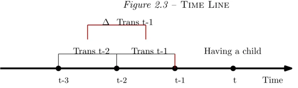
This empirical study aims to investigate the relationship between the low female participation rate in the labour market and the “lowest-low” fertil-ity rate in Italy during the recent econimc downturn (started from 2008), focusing on the effects of the implementation of the new types of flexible forms of contracts have had on the young couples’ fertility choice, after the reform known as “Biagi Law” (L. 30/2003) in Italian labour market. Using Italian’s individual data from longitudinal EU-SILC dataset (2004-2013), I consider all women between 15 and 45 years old, living with the partner, and who are active in the labour market. I build the job (in)stability measure for both the partners by their transitions in the activity statuses into the labour market during the two previous years. I estimate a First Difference Linear Probability Model (accounting for the unobserved heterogeneity and potential presence of endogeneity) in order to investigate the short-run effect

(6)

main findings show that, for women, remaining in temporary contracts affects negatively, and furthermore this occupational status discourages childbearing more than being in unemployment because of higher opportunity-costs. For men, instead, finding a job boosts the choice of having at least an another child, while the fall and the remaining in unemployment depress the fertility.

Chapter III

The trends of decline in TFR varied widely across countries. In Northern European countries, the decline started early but has oscillated around 1.85 children per women since the mid-1970s. By contrast, among Eastern and Southern European countries the decline has been slower, starting in the mid-1970s, but reached an extremely low level of 1.3 in 1994 before slowly starting to edge up. The latters are known as ‘lowest-low-fertility’ countries because they have total fertility rates persistently around 1.3 children per woman (Kohler et al. 2002). Exploiting individual data from the longitudi-nal EU-SILC dataset from 2005 to 2013, the present study investigates the cross-country short-run effect of job instability on the couple’s choice of hav-ing an addictional child. I build job instability measure for both the partners by the lag of economic activity status had in labour market (that encompasses holding temporary or permanent contract, or being unemployed). In order to account for the unobserved heterogeneity and potential presence of endogene-ity, I estimate a Two Stage Least Square Model (2SLS) in first differences and under sequential moment restriction. Then, grouping European coun-tries into the six different welfare regimes, I can estimate the heterogenious effects of instability in the labour market on childbearing among different institutional settings of European welfare. The principal result is that the cross-country average effect of job instability on couple’s fertility decisions is not statistical relevant because of the huge country-specific fixed effects, even if having a temporary job for women encourages chilbearing, in average. When I analyse these impacts distinguishing also through welfare regimes’ classification, the institutional structure and linked social active policies re-veal a varying family behaviour for fertility choices. In low-fertility countries, however, it is confirmed that the impact of parents’successful labour market integration might be ambiguous, due to the absence of child care options.

(7)

Abstract

Capitolo I

Gli scenari di fertilità sono cambiati in modo significativo dal 1960 nella maggior parte dei paesi occidentali avanzati; essi seguono trend che eviden-ziano effetti di posticipazione nelle scelte di fertilità, si hanno famiglie di più piccole dimensioni e aumentano nel numero quelle senza figli. Ad oggi, il calo della fertilità è descritto come ‘uno dei più gravi cambiamenti nel comportamento sociale del XXI secolo’ (Leete 1998) e si presenta come uno degli aspetti di una serie di cambiamenti demografici e di profonde trasfor-mazioni socio-economiche. Questo processo, che si presenta con una diversa tempistica tra i vari paesi, è conosciuto in letteratura come la Seconda Tran-sizione Demografica (van de Kaa 1987; Lesthaeghe 1995). Dalla metà degli anni 1980, la correlazione a livello macro tra la partecipazione femminile alla forza lavoro (FLFP) e il Tasso di Fecondità Totale (TFR) ha cambiato segno, diventando positivo (Ahn e Mira 2002; Engelhardt e Prskawetz 2004; Billari e Kolher 2004). Questa review inizia con una panoramica delle teorie sull’economia della fertilità e delle implicazioni empiriche evidenziate per i paesi sviluppati. In questo lavoro si cerca di spiegare il declino della fertilità, in generale per poi concentrarsi sulla relazione che esiste tra l’instabilità nel mercato del lavoro e le scelte di fertilità.

Capitolo II

Questo lavoro si propone di indagare il rapporto tra il basso tasso di parteci-pazione femminile al mercato del lavoro e l’ancora più ridotto tasso di fecon-dità in Italia durante gli anni della recente crisi economica (iniziata a partire dal 2008), con un focus sugli effetti generati dai nuovi tipi di contratti a forme flessibili introdotti con l’attuazione della legge ‘Biagi’ (L. 30/2003) sulle gio-vani coppie circa le loro scelte di fecondità. Dai dati individuali longitudinali italiani raccolti dal dataset EU-SILC (2004-2013) estraggo un campione di tutte le donne tra i 15 e i 45 anni conviventi con il partner e che sono attive nel mercato del lavoro. Costruisco la misura di instabilità del lavoro, per entrambi i partner, attraverso le loro transizioni occupazionali avvenute nel mercato del lavoro e registrate nei due anni precedenti e stimo un modello

(8)

di breve periodo che l’instabilità del lavoro genera nella scelta da parte delle coppie di avere un (altro) figlio. I principali risultati mostrano che, per le donne, mantenere un contratto a tempo determinato influisce negativamente e l’effetto è statisticamente significativo sulla scelta di procreazione. Questo produce un effetto maggiore anche rispetto a quello generato dal restare in disoccupazione. Per gli uomini, invece, è il trovare un lavoro la determinante che aumenta la probabilità della scelta di fecondità, mentre la caduta e il restare in disoccupazione sono effetti che la deprimono.

Capitolo III

Il declino del tasso di fecondità totale (TFR) ha subito negli anni ampie vari-azioni nella misura e differisce tra i paesi europei. Nei paesi del Nord Europa, il trend negativo è iniziato presto, ma si è fermato e oscilla intorno al 1,85 figli a partire dalla metà degli anni 1970. Al contrario, tra i paesi dell’Europa orientale e meridionale il calo è stato più lento, è partito dalla metà degli anni 1970, ha raggiunto un livello estremamente basso pari al 1,3 nel 1994, per poi iniziare lentamente a riprendersi. Questi paesi sono conosciuti come i paesi con più bassa fertilità proprio perché hanno tassi di fecondità che oscillano intorno a 1,3 figli per donna (Kohler et al. 2002). Utilizzando i dati individuali dell’indagine europea del reddito e sulle condizioni di vita (EU-SILC) 2005-2013, il presente studio indaga l’effetto cross-country e di breve periodo che l’instabilità del lavoro ha sulla scelta della coppia di avere un figlio in più. Costruisco la misura dell’instabilità per entrambi i partner dal ritardo del proprio status di attività (che comprende il contratto tem-poraneo, permanente, o l’essere disoccupato), concentrandomi in particolare sulle scelte di fecondità delle coppie attive nel mercato del lavoro. Al fine di tenere conto della eterogeneità non osservata e della potenziale presenza di endogeneità, stimo un modello Two Stage Least Square (2SLS) in differenze prime assumendo la condizione di esogeneità sequenziale. Poi raggruppo i paesi europei sfruttando una classificazione di sei regimi di welfare differenti e stimo gli effetti eterogenei dell’instabilità nel mercato del lavoro sulle scelte di fecondità che si manifestano tra i diversi contesti istituzionali. Il risultato principale di questo lavoro è che l’effetto medio cross-country che l’instabilità nel mercato del lavoro genera sulle decisioni di avere bambini prese da parte delle coppie non è statisticamente significativo, a causa degli enormi effetti fissi specifici per paese. Solo la presenza di lavoro temporaneo per la donna promuove in media le scelte di fecondità. Inoltre, quando distinguo tra i diversi regimi di welfare, i risultati rilevano invece una variazione di compor-tamento profonda tra le coppie in tema di maternità, la quale è molto legata alla struttura istituzionale e alle politiche sociali attive promosse dai propri

(9)

(10)

(11)

List of Figures

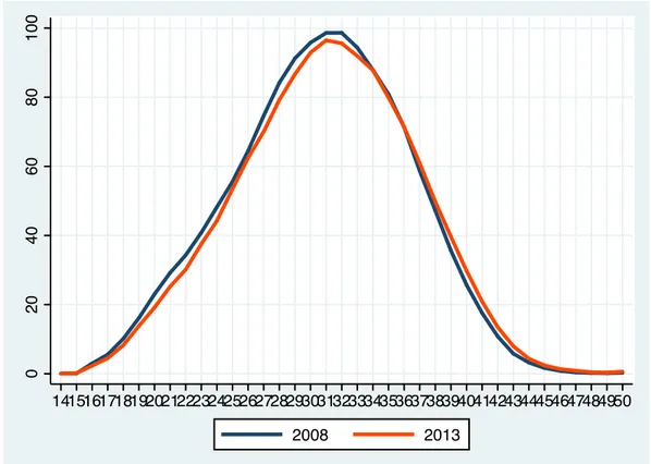
Figure 1.1: Interaction of the demand for quality and quantity of children . . . 8 Figure 1.2: Time allocation and fertility decisions . . . . 12 Figure 1.3: Effect of an increase in the female wage . . 14 Figure 1.4: _{effect of an increase in the husband’s income 16} Figure 2.1: Italian age-specific fertility rate - 2008 vs

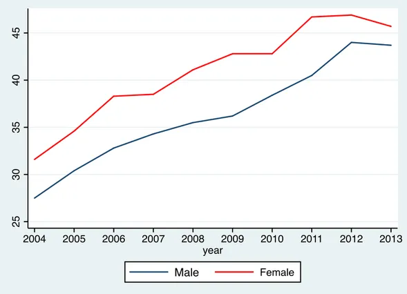
2014 (Values per 1,000 women) . . . 41 Figure 2.2: Percentage of temporary employees on

to-tal by gender (15-24 aged people, years 2004-2013) . . . 43 Figure 2.3: Time Line . . . 52 Figure 3.1: Gender gap in employment rates, EU

coun-tries, 2008-2013 . . . 83 Figure 3.2: _{Female temporary employees on total}

em-ployment, EU countries, 2008-2013 . . . 84 Figure 3.3: Time Line . . . 96 Figure 3.4: Total Fertility Rate, 2013 - EU countries . . 113 Figure 3.5: Qualifying period for unemployment

bene-fits - EU countries . . . 114 Figure 3.6: Number of children across EU countries . . . 116

List of Tables

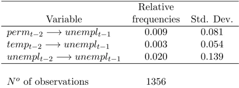
Table 2.1 Transitions in economic activity status . . . 46 Table 2.2 Summary statistics . . . 47

(14)

levels and first differences

Table 2.4 Estimation results of the model for fertil-ity controlling for heterogeneous effects in first differences . . . 61 Table 2.5 Robusteness checks - First Differences Linear

Probability Models . . . 66 Table 2.6 Number of child(ren) by woman age cohorts

-Percentage values . . . 72 Table 2.7 Transitions in economic activity status . . . 73 Table 3.1 Sample’s composition by Country and Welfare

Regimes . . . 89 Table 3.2 Economic activity status . . . 90 Table 3.3 Summary statistics . . . 91 Table 3.4 Estimation results of the model for fertility in

levels and first differences . . . 99 Table 3.5 Estimation results of the model for fertility

con-trolling for welfare regimes’ heterogenious ef-fects in first differences . . . 105 Table 3.6 Number of child(ren) by woman age cohorts

(15)

Introduction

Since the 1990s, economic uncertainty has been becoming an essential fac-tor in explanations of the decline in fertility and the postponement planning of family formation across Europe, particularly when the aim is concerned to explain the developments recorded in Southern and post-socialist Central and Eastern Europe (e.g. Kohler and Kohler 2002). The start of the eco-nomic recession in 2008 has triggered renewed interest in the role of ecoeco-nomic uncertainty for family dynamics. In view of the consequent financial and eco-nomic volatility across Europe, the relationship between ecoeco-nomic household conditions and family dynamics enlarges its notoriety and becomes a major topic of public interest.

Economic uncertainty may be perceived as an individual risk factor, linked to phases in the life course that are characterized by unemployment, part-time work, working on a term-limited contract, or difficulties entering and reentering the labour market (e.g., Mills and Blossfeld 2005).

It may also be understood as an aggregate phenomenon that reflect gen-eral uncertainties felt by all people during, for instance, an economic recession (Sobotka et al. 2011). Most recently, empirical research has stressed the idea of economic uncertainty as a potential root of the fertility declines observed across Europe since the 1980s.

The evidence of correlations in some countries between low fertility rate and adverse economic conditions has boosted this interest. First, South-ern Europe countries recorded extreme fall in annual birth rates during the 1990s owing to segmentation of Southern Europe’s labour markets, deter-mining high levels of youth unemployment and precarious patterns of entry into the labour market (McDonald 2000). Second, in Central and Eastern Europe, birth rates declined quickly after the abolishment of the communist regimes. The growth of uncertainties in labour markets during the transition from planned to market economies has negatively affected fertility in these countries. (Ranjan 1999). Furthermore, deregulation, internationalization, and globalization in the labour market have determed an increase in economic uncertainty, especially for young adults that face them into the partnership

(16)

ity in employment are now evaluated as the main driving forces behind the postponement of childbearing in contemporary Europe.

While the first decade of the new millennium documented a moderate increase in fertility rates across Europe countries, their policy makers still consider their current fertility levels as too low and this situation is becoming worrying after the beginning of the financial crisis and economic volatility in Europe in 2008 has emphasized this issue (Sobotka et al. 2011).

My thesis try to insert in this brach of literature and addresses this recent research topic, focusing on the effect of job instability on fertility. This is an issue on which evidence is still scarce and the major reason is linked to the fact that identifying the casual effect of job instability on fertility must be account for endogeneity problems (see paragraph 1.4 for more information). It is composed by three chapters. In the first one I introduce an overview of theories on the economics of fertility and the empirical implications when they take place in fertility behaviour in developed countries, seeking to ex-plain fertility decline more generally and, finally, focusing on the relationship between job instability in the labour market and fertility choices.

In the second one, I investigate the relationship between the low female participation rate in the labour market and the ‘lowest-low’ fertility rate in Italy during the recent econimc downturn (started from 2008), focusing on the effects of job instability measures for both the partners biult by their occupation transitions have on chilbearing. Using Italian individual data from the longitudinal European Survey of Income and Living Conditions (EU-SILC) from 2004 to 2013, I estimate a First Difference Linear Probability Model (accounting for the unobserved heterogeneity and potential presence of endogeneity) in order to investigate the short-run effect of job instability of both the partners on the couples’ choice of having at least an another child, controlling for the other socio-economic characteristics.

In the third one, I enlarge my focus of the study at 21 European countries to capture the cross-country average effects and also the heterogeneous effects of instability in the labour market on childbearing across the different Eu-ropean welfare regimes in order to better understand the real detarminants of fertility choices introducing institutions’ role. Finally, the work ends with explanations of final remarks.

(17)

Chapter 1 Literature review

1.1 Introduction

Since the 1960s in most developed Western countries, fertility trends have changed significantly, with paces towards later childbearing, smaller families and an increase in childlessness. Described as ‘one of the most remarkable changes in social behaviour in the twentieth century’ (Leete 1998), fall in fertility is one aspect of a range of demographic and socio-economic trans-formations occurring as a result of modernisation. This trend, the timing of which varies across countries, is called the Second Demographic Transition (van de Kaa 1987; Lesthaeghe 1995): in fact, the decline of fertility below replacement level1 was previously viewed as the most important feature of the transition in the demographic literature (van de Kaa 1987).

Fertility decline is mainly due to fertility postponement behaviour of households.2 _{This one raises several issues concerning demographic ageing}

and its socio-economic implications (for example for social security provi-sion), the possible future decrease in labour supply and its impact on future economic growth, and the prospect of total population decline.3

Since the mid-1980s,the macro level association between female labour force participation (FLFP) and Total Fertility Rate (TFR) has become posi-tive (Ahn and Mira 2002; Engelhardt and Prskawetz 2004; Billari and Kolher

1_{The replacement level of fertility is the level at which the population of a society,}

net of migration, would remain stable. In contemporary societies this occurs with a total fertility rate of around 2.1. The total fertility rate is a measure that expresses the mean number of children that would be born to a woman if current patterns of fertility persisted throughout her childbearing life.

2_{Some authors suggest rather that delayed childbearing constitutes a ‘postponement}

transition’ towards a late-fertility regime (see Kohler, Billari and Ortega 2002).

3_{Increasing concern about the possible consequences of fertility decline is evident in}

(18)

2004). But a meta-analysis of micro level studies (Matysiak and Vignoli 2008) indicates that the association between FLFP and fertility remains negative, but its magnitude is stronger where the male-breadwinner model prevails (e.g. Southern Europe), and weaker in the Nordic Countries where more generous and/or efficient protection systems have been implemented to rec-oncile motherhood with work (Esping-Andersen 1999; Adser`a 2004; Del Boca and Sauer 2009). During the 1990s, the increasing competition in the labour markets and employers’ rising demands for workers flexibility have further affected childbearing in general (Mills and Blossfeld 2005). The employment instability with precarious jobs increases economic uncertainty and becomes more intense the difficulties among the young in their transition to adulthood, when they start their labour market careers, try to improve their economic position and begin to plan family project (e.g. McDonald 2006 and Vignoli, Drefahl and De Santis 2012).

This review starts with an overview of theories on the economics of fertil-ity and the empirical implications when they take place in fertilfertil-ity behaviour in developed countries, seeking to explain fertility decline more generally and, finally, focusing on the relationship between job instability in the labour mar-ket and fertility choices.

In the next section I seek to review the choice-theoretic static framework of neoclassical economics originated in the pioneering paper by Becker (1960) known as ‘New Home Economics’ in which the theory of the consumer is ap-plyed to explain the choice of complited family size with regard to variations in family income and the “prices”, or opportunity cost of children.

In the third section, I review the literature on dynamic models of fertil-ity behaviour over the parents’ life cycle. I outline the ways in which these models linked to the static models and examine what implications they pro-vide for dimensions of fertility behavior which cannot be addressed with the earlier models, namely, the timing of first births, spacing of children, and contraceptive behavior.

After this review of the theoretical models of fertility, I discuss, in section 1.4, the broad issues in estimating the implications of the theory for observed fertility behavior: the fundamental identification problems which arise in as-sessing the impact of prices and income on both lifetime and lifecycle fertility behavior.

So, I introduce the Easterlin’ hypotesis to have a comprehension of macroe-conomic approach model on fertility behaviour and to have an alternative framework to better understand the recent branch of literature that focus-ing on the studies that analyse the statistical association between the “job instability” and the fertility choices, that I present at the last section.

(19)

Static

1.2 Static models of fertility: “New Home Economics”

The microeconomic approach to explaining fertility behavior is an application of neoclassical models of consumer demand: parents as rational consumers choose the quantity (or better, the number) of children which maximizes their utility subject to the price of children and the budget constraint they face. Such models are “static” because they assume that the unit of time for these choices is the parents’ lifetime perspective as one period.4

More formally, they assume that parents maximize an utility function,

U = U (n, s) (1.1)

which depends on the outcome of interest, the number of children, which is denoted by n, and a good, s, which characterizes all other consumption and the utility function has all the conventional properties, i.e., increasing and concave in both arguments. In this simple setting, parents are assumed to choose n and s so as to maximize Equation (1.1) subject to the following (conventional) budget constraint:

I = πss + pnn (1.2)

where I is the household’s income, pn is the ”price” of children per unit,

and πs is the price of the composite commodity per unit. Taking the price

of the composite good as numeraire, this simple model yields a standard demand for children function as following:

n = N (pn, I) (1.3)

which depends upon the price of children and parental income. The effect of changes in the price of children on completed fertility size are characterized by the income and substitution effects of consumer theory and variations in

4_{They ignore such issues as the possibility that the constraints that parents face, in}

terms of prices and budget constraints, may vary over the parents’ life cycle, the potential uncertainty that parents may have at any point in time about these constraints in future periods, or the apparent fact that fertility outcomes unfold over time as well. These possibilities and their implications will be considered in the dynamic models of fertility behavior below.

(20)

parental income rise the income effects with respect to the “purchase” of children.

The first empirical challenge is to find proxies for the price of children: in fact, given a parametric specification of Equation (1.3)5 and assuming that children are not Giffen goods, one can estimate the price responsiveness of the demand for children due to exogenous variations in the cost of rearing children or changes in governmental policies which affect the cost of children (e.g., changes in tax deductions for dependents or public assistance benefits). The second one is concerned on determining the direction and magnitudes of the effect of income on the demand for children, although there has been a presumption in the literature that they are positive, i.e., children are not inferior goods. Finally, the challenge of adapting neoclassical economic mod-els to fertility behavior has driven a number of important extensions of this simple model, addressing the distinctive aspects of this set of behavior, and, also, representing important adaptations of the application of economics to human behavior (Hotz et al. 1997).

In the following sections, I examine two important contributions to the early literature on the economics of fertility so called “New Home Economics” or “Chicago School” that started in the 60s. In the first one, the quality-quantity model of fertility in which parents demand numbers of children with certain qualities. The second one is concerned with the importance of alloca-tion parental time, especially for the mothers those mainly nurture children. Elements of these two model features are shown by Becker (1960) and Min-cer (1963). Then they are synthesized by Willis (1973), with some further implications of the quality-quantity model developed in Becker and Lewis (1973).6, and they are recalled by Becker (1991) into the book “A Treatise of the Family”.7

1.2.1 The quality-quantity model

With regard to the observations that fertility tends to be negatively related to income both in time series and cross section, Becker (1960) rejected as-sertation that children are inferior goods or that high income families, who spend more on their children, have lower fertility because they face higher prices of children. Instead, he argued that the puzzle could be inserted within

5_{See Browning (1992) for a literature overview of some methods of defining children}

variables to yield a demand function.

6_{Willis (1987) suggests that these papers mark the emergence of the economics of the}

family as a distinct subfield in economics.

(21)

The quality-quantity model

a model of stable preferences in which children are a normal good8 _in

addi-tion to the quantitative dimension represented by the number of children and a qualitative dimension associated with the choice of expenditures per child. He assumed a simple model of fertility behavior in which parents had preferences both for the number of children and the quality per child. This static lifetime model is an adaptation of the simple model is shown above. In particular, a new married couple acts as a unitary household with a single decision maker with preferences given by the utility function

U = U (n, q, Z) (1.4)

where n continues to denote the number of children, Z the parents’ stan-dard of living, and q is the quality per child. In place of Equation (1.2), the household’s lifetime budget is now as

I = πcnq + πZZ (1.5)

where I continues to be the total family lifetime income, πc is a price

index of goods and services for children and πZ is a price index of goods and

services for adults. The particular feature of this problem is that the budget constraint is nonlinear because quantity and quality enter multiplicatively. It is this quality-quantity interaction that leads to certain distinction features of the demand for children. In the model of Equations (1.4) and (1.5) Becker (1960) adds an implication such as the income elasticities of demand for n, q and Z must satisfy the following relationship

α(εn+ εq) + (1 − α)εZ = 1 (1.6)

where α is the share of family income for children and the ε indicate income elasticities. If children are normal goods and total expenditures on children are an increasing function of income, then the sum of the income elasticities of the number and quality of children must be positive (i.e., εn+

εq > 0). But it is still possible that the income elasticity of demand for the

number of children is negative (i.e., εn< 0) if the income elasticity of quality

8_{In “A Treatise on the Family” (Becker 1991) it becomes also durable good and without}

(22)

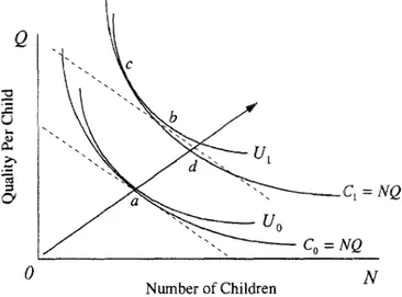
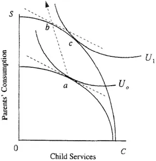
Figure 1.1 – Interaction of the demand for quality and quantity of children

Source: V.J. Hotz, J.A. Klerman and R.J. Willis (1997), p.296, Fig.7

is high enough.9 _{He ended up arguing that income is likely to have a small}

positive effect on fertility, but believed that a negative correlation between birth control knowledge and income might change the overall sign of the income-fertility relationship to negative. Willis (1973) and Becker and Lewis (1973) provide a formal analysis of the quality-quantity model in which the implications of the nonlinearity in the budget constraint in Equatione (1.5) are explored.

Maximizing household utility in Equation (1.4) subject to the family bud-get constraint in Equation (1.5) yields the following first-order conditions:

M Un= λqπc = λpn; M Uq = λnπc= λpq (1.7)

where the MU ’s are marginal utilities and the p’s are marginal costs or shadow prices of the number of children and quality per child, respectively, and λ is the marginal utility of income. These conditions imply that the shadow price of the number of children is an increasing function of child quality, while the shadow price of child quality is an increasing function

9_{Although Becker was unable to cite estimates of the demand for other goods in which}

the income elasticity of demand for quantity was negative, he cited studies showing that quality elasticities tended to be larger than quantity elasticities.

(23)

The quality-quantity model

of the number of children. Furthermore, since n and q are chosen by the household, the shadow prices are endogenous.

The household’s optimal choice of number and quality of children is shown in Fig.1.1. Equilibrium is at point a where the indifference curve U0 is

tan-gent to the budget constraint, co = nq = (I − πZZ(πc, πZ, I))/πc, where

c0 is the household’s real expenditure on children and Z(πc, πZ, I) is the

de-mand function for parents’ standard of living. The indifference curve must be more concave than the budget constraint, c0 = nq, which is a rectangular

hyperbola.10

The nonlinearity of this budget constraint causes a quality-quantity in-teraction as income increases that yields a substitution effect against the number of children and in favor of quality per child (if the income elasticity of demand for quality exceeds the income elasticity of demand for number of children). In fact, in Equation (1.6) the marginal rate of substitution be-tween the quantity and quality of children is M Un/M Uq = pn/pq = q/n so

that the relative cost of the number of children increases if the ratio of quality on quantity rises (εn > εq). If the income elasticities for quality and quantity

were equal, the income-expansion path would be given by ray Oad and the ratio of quality to quantity and the marginal rate of substitution between quality and quantity both remain constant. If εn > εq, the total effect of an

increase in income that raises total expenditures on children from c0 to c1

is to move optimal consumption from point a to point c. This total effect may be disaggregated into a “pure income effect”, holding pn/pq constant

from point a to point b, and an “induced substitution effect” from point b to point c. As drawn in Fig.1.1, the total effect of an increase in income do not change the number of children because the pure income effect, which tends to increase desired fertility, is crowded out by a substitution effect that yields an increased expense per child associated with higher desired quality.

Becker and Lewis (1973) incorporate in the budget constraint of Equatin (1.6) the costs of the number of children (independent on quality) and costs of quality (independent on the number of children), as follow

I = πnn + πqq + πcnq + πZZ (1.8)

where πnand πq, represent these independent cost components so that the

marginal costs of numbers and quality become, respectively, pn= πn+πcq and

pn= πn+ πcn. They consider a case (as an application) in which πq = 0 and

10_{So, quality and quantity cannot be too closely substitutable in consumer preferences}

(24)

πn represents the opportunity cost of fertility control, such as introduction

of a new contraceptive method such as the oral contraceptive pill will reduce the cost of averting births and, therefore, increase the marginal cost of a birth without affecting the marginal cost of child quality. The increase in pn,

leads to a substitution effect against fertility which increases q/n, thereby inducing a further substitution effect against fertility and in favor of quality. Their analysis suggests that the elasticity of demand for number of chil-dren is likely to be more negative with respect to variables such as contracep-tion or maternity costs, which affect πn, than it is with respect to variables

such as the female wage which affect πc. A parallel analysis suggests that

a decrease in πq due t, an increase in parents’ education, may have a

nega-tive effect on fertility because the direct substitution effect which increases q causes an increase in pn. Other examples of factors affecting πq might include

the quality of a neighborhood, school quality, and cultural factors.

There are several alternative concepts of child quality in the literature.11

Becker (1991) considers children are as a durable consumption good and child quality is indexed by expenditures per child in much the same way that quality might be estimate by price in markets for cars in a world of perfect-informed consumers. The dominant view of child quality in the lit-erature on fertility behavior and family economics is based on the theory of human capital form, in which parents parents, who care about the lifetime economic well-being of their children, influence their children’s well-being ei-ther through the direct transfer of money or by investing in the child’s human capital.

1.2.2 Parental time allocation

The second major reason for explaining the presence of a negative relationship between income and fertility, in addition to quality-quantity interaction, is

11_{The concept of “child quality” synthesizes different factors of children’s well-being,}

such as time, effort, and money for their care and growing up, their likelihood of not dropping out of school, and the level of parents’ subjective well-being which in turn has relevant effects on children’s psychological development. Willis (1973), for example, defines child quality as a function of the resources parents devote to each child. See Browning (1992) for a survey of this literature: a number of indirect approaches have been suggested to estimate the “cost of children” based upon equivalency scales which depend upon how observed household consumption patterns, e.g. proportion of income spent on food, vary as income and household consumption vary. But, as Hotz et al. (1997, p. 298) state: “this literature is not helpful in understanding fertility behavior because (a) estimates of child costs are derived under the assumption that variations in household composition, including the number of children, are exogenous and (b) total expenditures on children are not decomposed into an endogenous part reflecting child quality and an exogenous part measuring the price index of children faced by the household.”

(25)

Parental time allocation

the hypothesis in which the association of higher income and a higher cost of female time is due to increased female wage rates raising the value of female time in nonmarket activities. The assumption is that childrearing is a relatively time intensive activity, especially for mothers, so the opportunity cost of children increases for the above reasons, the substitution effect against children rises.12

Willis (1973) introduces a simple static, lifetime framework for analyzing the interplay between time allocation, labour supply and fertility behavior in which all the choices are assumed to be made at the beginning of marriage and are not subject to revision: In fact, he assumes that the married couple is the decision-makers who derive utility from adult standard of living and from the number and quality of children as given by the utility function in Equation (1.4).

Following Becker (1965), the household uses the nonmarket time of house-hold members and purchased goods as inputs into househouse-hold production pro-cesses whose outputs enter into the utility function. First assumption is that only the wife participates in the production of household commodities while the husband is fully specialized in market work and his income, H, is exoge-nous. Total family income is I = H + wL where w is the wife’s real wage and L is her labour supply. Second one is that satisfaction from children is measured by “child services”, c = nq, and the determination of the division of c between the number and quality of children is not considered for the moment. Third one is that household production has constant returns of production functions, s = g(ts, xs) and c = f (tc, xc), where ts and tc are the

wife’s time inputs xs and xs are purchased goods devoted, respectively, to

the production of adult standard of living and child services. Finally, the key assumption of the model is that the production technology for children is time intensive relative to the technology for parents’ standard of living. The total time of the wife, T, is allocated between home and work that is T = tc+ts+L. Purchases of market goods are constrained by total household

income so that I = H + wL = xc+ xs .

The equilibrium of this model is shown in Panel A with an Edgeworth Box diagram (Fig.1.2): the horizontal dimension of the box measures the total amount of wife’s time that is devoted to household production (i.e. tc+ ts = T − L) and the vertical dimension measures the total expenditure

on goods (i.e. xc+ xs = T + wL). When the wife does not work, the diagonal

corners of the Edgeworth box are OO’, if the wife works, the northeast corner

12_{The cost of time hypothesis was first advanced by Mincer (1963) and then it is}

devel-oped by Becker’s (1965) household production model. This relationship between fertility and female labour supply has become a standard feature of models of household behavior.

(26)

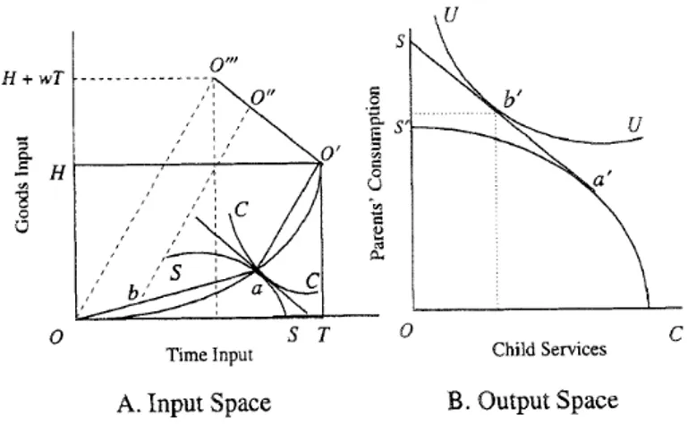
Figure 1.2 – Time allocation and fertility decisions

of the box moves to points such as O” or O”’ where the slope of the line O’O”’ is determined by the wife’s market wage w.

Assuming that the wife does not market work, all possible efficient allo-cations of time and goods occur along the contract curve, OO’. Within the box, isoquants corresponding to increasing outputs of child services (CC ) come from the origin at O while isoquants for parents standard of living (SS ) originate at O’. Because of the assumption that children are relatively time intensive, it implies that the contract curve lies below the diagonal of the box. The common slope at the tangency in absolute value between CC and SS at point a is equal to the shadow price of the wife’s time ω, given by the ratio of the marginal products of time and goods in each activity, and it is equal to the value to wife’s market wage given by the slope of OO”’. The corresponding outputs of c and s are indicated at point a’ on the production possibility frontier in Panel B (Fig.1.2). If the output of child services is increased by moving along the contract curve to the northeast of point a in Panel A, the shadow price of time increases because ratio of goods on time in the production of both c and s increase; so, given that children are relatively time intensive, an increase in the price of the time input leads to an increase in the relative cost of the time intensive output. Thus, the relative shadow price of children, πc/πs, which is equal to the (absolute value of the) slope of

the production possibility frontier in Panel B, tends to increase as the output of children rises above the level indicated at point a’.

Conversely, as the output of s is increased and input allocations occur to the southwest of point a, the shadow price of the wife’s time falls below the market wage, implying that it is inefficient for her spend all of her time

(27)

in household production. As the wife enters the labour market, thereby increasing household money income and decreasing the supply of nonmarket time, the shadow price of her time can be increased to equality with her market wage and household output can be increased beyond the boundaries of the production frontier associated with full-time housework. For example, the time intensities of c and s production at point b along the contract curve OO’, which is associated with a positive amount of market labour by the wife, are the same as the intensities at point a along the contract curve OO’, but the output of c is smaller and of s is larger at point b. Under the assumption of constant returns technology, the ratios of the marginal products of inputs remain constant if factor intensities remain constant. In addition, constancy of the shadow prices of inputs implies that the relative marginal cost of outputs remains constant. Hence, point b’ on the production frontier in Panel B, which corresponds to point b in Panel A, must lie along the tangent at point a’ on bowed-out production possibility curve that constrains the household when the wife does not participate in the labour market.

The household’s fertility decision is determined by maximization of its utility subject to the production possibility frontier. In Panel B of Fig.1.2, this optimum is shown at the tangency between the household’s indifference curve and the linear segment of the production frontier at point b’. The associated allocations indicated by point b in Panel A show that the wife is supplying a positive of amount of market labour and the shadow price of her time is equal to her market wage (w = ω) corresponding to an Edgeworth box whose northeast corner is at point O”. If the household had a stronger preference for children relative to adult commodities such that its optimal choice occurs on the production frontier to the right of point a’, the wife would do not work at the market and the shadow price of time would exceed the market wage.

In general, given a large population of households with identical resources but heterogeneous preferences for children, they choose every point along the production frontier Ca’S in Panel B:

- high fertility women who never work during their marriage consisting of households who choose points to the right of point a’ on the production frontier in Panel B and who choose an Edgeworth box whose northeast corner is at point O’ in Panel A;

- childless women who devote to market work choose the corner solution at point S in Panel B with a corresponding choice of market labour implied by the Edgeworth box whose corner is at O”’ in Panel B;

- wives combine motherhood and market work such as, for example, households whose preferences are depicted in Panel B. In this group, there would tend to be a negative correlation between completed fertility and

(28)

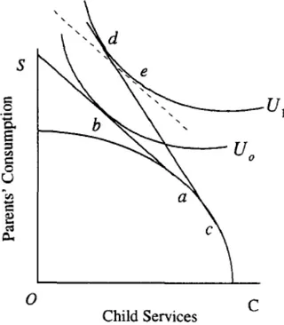
frac-Figure 1.3 – Effect of an increase in the female wage

tion of married life devoted to market work.

The major empirical hypotheses of this static model are developed from comparative static analysis of the effects of exogenous variations in husband’s income and female wage rates on fertility choices and related labour supply decisions by the wife. These results are presented diagrammatically in Fig.1.3 for an increase in the wife’s market wage, w, and for an increase in the husband’s income, H, in Fig.1.4.13

An increase in w causes for wives a shift from point a to point c on the production frontier in Fig.1.3 so that the linear portion of the new frontier (L > 0) is outside of and steeper than the linear portion of the previous frontier. It implies that the increase in w increases the household’s real income and increases the opportunity cost of children and the household moves its optimal choice from point b to point d. The total effect of the increase in w on c is ambiguous because the substitution effect against c be more than offset by a positive income effect in favor of c. Even if the income effect dominates so that c = nq increases, it is possible that fertility decreases while child quality increases. Indeed, Willis (1973) argues that this may be the probable outcome because it seems unlikely that child quality would

(29)

decrease while parents’ standard of living increases sharply. Thus, increases in the female wage might tend to attract increasing numbers of women into the labour force and reduce fertility at high parities while, at the same time, it reduces the incidence of childlessness among women who have the lowest levels of fertility.

Although the income effect associated with increasing female wages may push women away from childlessness toward married lives in which they combine motherhood and work, this effect may be offset by increasing returns to human capital investments in labour market careers caused by the fact that the returns to a given investment in human capital are proportional to its rate of utilization. To the extent that rising female wages lead women to devote a larger fraction of their lives to market work, there is a larger return to investments for women in market-related skills and reinforcing effects on their incentive to supply market labour and on the shadow price of time.14

As shown by Willis (1973), investment in wife’s human capital leads to a non-convex production possibility frontier which decreases the likelihood that a mix of motherhood and market work will dominate corner solutions involving either high fertility and specialization in home work or childlessness and an emphasis on the wife’s labour market career.

As far as the husband’s income is concerned, under the assumption of chil-dren as relatively time-intensive goods, its increase will have an asymmetric effect on the household’s production frontier, increasing the potential output of adult commodities by more than it increases the potential for child-related commodities, when the wife’s supply of time is held constant (Fig.1.4). If the household’s preferences for children are relatively weak and the wife sup-plies a positive amount of market labour when husband’s income is low, an increase in income will cause her to reduce her supply of labour. As long as she continues work at a constant wage, her price of time remains constant and, consequently, the opportunity cost of children also remains constant. Thus, in this case, the increase in H leads to a pure income effect which presumably increases the demand for c, and, because of quality-quantity in-teractions, has an ambiguous effect on the demand for number of children. For households with the same initial resources and a demand for c which is sufficiently strong that the wife does not work, the income effect result-ing from an increase in H tends to be offset by a substitution effect against children, moving the equilibrium from point a to point c in Fig.1.4. It is more likely that increases in husband’s income will reduce fertility among

14_{The enormous literature on investments in human capital by women originates with}

Mincer and Polachek (1974) and the emphasis of the effects of increasing returns on the sexual division of labour is found in Becker (1991).

(30)

Figure 1.4 – effect of an increase in the husband’s income

(31)

Features of life-cycle models of fertility and the optimal solution

1.3 Dynamic life-cycle models of fertility

This section presents the crucial features of the dynamic, or life-cycle, models of fertility that have been developed in the literature: changes in prices and income over the life cycle may result in changes in the timing of fertility demand or fertility tempo (even if they do not affect the choice of fertility quantum). Furthermore, the life-cycle framework is also the proper setting to insert the stochastic process of human reproduction, including the choice of contraceptive practices, and to examine the relationships between women’s labour supply, investment in human capital and childbearing decisions.15

1.3.1 Features of life-cycle models of fertility and the optimal so-lution

Following Hotz et al.(1997), I consider a household which consists of a woman and her spouse as a unique decision maker to make fertility and time and resource allocation decisions over a finite lifetime, characterize their lifetime in discrete time units t that index the age of the household unit and their lifetime runs from zero to T.16 Under a ratioanl choice perspective, it as-sumes that the couple make their choices to maximize a well-defined set of preferences, subject to time and financial budget constraints, to technological constraints (which rule the (re)production and rearing of children), and to constraints on the production of the woman’s stock of human capital (which determines the value of her time in the labour market at each age). The couple will make these decisions either in a certain or an uncertain setting, where the uncertainty they may face can arise either from the stochastic na-ture of the reproductive process or of the funa-ture income, prices or wage rates they may face.

Preference structures and the production of child services

As the structure of preferences within the static models, the most general specification of lifetime parental utility function considered in the literature takes the form:

15_{Hotz et al.(1997, p.309) argue: “Existing economic theories of fertility in a life-cycle}

setting blend features of static models of fertility with those from at least four different strands of dynamic models of behavior: (i) models of optimal life-cycle consumption, (ii) models of life-cycle labour supply decisions, (iii) models of human capital investment and accumulation, and (iv) stochastic models of human reproduction”.

16_{An exception to the rule is Hotz and Miller (1986) model in which couples are assumed}

(32)

U =

T

X

t=0

βtu(ct, lt, st) (1.9)

where lt is the amount of time the mother consumes in leisure activities

at age t, s is parental consumption, β is the couple’s rate of time preference (0 ≤ β ≤ 1), and ct the flow of child services parents receive at age t from

their stock of children, is ruled by the following production process:

ct= (b0, b1, ..., bt−1, tct, xct) (1.10)

where bτ = 1 if the parents had a childbirth when they were age τ (τ =

0, ..., t − 1) and bτ = 0 otherwise, and tct and xct denote, respectively, the

mother’s time and a vector of inputs used by child services (that includes also non-parental child-care services); then, the couple’s stock of children at age t is given by nt= t−1 X τ =0 bτ (1.11)

In the literature, the life-cycle models of fertility differs each other (and from this framework) in terms of several specializations: the simplest specifi-cation is Happel et al. (1984) that assumes that U in Equation (1.9) does not depend on ltat any age and does not depend on ctexcept at age T, when child

services are assumed to be proportional to nT, the couple’s completed family

size (cT = nT). The majority of the studies of the life-cycle models developed

to date, child services c(.) vary with the parents’ age but are restricted to be proportional to the accumulated number of children nt. The exceptions

are the papers by Moffitt (1984) and Hotz and Miller (1986) in which in the specifications of Equation (1.10) parental time inputs tct, and market inputs

xctvary as a function of the ages of children, with young children “requiring”

more maternal time and older children more market inputs. Maternal time constraints

The life-cycle models include period-by-period constraints on the mother’s time of the form

(33)

Features of life-cycle models of fertility and the optimal solution

lt+ ht+ tct= 1 (1.12)

where it uses to normalize the per-period amount of time available to the mother to one and where ht is the (normalized) amount of time she spends

in the labour market.17

Production of children

In the literature, as in the static models of fertility assumed that the control of fertility was perfect and costless, this assumption is recalled by several of the life-cycle models, such as Wolpin (1984), Moffitt (1984), Happel et al. (1984), and Cigno and Ermisch (1989). But, as argued by the demographic and biological literature, controlling a woman’s fertility is not likely to be either perfect or without costs in terms monetary or psychic. Thus, Heckman and Willis (1975) started to model human reproduction as a stochastic process in which childbirth represents a realization of this one. The models developed by Rosenzweig and Schultz (1985) and Hotz and Miller (1988) also incorporate the stochastic nature of reproduction into choice based, life-cycle models of fertility and build a couple’s fertility function like stochastic but controllable, in part, by the contraceptive strategies they choose:

bt= R(et, ϕt) (1.13)

where btis a random variable, etdenotes a K-dimensional vector in which

the ek element is whether or not the k th contraceptive method is used with

k = 1..., K and ϕtdenotes the stochastic component of the likelihood to have

a childbirth that a birth is produced with an unprotected sexual act. The parents’ birth probability function is given by

Pbt(et, µ, σ2φ) ≡ P r(bt= 1 | t, et, µ, σ2φ) = Eφ(R(et, ϕt) (1.14)

where Eφ(.) denotes the expectations operator over the random variable

ϕt, µ is its mean that measures the couple’s fecundty and σφ2 denotes its

variance. In this way, models in which the birth process is stochastic, as in Equation (1.13), transform the parents’ intertemporal optimization problem into one of decision making under uncertainty.

17_{To my knowledge, not exist life-cycle models consider the time allocation decisions of}

fathers, they are assumed only to provide for the rearing of children through the income they generate.

(34)

The household’s budget constraint

The scholarship of life-cycle models of fertility presents two assumptions about budget constraints that vary in base on the parents’ ability to save and/or their access to capital markets: the capital markets are assumed ei-ther perfect (PCM) in which parents are able to borrow and lend across time periods at a real interest rate r, or perfectly-imperfect (PICM), in which cap-ital market is not available to borrowings or savings. In the first case, PCM assumption, savings at time t is counted by St ≡ At− At−1 where At is the

parents’ assets can be borrowed or lent over time, and the parents’ budget constraint at time t is given by

St = Yht+ wtht− st− pct0 xct− p0etet− πnnt (1.15)

where Yhtdenotes husband’s income at time t, wtis the wife’s market wage

rate, pct and pet are vectors of prices for market inputs to the production of

child services and the out-of-pocket costs of contraceptives, respectively, and πn denotes the per unit non-quality cost of children. A key feature of the

PCM assumption is that savings in any period can be positive or negative, so parents are allowed to borrow against the future or dissave.18

In the second case of PICM assumption,19 _{parents cannot save, S} t = 0

for all t, and parental consumption is constrained by the following period by period constraint:

Yht+ wtht= st+ p0ctxct+ p0etet+ πnnt (1.16)

Finally, considering parental decision making within the life-cycle context puts the possibility that they face uncertainty about future income and prices: most of the literature on life-cycle fertility does not incorporate this form of uncertainty, while the model of Hotz and Miller (1988) in which future realizations of husband’s income Yht and the wife’s wage rate w are treated

as stochastic.

18_{See Happel et al. (1984), Moffitt (1984), and Walker (1995) that have this assumption}

about capital markets.

19_{The models of Heckman and Willis (1975), Wolpin (1984), and Hotz and Miller (1988)}

(35)

The optimal timing of motherhood

Maternal investments in human capital

In most of the models in which the allocation of maternal time is treated as endogenous, the mother’s wages over her life cycle are treated as exogenously determined. However, the models of Happel et al. (1984), Moffitt (1984), Cigno and Ermisch (1989) and Walker (1995) incorporate the possibility of maternal human capital investment, as such the mother’s participation in the labour force not only generate income for the family but also may enhance her future labour market skills, and thus her future wage rate possibilities. This is an important feature because it introduces a potentially important source of intertemporal variation in the opportunity cost of maternal time in the production and care of children and, thus, in the timing of births over the life cycle.

The life-cycle fertility models which introduce human capital investment generally adopt a “learning-by-doing” human capital production process in which maternal wage rates are determined, in part, by the mother’s past labour supply and her current work effort. More formally, this production function is given by

wt= H(wt−1, ht) − δ1wt−1− δ2wt−11[ht= 0] (1.17)

where H(·, ·) is the human capital production function, 1[·] is the indicator function, and δ1 and δ2 are rates of depreciation (0 ≤ δi ≤ 1, i = 1, 2) of

woman’s skills and, thus, her subsequent wage rates, due to not use in the labour market.

1.3.2 The optimal timing of motherhood

In this section life-cycle dynamic models identify on the one hand consump-tion smoothing, and on the other hand career planning of the woman as the main explanations to the fertility choices. Following Gustafsson (2001),I describe three theoretical models, such as Happel et al.(1984), Cigno and Ermish (1989), and Walker (1985), in detail to summarize the main findings of this literature.

Happel et al. (1984) assume consumption smoothing as the major deter-minant of fertility timing. Individual utility is separable into consumption and the ‘effective’ number of children, like a combination of quantity and quality. Under PICM assumption, the husband’s (exogenous) earnings pro-file matters for fertility timing since women give birth in a time spell in which the primary earner income is relatively high. The wife’s earnings depend on

(36)

pre-marital work experience and when she gives birth she retires from the labour market for a fixed exogenous period, during which job skills subject depreciation and obsolescence. The optimal time to have the first child is husband’s income reaches the highest peak; the household smoothes its con-sumption profile and raises its economic welfare delaying the childbirth (and the wife’s periods of inactivity in the labour market). Thus, the polices which aim to reduce the out of work time for women could tackle this postponement effect.

On the contrary, Cigno and Ermish (1989), also presented in Cigno (1991) put the career planning motive as the main determinant of LFP and fertility choices. Parents’ utility is disagregated into consumption and ‘effective’ chil-dren. Parents have a positive discount rate and PCM assumption. In based on this model a higher of pre-marital human capital stock implyes a lower completed fertility in the number and early child births. This is due to the income effect, in fact parents discount the utility come from offspring. He suggests that women with a steeper earnings profile postpone child births: in fact, for a steep earnings profile the current cost is relatively lower when a woman is young, while the future cost decreases with age since there are less years of work activity left.

Finally, under PCM assumption, Walker (1995) focuses on the career planning motive, and he specifies a dynamic model in which parents derive utility from children and consumption. The parents are strongly encouraged to have children early in the life-cycle due to the fact that children yield a recursive flow of utility also for all periods following the birth event, which is discounted at a positive rate of time preference (unlike in Happel et al. 1984): the motivation is that during a period of increasing wages, ceteris paribus, women have an incentive to give birth early in the life-cycle, when the oppor-tunity cost of their time is relatively low. The current wage forgone derived by birth and rearing children is much lower when an individual is relatively younger. In this model an increase in wealth tends by the cumulative nature of the utility flows to reduce the tempo of fertility too, while, by contrast, changes which flatten the earnings profile tend to delay fertility.

1.3.3 The optimal spacing of motherhood

The econometric Timing and Spacing literature is born by the hypothesis of a negative effect of female wages and a positive effect of male wages on fertility (Butz and Ward 1979; Heckman and Walker 1990; Tasiran 1995; Merigan and St Pierre 1998). The dependent variable collapses all the different features of the development of the fertility rates into one measure, the hazard rate.

(37)

The optimal spacing of motherhood

choices, sterility, childlessness, interbirth intervals and initiation of preg-nancy with in a unfied framework” in order to distinguish between tempo of fertility (the age at first birth) and quantum of fertility (the number of children born). Their another contribution is given by the estimation of birth transitions by a method that the literature call ‘a piecemeal approach of estimating one birth transition at a time’ that account for unobserved heterogeneity between individual women’s fertility. They consider this unob-served heterogeneity as a measure of individual differences in fecundity, but they also claim that: “Unlike for societies like the Hutterites where serially correlated fecundity differences play a central role, in accounting for fertility in modern Sweden serially correlated unobservables play a negligible role” (Heckman and Walker 1990, p. 235) because in modern European societies with low fertility rate we would expect that economic variables would play a more decisive role. They (1990) use current wages of males and females to explain fertility transitions and motivate this choice by the fact that “the correlation between past, current and future wages is very large, which makes current wages a good prediction for future wages”. and they find that there are signficant positive effects of male wages and significant negative effects of female wages in Sweden; these results are confirmed also in the study of Canadian fertility by Merrigan and St Pierre (1998) .

Tasiran (1995) analysing timing and spacing of births in Sweden using basically the same dataset as (Heckman and Walker 1990) (SFS) matching the Swedish household panel dataset (HUS) gets results that contrast: in fact, he finds much weaker effects of current male and female wages on birth transitions. The differences in results could be due to the fact that he uses individual observations on wages in a larger time series of aggregate male and female wages and adds other explanatory variables, such as parental benefits and child-care into the hazard models.

Adser`a (2011) estimates proportional hazard models of the transitions to the first three births using individual level data from the European Commu-nity Household Panel (ECHP). She controls for several time-varying measures of country-specific aggregate market conditions, such as unemployment rates, shares of public sector and part time employment, as covariates of interest in order to investigate the association between labour market dynamics and fertility choices. This study shows that high and persistent unemployment rate of the country is associated with delays in childbearing and, as a result, a likely lower number of children. For a given unemployment level, a wide supply of public sector employment yields a faster transitions to all births, while second births occur sooner in countries where the access to part-time makes it easy. Finally, women with temporary contracts, mostly prevalent in Southern Europe, are the least likely to give birth to a second child.

(38)

Finally, Bratti and Tatsiramos (2012) focus on the consequences of delay-ing motherhood on fertility in several European countries usdelay-ing the European Community Household Panel (ECHP). Estimating a multistate discrete-time duration model, which accounts for correlated unobserved heterogeneity across parities, they are able to analyze the effect of age at first birth on the tran-sition to the second parity, addressing jointly the endogeneity of age at first birth. The empirical study shows the coexistence of two opposite forces, the biological and sociocultural factors producing a postponement effect and career-related factors leading to a catch-up effect. Their magnitudes vary and depend on countries’ institutional features: in particular, the postpone-ment effect is larger in Southern European countries, where a traditional male-breadwinner model prevails and where it is not favored the concilia-tion between family and work, while a catch-up effect is large in countries where institutions support properly the mothers to participate in the labour market.

(39)

Empirical implications of models of fertility: identification issues

1.4 Empirical implications of models of fertility:

iden-tification issues

While there is strong and recent evidence on the negative effect of child bearing on female labour supply and vice versa, the interpretation of this correlation is complicated by several modelling issues.

Firstly, there may be an endogeneity issue arising from the presence of unobservable factors that may affect both the participation and fertility de-cisions (Browning1992). For instance, women with stronger preferences for a career-based life style may have fewer children and may also have higher unobservable skills in the labour market. In this case, the observed negative relationship between fertility and employment could be spurious. The endo-geneity of fertility choices has been tackled by exploiting exogenous changes in the family composition. One of the proposed instruments is the sex of the first two children, as parents with two children of the same sex are more likely to be willing to have a third child (Angrist and Evans 1998; Carrasco 2001). Alternatively, exogenous infertility shocks, based on information on the use of contraceptives, have recently been used as instruments to iden-tify the causal effect of having children on female labour supply (Ag¨uero and Marks 2008). While the latter strategy has the advantage of being applicable to a broader sample of women in fertility age, the former uses information on family composition that can be easily found in households surveys.

Secondly, part of the literature on life-cycle labour supply has treated employment and fertility as a result of a joint dynamic process, to explicitly account for the effect of past labour supply and existing children on present participation and fertility choices. This strand of literature has considered fertility as predetermined in a sequential dynamic framework (Arellano and Carrasco 2003; Michaud and Tatsiramos 2011) or as contemporaneous with respect to labour market participation decisions (Del Boca 2002; Francesconi 2002; Del Boca and Sauer 2009; Keane and Sauer 2009; Eckstein and Lif-shitz 2011). In addition, further to the distinction between genuine state dependence and permanent unobserved individual effects, the literature on dynamic labour supply has recently emphasised the importance of accounting for autocorrelation in time-varying unobserved heterogeneity. In fact, Hys-lop (1999), following Browning (1992) and Chamberlain (1984), tests for the exogeneity of fertility via a discrete choice correlated random effects model. His results indicate that fertility is endogenous when dynamic factors such as state dependence or serial correlation are excluded. Thus, in dynamic specifications including either first-order state dependence or AR(1) serial correlation, he finds no unambiguous evidence against the exogeneity of

(40)

fer-tility hypothesis. Directly testing for the exogeneity of ferfer-tility has yielded very mixed results.