Border Collision Bifurcations in a Generalized Model of Population Dynamics

(1)

Research Article

Border Collision Bifurcations in a Generalized Model of

Population Dynamics

Lilia M. Ladino,

1

Cristiana Mammana,

2

Elisabetta Michetti,

2

and Jose C. Valverde

3

1_{Department of Mathematics and Physics, University of Los Llanos, 500001 Villavicencio, Colombia}

2_{Department of Economics and Law, University of Macerata, 62100 Macerata, Italy}

3_{Department of Mathematics, University of Castilla-La Mancha, 02071 Albacete, Spain}

Correspondence should be addressed to Cristiana Mammana; cristiana.mammana@unimc.it

Received 21 December 2015; Revised 24 February 2016; Accepted 22 March 2016

Academic Editor: Xiaohua Ding

Copyright © 2016 Lilia M. Ladino et al. This is an open access article distributed under the Creative Commons Attribution License, which permits unrestricted use, distribution, and reproduction in any medium, provided the original work is properly cited.

We analyze the dynamics of a generalized discrete time population model of a two-stage species with recruitment and capture. This generalization, which is inspired by other approaches and real data that one can find in literature, consists in considering no restriction for the value of the two key parameters appearing in the model, that is, the natural death rate and the mortality rate due to fishing activity. In the more general case the feasibility of the system has been preserved by posing opportune formulas for the piecewise map defining the model. The resulting two-dimensional nonlinear map is not smooth, though continuous, as its definition changes as any border is crossed in the phase plane. Hence, techniques from the mathematical theory of piecewise smooth dynamical systems must be applied to show that, due to the existence of borders, abrupt changes in the dynamic behavior of population sizes and multistability emerge. The main novelty of the present contribution with respect to the previous ones is that, while using real data, richer dynamics are produced, such as fluctuations and multistability. Such new evidences are of great interest in biology since new strategies to preserve the survival of the species can be suggested.

1. Introduction

Mathematical systems modeling natural phenomena usu-ally depend on parameters related to their behavior. The determination of the essential parameters and their possible values is fundamental not only for the design of an adequate model, but also for the prediction of the evolution of these phenomena in the future.

The dynamics of a system can change drastically as the parameters vary, providing different kinds of evolution. Such changes in the dynamics are known as bifurcations and they have become a very interesting subject in the study of dynamical systems, a field in which many researchers have worked in the last years (see, e.g., Kuznetsov [1] or Balibrea et al. [2], Yuan et al. [3], Franco and Per´an [4], and references therein).

Actually, these parameters can force the design of the model in order to maintain the empirical meaning, providing piecewise systems (see Simpson [5] for a wider description of piecewise smooth systems and the related bifurcations).

Piecewise smooth dynamical systems are of great interest in many areas of applied science since they show a large variety of nonlinear phenomena including chaos. While there is a complete understanding of local bifurcations for smooth dynamical systems, nonstandard bifurcations are likely to emerge in piecewise smooth dynamical systems. An analyti-cal study regarding bifurcations in such kind of systems firstly appeared in Feigin [6]. Later, the results due to Feigin have been formalized within the context of modern bifurcation analysis in Di Bernardo et al. [7]; in that work the effects of such bifurcations are described and the related conditions are pursued. More in detail, when a piecewise smooth system is considered, the exhibited dynamics could vary when an invariant set, for example, a cycle or a fixed point, collides with a switching manifold. When these variations in the dynamics occur, it is said that the system undergoes a

border collision bifurcation. Many authors have carried out

researches on these kinds of bifurcations in the last decades (see, e.g., Nusse and Yorke [8], Brianzoni et al. [9], Simpson and Meiss [10], Agliari et al. [11], and the references therein).

Volume 2016, Article ID 9724139, 13 pages http://dx.doi.org/10.1155/2016/9724139

(2)

In a previous work [12], we studied a discrete time continuous and differentiable dynamical system in biology, which models the population dynamics of a two-stage species with recruitment and capture. In such work, to be coherent with the biological meaning of the model, the possible values of the essential parameters are determined by two nonnegative constraints under which the dynamics of the discrete model considered coincide exactly with its contin-uous counterpart analyzed in Ladino and Valverde [13]. In both the discrete and continuous models, the system exhibits a transcritical bifurcation while one of the equilibria is a global attractor of the system (alternatively), depending on the value of a threshold parameter which is a function of the key parameters. No richer dynamics are exhibited.

Nevertheless, in literature (e.g., see CCI and INCODER [14]), one can find other approaches in which the parameters considered in the definition of the model do not satisfy the constraints given in Ladino et al. [12]. This issue has motivated us to study, in this work, what happens when the parameters are not restricted by such constraints, thus considering real data for two species. In particular, for nonrestricted parameter values, the (discrete) system can be reformulated by a piecewise nonlinear map for it to continue to be mathematically coherent.

To better explain, in the present contribution we consider the model proposed in Ladino and Valverde [13] (which is a two-dimensional model in continuous time) and we obtain its discrete time formulation by considering the variation of each state variable in a unit time. Even if this is a simplified manner to obtain the discrete counterpart of the initial model, we proceeded in such a way for the following main reasons. First of all, this contribution represents the first step in the study of the dynamics of exploited populations, when time is assumed to be discrete and real data are taken into account; hence we chose to start considering its basic initial formulation. Secondly, the main goal of the present work is to easily compare the results herewith obtained to the ones reached in the equivalent continuous time model. Finally, new and more accurate discrete time setups could be proposed in further developments and thus compared to the present one, in order to conclude about their strength and weakness points when used to describe real situations.

Once obtained the discrete time system to be studied, we explicitly take into account that nonnegativity constraints

must be considered. In fact, if at a given time 𝑡 + 1 ∈

N a state variable becomes negative, this means that the recruitment and capture processes have affected the whole related subpopulation, and hence such a subpopulation must be assumed to be equal to zero. Due to the nonnegativity constraints, the final model is described by a continuous two-dimensional piecewise smooth map. Actually, borders may appear in the phase plane where the definition of the dynamic system changes. As a consequence, the approach to the problem requires the use of new techniques from the mathematical theory of piecewise smooth dynamical systems as well as computational support (recent works of this kind are, among others, Kubin and Gardini [15], Banerjee and Grebogi [16], and Simpson [17]).

We recall that piecewise smooth systems are able to exhibit the same dynamics as those produced in smooth systems but, in addition, new phenomena related to the existence of borders may be produced (see Simpson [5]). In fact, it may occur that, when a border is crossed, a different kind of bifurcation that is not related to the eigenvalues associated with a given attractor, called border collision bifurcation, may emerge (Nusse and Yorke [8, 18]). This type of bifurcation is of great relevance from an applied point of view, since the eigenvalues of fixed or periodic points play no role and, consequently, it is more difficult to predict if a system is close to a border collision bifurcation and it is more difficult to predict what happens to the qualitative nature of the attractor after the border collision bifurcation. The latter difficulty is reinforced by the fact that, after a border collision bifurcation, coexisting additional attractors often occur, so that the related basins of attraction have to be considered.

As models in applied mathematics often consider con-straints (such as capacity concon-straints in biology or resource constraints in economics, etc.), piecewise smooth dynamical systems emerge quite naturally in applications and conse-quently their study has been improved in recent years (see, e.g., Agliari et al. [11], Brianzoni et al. [9], Simpson and Meiss [10], and Sushko et al. [19]). Nevertheless, such works usually focus on the local bifurcations related to periodic points and other attractors, while the global dynamics are mainly described using numerical techniques.

We will follow this approach also in the present paper but, in addition, (1) we will be able to reach some results on the global dynamics of the system and (2) we will apply our findings to two real cases. In fact, for the numerical simula-tions, we will consider actual data related to the population parameters on the state of fisheries for two fish species, that is, Prochilodus mariae and Prochilodus magdalenae, which inhabit in the Orinoco and Magdalena rivers of Colombia (CCI and INCODER [14]). As far as the other parameters of the model are concerned, because of the difficulty of finding related serious research publications, we consider the values theoretically estimated in Ladino and Valverde [13]. Although using real data for the parameters would be of great interest, the numerical analysis we perform has the advantage of allowing us to simulate and analyze different scenarios of the feasible biological parametric space.

The paper is organized as follows. In Section 2, we describe the model of population dynamics; in particular, by considering nonnegativity constraints we obtain the final

two-dimensional system(𝑇, R2₊) whose evolution operator is

continuous and piecewise smooth. In Section 3, we describe the structure of borders and deal with the question of the existence and local stability of fixed points. In Section 4 the global dynamics is studied. More precisely, we show that the system admits an attractor at finite distance and that the extinction equilibrium is the unique global attractor under certain parametric conditions; we also show that the system undergoes a border collision bifurcation in which a 2-period cycle appears and that the model also exhibits a multistability phenomenon which plays an important role in the study of the evolution of the system. Section 5 concludes the paper

(3)

emphasizing the most important features of our research in terms of strategies to be suggested for the conservation of the species.

2. The Model

In Ladino et al. [12], the population dynamics of a two-stage species with recruitment and capture is modeled by the following system of nonlinear difference equations:

𝑥 (𝑡 + 1) = 𝑥 (𝑡) + 𝛿𝑦 (𝑡) −_{𝛽 + 𝑥 (𝑡)}𝛼𝑥 (𝑡) − 𝜇𝑥 (𝑡) ,

𝑦 (𝑡 + 1) = 𝑦 (𝑡) +_{𝛽 + 𝑥 (𝑡)}𝛼𝑥 (𝑡) − (𝜇 + 𝐹) 𝑦 (𝑡) ,

(1)

where all the parameters are nonnegative and verify the following two constraints:

𝜇 + 𝛼_𝛽≤ 1,

𝜇 + 𝐹 ≤ 1

(2)

in order to have biological significance. However, empir-ical studies [14] estimated parameter values that do not necessarily verify the abovementioned constrains. For this reason, in this work we present a generalization of system (1), where the parameters do not necessarily verify the constraints above. In this sense, we will need to reformulate the model as a piecewise nonlinear map for it to maintain biological significance.

By taking into account system (1), the two-dimensional system that characterizes the dynamics of a two-stage species with recruitment and capture can be rewritten as

𝑇1: { { { { { 𝑥󸀠_{= 𝑓 (𝑥, 𝑦) = (1 − 𝜇) 𝑥 + 𝛿𝑦 −} 𝛼𝑥 𝛽 + 𝑥, 𝑦󸀠_{= 𝑔 (𝑥, 𝑦) = (1 − 𝜇 − 𝐹) 𝑦 +} 𝛼𝑥 𝛽 + 𝑥, (3) where 𝑥󸀠 = 𝑥(𝑡 + 1), 𝑥 = 𝑥(𝑡), 𝑦󸀠 = 𝑦(𝑡 + 1), and

𝑦 = 𝑦(𝑡). System 𝑇1is a two-dimensional dynamical system

whose iteration defines the time evolution of the prerecruit

population𝑥 and the exploitable population 𝑦.

First of all, we observe that system (3) is biologically

meaningful only when, at any time𝑡, the two states variables

𝑥 and 𝑦 belong to R2

+.

It is quite immediate to verify that not all trajectories

produced by system𝑇₁are feasible for all parameter values.

For instance, an initial condition(0, 𝑦(0)), 𝑦(0) > 0 produces

an unfeasible trajectory if𝜇 + 𝐹 > 1 or, similarly, a trajectory

starting from(𝑥(0), 0) exits from R2₊ at the first iteration if

𝜇 > 1.

Nevertheless, it can be observed that, if at a given time 𝑡 ∈ N one of the two subpopulations becomes negative, that

is,𝑥(𝑡) < 0 or 𝑦(𝑡) < 0, then this fact implies that, at some

earlier time, the subpopulation evolved into its extinction and therefore its size must be assumed to have become equal to zero. More in detail, nonnegativity constraints must be taken

into account in order to consider that the natural death rate𝜇

and the capture mortality rate𝐹 can affect, at most, the whole

stock of a subpopulation.

As a consequence, we can define the following systems:

𝑇2: { { { 𝑥󸀠_{= 0} 𝑦󸀠_{= 𝑔 (𝑥, 𝑦) ,} iff 𝑓 (𝑥, 𝑦) < 0, 𝑔 (𝑥, 𝑦) ≥ 0, (𝑥, 𝑦) ∈ R2₊, 𝑇3: { { { 𝑥󸀠_{= 0} 𝑦󸀠_{= 0,} iff 𝑓 (𝑥, 𝑦) < 0, 𝑔 (𝑥, 𝑦) < 0, (𝑥, 𝑦) ∈ R2₊, 𝑇₄:{_{ { 𝑥󸀠_{= 𝑓 (𝑥, 𝑦)} 𝑦󸀠_{= 0,} iff 𝑓 (𝑥, 𝑦) ≥ 0, 𝑔 (𝑥, 𝑦) < 0, (𝑥, 𝑦) ∈ R2₊, (4)

which describe the dynamics of the two subpopulations in

the case in which the prerecruit population vanishes(𝑇₂) or

the exploitable population vanishes(𝑇₄), or finally, the species

becomes extinct(𝑇₃).

System (1) can be now reformulated as

𝑇 = { { { { { { { { { { { { { { { 𝑇₁, iff (𝑥, 𝑦) ∈ 𝑈₁ 𝑇₂, iff (𝑥, 𝑦) ∈ 𝑈₂ 𝑇3, iff (𝑥, 𝑦) ∈ 𝑈3 𝑇4, iff (𝑥, 𝑦) ∈ 𝑈4, (5) where 𝑈1= {(𝑥, 𝑦) ∈ R2+ : 𝑓 (𝑥, 𝑦) ≥ 0, 𝑔 (𝑥, 𝑦) ≥ 0} , 𝑈₂= {(𝑥, 𝑦) ∈ R2₊ : 𝑓 (𝑥, 𝑦) < 0, 𝑔 (𝑥, 𝑦) ≥ 0} , 𝑈₃= {(𝑥, 𝑦) ∈ R2₊ : 𝑓 (𝑥, 𝑦) < 0, 𝑔 (𝑥, 𝑦) < 0} , 𝑈4= {(𝑥, 𝑦) ∈ R2+ : 𝑓 (𝑥, 𝑦) ≥ 0, 𝑔 (𝑥, 𝑦) < 0} . (6)

Notice that system (𝑇, R2₊) is not smooth, since its

definition changes, though continuously, as any border is

crossed in the phase plane(𝑥, 𝑦), due to the nonnegativity

constraints.

3. Fixed Points and Local Stability

3.1. Preliminary Properties. As it has been described, the

phase plane is divided into several regions,𝑈_𝑖(𝑖 = 1, 2, 3, 4),

and system𝑇 is defined in different ways inside each of them.

As a first step in the analysis, we want to better describe

the structure of such regions on the planeR2₊, depending on

the parameters of the model. The following lemma can be proved.

(4)

Lemma 1. Let 𝑇 be given by (5) and 𝑈_𝑖, 𝑖 = 1, 2, 3, 4, as

defined in (6). Then the following statements hold:

(i) if𝜇 + 𝐹 ≤ 1, then 𝑈₃and𝑈₄are empty;

(ii) if𝜇 + 𝛼/𝛽 ≤ 1, then 𝑈₂and𝑈₃are empty.

Proof. (i) Consider a point(𝑥, 𝑦) ∈ R2₊. Then(𝑥, 𝑦) belongs

to𝑈₃or to𝑈₄iff𝑔(𝑥, 𝑦) < 0. Let 𝜇 + 𝐹 = 1; then condition

𝑔(𝑥, 𝑦) > 0 cannot hold. Hence we consider the case 𝜇+𝐹 < 1

and observe that𝑔(𝑥, 𝑦) < 0 iff 𝑦 < 𝑔₁(𝑥) = −𝛼𝑥/(𝛽 + 𝑥)(1 −

𝜇−𝐹). Notice that 𝑔₁(0) = 0; furthermore if 1−𝜇−𝐹 > 0 then

lim_𝑥→+∞𝑔₁(𝑥) < 0 and 𝑔󸀠₁(𝑥) = −𝛼𝛽(1 − 𝜇 − 𝐹)/[(𝛽 + 𝑥)(1 −

𝜇 − 𝐹)]2_{< 0 (i.e., 𝑔}

1is strictly decreasing). As a consequence

𝑦 ≥ 𝑔₁(𝑥), ∀𝑥 ≥ 0 and the statement is proved.

(ii) Consider a point(𝑥, 𝑦) ∈ R2₊. Then𝑓(𝑥, 𝑦) < 0 iff

𝑦 < 𝑓₁(𝑥) = 𝑥[(𝛽 + 𝑥)(𝜇 − 1) + 𝛼]/𝛿(𝛽 + 𝑥). Notice that

𝑓₁(0) = 0 and that if 𝜇 < 1 then lim_𝑥→+∞𝑓₁(𝑥) = −∞.

Assume𝜇 < 1 and consider that 𝑓₁󸀠(𝑥) = (𝛿(𝛽 + 𝑥)2(𝜇 − 1) +

𝛼𝛿𝛽)/[𝛿(𝛽 + 𝑥)]2. Then, after some algebra, it can be verified

that, if𝜇 + 𝛼/𝛽 ≤ 1, then 𝑓₁is strictly decreasing∀𝑥 ≥ 0 and

consequently condition𝑦 < 𝑓₁(𝑥) cannot hold. Therefore,

there is no point in𝑈₂nor in𝑈₃.

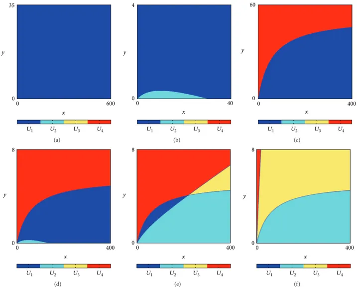
With the same arguments used in the proof of Lemma 1, it can be easily demonstrated that several situations can occur, depending on the parameters of the model. In particular, the following remark can be easily verified.

Remark 2. Let 𝑇 be given by (5) and 𝑈_𝑖, 𝑖 = 1, 2, 3, 4 as

defined in (6). Then,

(i) if𝜇 + 𝐹 ≤ 1 and 𝜇 + 𝛼/𝛽 ≤ 1, then 𝑈₁ = R2₊(see

Figure 1(a));

(ii) if𝜇 + 𝐹 ≤ 1 and 𝜇 + 𝛼/𝛽 > 1, then 𝑈₁∪ 𝑈₂= R2₊(see

Figure 1(b));

(iii) if𝜇 + 𝐹 > 1 and 𝜇 + 𝛼/𝛽 ≤ 1, then 𝑈₁∪ 𝑈₄= R2₊(see

Figure 1(c)).

Observe that the cases presented in Figure 1(c) are one of the cases studied in CCI and INCODER [14], that is, for the fish P. mariae.

It is important to observe that, for parameter values different to those considered in Remark 2, several situations may occur; that is, more than two regions are present on the

planeR2₊. The structure of such regions can be ambiguous,

since it is strictly related to the parameter values. In particular,

such situations emerge when𝜇 + 𝐹 > 1.

More precisely, let us consider 𝜇 + 𝐹 > 1, 𝜇 < 1, and

𝜇 + 𝛼/𝛽 > 1. Then, taking into account the arguments used

to prove Lemma 1, it can be observed that𝑈₁,𝑈₂, and𝑈₄

are not empty and that, for suitable values of the parameters,

also 𝑈₃ may appear (e.g., it depends on the comparison

between 𝑔󸀠₁(0) and 𝑓₁󸀠(0), where 𝑔₁ and 𝑓₁ are defined in

the proof of Lemma 1). Specifically, taking into account the parameter values used in CCI and INCODER [14] for the fish

P. magdalenae, the situation showed in Figure 1(d) occurs.

On the other hand, let us consider the case with𝜇 ≥ 1.

Then different scenarios may occur. In particular, if𝜇 > 1,

then the regions𝑈₂,𝑈₃, and𝑈₄are present, possibly together

with 𝑈₁. For instance, in Figure 1(e) the four regions are

present, while, with a lower value of𝛿, region 𝑈₁disappears,

as it is shown in Figure 1(f).

Summarizing, the phase space can have several regions

(up to four), where the map𝑇 takes on different definitions.

The different regions in the phase space are not uniquely determined, as they depend on the values of the parameters.

As a consequence, given the analytical form of 𝑇 and the

high number of parameters, it is difficult to predict the global behavior of the map from a given initial state. For this reason, new insights from the mathematical theory of piecewise smooth dynamic systems together with an empirical study must be used.

3.2. Extinction and Coexistence Equilibria. We now deal with

the question of the existence and number of fixed points of

system𝑇. The following proposition holds.

Proposition 3. Let system 𝑇 be given by (5).

(i) If𝜇 + 𝐹 < 𝛼𝛿/(𝜇𝛽 + 𝛼), then 𝑇 admits two fixed points

𝑃₀ = (0, 0) and 𝑃∗ _{= (𝑥}∗_{, 𝑦}∗_{) ∈ 𝑈} 1, with𝑥∗ > 0 and 𝑦∗ _{> 0, where} 𝑥∗= 𝛼 𝜇[ 𝛿 𝜇 + 𝐹− 1] − 𝛽, 𝑦∗= (_{𝜇 + 𝐹}1 ) (_{𝛽 + 𝑥}𝛼𝑥∗_∗) . (7)

(ii) If𝜇 + 𝐹 ≥ 𝛼𝛿/(𝜇𝛽 + 𝛼), then 𝑇 admits a unique fixed

point𝑃₀= (0, 0).

Proof. Let(𝑥, 𝑦) be a fixed point of system 𝑇₁. Then it must be 𝑓 (𝑥, 𝑦) = 𝑥 + 𝛿𝑦 − 𝛼𝑥 𝛽 + 𝑥 − 𝜇𝑥 = 𝑥, 𝑔 (𝑥, 𝑦) = 𝑦 + 𝛼𝑥 𝛽 + 𝑥− (𝜇 + 𝐹) 𝑦 = 𝑦, (8)

which implies that

𝛿𝑦 − 𝛼𝑥 𝛽 + 𝑥− 𝜇𝑥 = 0, (9) 𝑦 = 1 (𝜇 + 𝐹)( 𝛼𝑥 𝛽 + 𝑥) . (10)

By substituting𝑦 given by (10) in (9) we obtain

𝑥 [_{𝛽 + 𝑥}𝛼 (_{𝜇 + 𝐹}𝛿 − 1) − 𝜇] = 0. (11) Therefore 𝑥 = 0 or𝑥 = 𝛼 𝜇[ 𝛿 𝜇 + 𝐹− 1] − 𝛽 = 𝑥∗. (12)

(5)

0 600 0 35 x y U1 U2 U3 U4 (a) 0 40 0 4 x y U1 U2 U3 U4 (b) 0 400 0 60 x y U1 U2 U3 U4 (c) 0 400 0 8 x y U1 U2 U3 U4 (d) 0 400 0 8 x y U1 U2 U3 U4 (e) 0 400 0 8 x y U1 U2 U3 U4 (f)

Figure 1: The phase plane is divided into several regions depending on the parameters of the model. Some situations are depicted for different parameters values:𝑈₁is in blue,𝑈₂is in light blue,𝑈₃is in yellow, and𝑈₄is in red. (a)𝛼 = 20, 𝛽 = 60, 𝛿 = 14.6, 𝜇 = 0.5 and 𝐹 = 0.4; (b) 𝛽 = 10 and other parameters as in (a). (c) As in CCI and INCODER [14] for fish P. mariae, 𝜇 = 0.63, 𝐹 = 0.75 and other parameters as in (a). (d) As in CCI and INCODER [14] for fish P. magdalenae,𝜇 = 0.897, 𝐹 = 3.653 and other parameters as in (a). (e) 𝜇 = 1.2 and the other parameters as in (d). (f)𝛿 = 1 and the other parameters as in (e).

Note that if𝑥 = 0, then 𝑦 = 0. Therefore 𝑃₀ = (0, 0) is a fixed

point of system𝑇 for all parameter values.

Now assume that𝜇 + 𝐹 < 𝛼𝛿/(𝜇𝛽 + 𝛼). Then 𝑥∗ > 0.

Hence, in this case,𝑇 admits a second fixed point given by

𝑃∗_{= (𝑥}∗_{, 𝑦}∗_{) ∈ 𝑈}

1, that is,𝑥∗> 0 and 𝑦∗ > 0, where

𝑥∗= 𝛼 𝜇[ 𝛿 𝜇 + 𝐹− 1] − 𝛽, 𝑦∗= ( 1 𝜇 + 𝐹) ( 𝛼𝑥∗ 𝛽 + 𝑥∗) . (13)

Finally, it can be easily verified that no other fixed points exist

in𝑈₂,𝑈₃, and𝑈₄.

We will call𝑃₀extinction equilibrium and𝑃∗ coexistence

equilibrium. Notice that the extinction equilibrium exists for

all parameter values in order to have biological significance.

In fact, if at the initial time both subpopulations are equal to zero, then they will remain zero forever. Moreover, also the coexistence equilibrium is biologically significant, because its presence ensures that there is the possibility of the preservation of species over time.

Furthermore, let us consider

𝐹 = 𝛼𝛿

𝛼 + 𝜇𝛽− 𝜇; (14)

then, according to Proposition 3, it can be observed that

if 𝐹 > 0, the coexistence equilibrium exists as long as

𝐹 ∈ (0, 𝐹); that is, there is a limit value for the capture mortality of the species such that below this value the coexistence of both subpopulations is possible. With regard

to the localization of the coexistence equilibrium𝑃∗, note

that as𝐹 increases while approaching 𝐹, 𝑃∗ tends to(0, 0).

(6)

the coexistence equilibrium has an increasingly smaller size

for both subpopulations, while if𝐹 = 𝐹 the two fixed points

merge, thus giving rise to a bifurcation.

3.3. Local Stability. We now focus on the case in which

Remark 2(i) holds; that is,𝑈₁ = R2₊, so that𝑇 is defined by

𝑇₁,∀(𝑥, 𝑦) ∈ R2₊.

As far as the local stability of the fixed points is concerned,

we recall that the Jacobian matrix associated with𝑇₁is given

by 𝐽𝑇₁= ( 1 − 𝜇 − 𝛼𝛽 (𝛽 + 𝑥)2 𝛿 𝛼𝛽 (𝛽 + 𝑥)2 1 − 𝜇 − 𝐹 ) . (15)

Furthermore, following Medio and Lines [20], conditions

for the local stability of a fixed point𝑃 = (𝑥, 𝑦) are given by

(i)𝜑₁(𝑥) = (𝜇−2)2+(𝜇−2)𝐹+(𝜇+𝐹−𝛿−2)(𝛼𝛽/(𝑥+𝛽)2) >

0,

(ii)𝜑₂(𝑥) = 𝜇(𝜇 + 𝐹) + (𝜇 + 𝐹 − 𝛿)(𝛼𝛽/(𝑥 + 𝛽)2) > 0,

(iii)𝜑₃(𝑥) = −𝜇(𝜇 − 2) − (𝜇 − 1)𝐹 + (𝛿 − 𝜇 − 𝐹 + 1)(𝛼𝛽/(𝑥 +

𝛽)2_{) > 0.}

We recall that conditions (i), (ii), and (iii) guarantee the local

stability of𝑃 since they correspond, respectively, to 𝑃(−1) >

0, 𝑃(1) > 0, and (1 − det(𝐽𝑇1(𝑥))) > 0; that is, the roots

of the characteristic polynomial𝑃(𝜆) of the Jacobian matrix

evaluated at𝑃 are inside the unit circle.

The following proposition can be proved.

Proposition 4. Let 𝜇 + 𝐹 ≤ 1 and 𝜇 + 𝛼/𝛽 ≤ 1. If 𝜇 + 𝐹 >

𝛼𝛿/(𝜇𝛽 + 𝛼), then 𝑃0is locally stable.

Proof. Let𝜇 + 𝐹 ≤ 1 and 𝜇 + 𝛼/𝛽 ≤ 1 and consider system 𝑇₁

enlarged toR2, namely,𝑇₁₁. Then there exists a neighborhood

of the origin where𝑇₁₁is continuous and differentiable. In the

fixed point𝑃₀, condition (ii) is given by𝜑₂(0) = (𝐹 + 𝜇)(𝜇 +

𝛼/𝛽) − 𝛼𝛿/𝛽 > 0 corresponding to 𝜇 + 𝐹 > 𝛼𝛿/(𝜇𝛽 + 𝛼). So

assume that𝜇 + 𝐹 > 𝛼𝛿/(𝜇𝛽 + 𝛼).

Condition (i) is given by𝜑₁(0) = 𝜑₂(0) + 4 − 2(𝜇 + 𝐹) −

2(𝜇 + 𝛼/𝛽) > 0 while condition (iii) requires 𝜑₃(0) = 𝜇(2 −

𝜇) + 𝐹(1 − 𝜇) + (1 − 𝐹 − 𝜇 + 𝛿)(𝛼/𝛽) > 0. Both conditions are trivially verified under the posed conditions on parameters.

Hence𝑃₀is locally stable for system𝑇₁₁.

Consider now that system 𝑇₁, that is, 𝑇₁₁ restricted to

𝑈₁= R2

+, is not smooth in the origin; anyway, since Remark 2

holds, then𝑈₁ = R2₊ and 𝑇(𝑈₁) ⊆ 𝑈₁. Hence, since𝑃₀ is

locally stable for𝑇₁₁, it is also locally stable for system𝑇.

From a biological and fishery point of view, this result is relevant because as long as the initial conditions of the species are very small and have a combination of parameters such

that 𝜇 + 𝛼/𝛽 ≤ 1, then a set of parameter values can be

determined for which the capture mortality rate𝐹 is such that

the species is endangered and it evolves towards extinction;

that is, this occurs when𝛼𝛿/(𝜇𝛽+𝛼)−𝜇 < 𝐹 ≤ 1−𝜇. Therefore,

if the initial conditions of the species are very small and we

have the combination of parameters𝜇 + 𝛼/𝛽 ≤ 1, then it is

possible to regulate fishing so as to assure𝐹 < 𝛼𝛿/(𝜇𝛽+𝛼)−𝜇

in order to avoid species extinction. In fact, fishery policies may be adopted taking into account that fishing effort and catchability coefficient are the parameters that determine the capture mortality rate.

Notice also that taking into account Proposition 3, then if 𝐹 = 𝐹 one gets 𝜇 + 𝐹 = 𝛼𝛿/(𝜇𝛽 + 𝛼). The two fixed points

𝑃0 and 𝑃∗ merge since both𝐽𝑇1(𝑃0) and 𝐽𝑇1(𝑃∗) have an

eigenvalue equal to+1, thus giving rise to a border collision

for the map. Furthermore, it can be verified that if𝐹 < 𝐹, 𝑃∗

may be stable or already unstable before the merging, as it will be better explained in the following proposition concerning the local stability of the coexistence equilibrium.

Proposition 5. Consider 𝜇 < 1 and define 𝛽₁= 𝛼(2 − 𝜇)2_{(𝛿 −}

𝜇)2_/𝜇4_{(2 − 𝜇 + 𝛿).}

(i) Let𝐹 < 𝐹.

If𝛽 ≥ 𝛽₁, then𝑃∗is a saddle∀𝐹 ∈ (0, 𝐹).

If𝛽 < 𝛽₁, then two cases may occur:

(a)∃𝐹∗ ∈ (0, 𝐹) such that 𝑃∗ is locally stable

(resp., unstable)∀𝐹 ∈ (0, 𝐹∗) (resp., ∀𝐹 ∈

(𝐹∗_{, 𝐹)); at 𝐹 = 𝐹}∗_,_𝑃∗_{becomes a saddle;}

(b)𝑃∗is locally stable∀𝐹 ∈ (0, 𝐹).

(ii) At𝐹 = 𝐹, 𝑃₀and𝑃∗merge and two cases may occur:

(a) if𝛽 ≥ 𝛽₁,𝑃∗is a saddle before merging;

(b) if𝛽 < 𝛽₁, 𝑃∗ is locally stable or it is a saddle

before merging.

Proof. Consider𝜇 < 1 and 𝐹 < 𝐹. Then from Proposition 3,

𝑃∗ ∈ 𝑈₁and𝑥∗ > 0, 𝑦∗ > 0. It can be easily verified that

conditions𝛼𝛿 − (𝜇 + 𝐹)(𝛼 + 𝜇𝛽) > 0 and 𝛿 − 𝜇 − 𝐹 > 0 hold

and consequently 𝜑₂(𝑥∗) = 𝜇 (𝜇 + 𝐹) [𝛼𝛿 − (𝜇 + 𝐹) (𝛼 + 𝜇𝛽) 𝛼 (𝛿 − 𝜇 − 𝐹) ] > 0, 𝜑₃(𝑥∗) = 𝜇 + (𝜇 + 𝐹) [1 − 𝜇 +𝜇2𝛽 (𝜇 + 𝐹) (𝛿 − 𝜇 − 𝐹 + 1) 𝛼 (𝛿 − 𝜇 − 𝐹)2 ] > 0. (16)

Hence, in order to conclude on the local stability of𝑃∗ we

focus on condition

𝜑₁(𝑥∗) = (𝜇 − 2)2+ (𝜇 − 2) 𝐹

+ (𝜇 + 𝐹 − 𝛿 − 2) 𝛼𝛽

(𝑥∗_{+ 𝛽)}2 > 0.

(7)

Consider𝜑₁(𝑥∗) as a function of 𝐹; then we have

𝜑₁(𝑥∗_{)󵄨󵄨󵄨󵄨}_𝐹=0= (2 − 𝜇)2− (2 − 𝜇 + 𝛿) 𝜇4𝛽

𝛼 (𝛿 − 𝜇)2 (18)

and𝜑₁(𝑥∗)|_𝐹=0> 0 (resp., 𝜑₁(𝑥∗)|_𝐹=0< 0 and 𝜑₁(𝑥∗)|_𝐹=0= 0)

iff𝛽 < 𝛽₁(resp.,𝛽 > 𝛽₁and𝛽 = 𝛽₁), where

𝛽₁= 𝛼 (2 − 𝜇)

2_{(𝛿 − 𝜇)}2

𝜇4_{(2 − 𝜇 + 𝛿)} . (19)

Furthermore, it can be easily observed that

𝜕𝜑₁(𝑥∗₎ 𝜕𝐹 = − [2 − 𝜇 + 𝛼𝛽 (𝑥∗_{+ 𝛽)}2 (𝛿 − 𝜇 − 𝐹)2+ 4𝛿 + 𝛿 (𝛿 − 𝜇 − 𝐹) (𝜇 + 𝐹) (𝛿 − 𝜇 − 𝐹) ] < 0; (20)

that is,𝜑₁(𝑥∗) is strictly decreasing in 𝐹, for all 𝛽. Hence two

cases may occur.

If𝛽 ≥ 𝛽₁then𝜑₁(𝑥∗) < 0 ∀𝐹 ∈ (0, 𝐹); that is, 𝑃∗is a

saddle point. Observe also that for𝐹 = 𝐹 the two fixed points

merge; hence,𝑃∗is a saddle before merging.

If𝛽 < 𝛽₁then two cases may occur.

(a) If𝜑₁(𝑥∗)|_𝐹=𝐹 ≥ 0 then 𝑃∗is locally stable∀𝐹 ∈ (0, 𝐹)

while at𝐹 = 𝐹 the two fixed points merge: 𝑃∗is locally

stable before the merging.

(b) If𝜑₁(𝑥∗)|_𝐹=𝐹 < 0 then ∃𝐹∗ ∈ (0, 𝐹) such that 𝑃∗ is

locally stable∀𝐹 ∈ (0, 𝐹∗); for 𝐹 = 𝐹∗,𝑃∗becomes a

saddle and it remains a saddle until it merges at𝐹 = 𝐹.

The previous considerations prove the proposition. The result stated in Proposition 5 is of great importance for the conservation of the species modeled because it

provides a range of values for the capture mortality rate𝐹

that ensures the local stability of the coexistence equilibrium

if 𝛽 is not too high. More precisely, it is possible to make

recommendations to control the capture of the species, as

long as there is a combination of parameters such that𝜇 <

1 and 𝛽 < 𝛽₁, because, in such a case, there will exist a

range of values(0, 𝐹∗) in which the capture of the species can

preserve the species itself when its initial size is very close to the coexistence equilibrium.

Anyway, it is also important to observe that when 𝑃₀

and 𝑃∗ coexist, they can be both unstable, as it will be

better explained later. This possibility represents a crucial difference between the present model and its continuous time counterpart.

4. Global Dynamics

As it has been underlined, the global properties of the

dynamics produced by system𝑇 are difficult to be predicted,

due to the presence of borders and to the occurrence of border collision bifurcations. However, in this section, we will reach

some results regarding the long run dynamics of system 𝑇

by combining an analytical approach with numerical tech-niques. Furthermore, we will distinguish between changes in the dynamics due to the usual behaviors occurring in smooth maps and changes due to the nonnegativity constraints.

In particular, we will focus on the role of parameters 𝐹 and 𝜇, while fixing the other parameters of the model.

Indeed, 𝐹 and 𝜇 play a central role in the prediction of

the long run evolution of population dynamics since they represent the mortality of the species, due either to natural causes or catching by man. Specifically, the capture mortality is determined by the capture effort and catchability coefficient indicating the efficiency of the method used to capture the population. Therefore, the analysis of the dynamical system

depending on the parameters𝐹 and 𝜇 lead to the generation

of recommendations about the capture in order to conserve species over time.

4.1. Existence of an Attractor. We first consider the global

dynamics of system (𝑇, R2₊). In particular, we now prove a

general result stating conditions on the parameters for the existence of an attractor and, then, we describe its structure by mainly using numerical techniques.

Proposition 6. Suppose that 𝜇 + 𝐹 < 1 and 𝜇 + 𝛼/𝛽 < 1.

Then the dynamical system(𝑇, R2₊) admits an attractor 𝐴 ⊂

[0, 𝑁] × [0, 𝑀], where 𝑁 and 𝑀 are positive real numbers.

Proof. First of all, notice that if𝜇+𝐹 < 1 and 𝜇+𝛼/𝛽 < 1, then

𝑇 is defined by system 𝑇₁in the whole setR2₊. Furthermore

𝑇(𝑈₁) ⊆ 𝑈₁ (i.e.,𝑇₁(𝑈₁) ⊆ 𝑈₁). Now observe that since

𝛼𝑥/(𝛽 + 𝑥) is strictly increasing with respect to 𝑥, then 𝛼𝑥

𝛽 + 𝑥 ∈ [0, 𝛼] , ∀𝑥 ≥ 0; (21)

hence

𝑔 (𝑥, 𝑦) < (1 − 𝜇 − 𝐹) 𝑦 + 𝛼. (22)

Consider now𝑦(0) ≥ 0. Then for all 𝑥(0) ≥ 0, being

(𝑥(𝑡), 𝑦(𝑡)) = 𝑇𝑡_{(𝑥(0), 𝑦(0)), then}

𝑦 (𝑡) < (1 − 𝜇 − 𝐹)𝑡𝑦 (0) + 𝛼𝑡−1∑

𝑖=0

(1 − 𝜇 − 𝐹)𝑖= 𝛾₁(𝑡) . (23)

Since𝜇 + 𝐹 < 1, then lim_𝑡→+∞𝛾₁(𝑡) = 𝛼/(𝜇 + 𝐹) < 𝑀 and

consequently a trajectory starting from a point(𝑥(0), 𝑦(0))

entersR₊×[0, 𝑀] and never leaves it. This means ∃𝑡 such that

𝑦(𝑡) ∈ [0, 𝑀], ∀𝑡 > 𝑡. Hence, we consider an initial condition

(𝑥(0), 𝑦(0)) ∈ R₊× [0, 𝑀] and observe that

𝑥 (𝑡) < (1 − 𝜇)𝑡𝑥 (0) + 𝛿𝑀𝑡−1∑

𝑖=0

(1 − 𝜇)𝑖= 𝛾₂(𝑡) , (24)

where𝛾₂(𝑡) → 𝛿𝑀/𝜇 as 𝑡 → +∞; that is, 𝑥(𝑡) < 𝑁 if 𝑡 > 𝑡.

Hence, a trajectory starting from a point(𝑥(0), 𝑦(0)) ∈ R2₊

(8)

Since[0, 𝑁] × [0, 𝑀] is a compact, positively invariant,

and attracting set for𝑇, then, by Cantor’s principle, the set

𝐴 = ⋂

𝑡≥0

𝑇𝑡([0, 𝑁] × [0, 𝑀]) ₍₂₅₎

is a compact invariant set which attracts[0, 𝑁] × [0, 𝑀].

It is important to observe that Proposition 6 applies to the

case in which𝑈₁ = R2₊. Otherwise, at least two regions are

involved by system𝑇 and several situations may emerge, as it

will be discussed later in this section.

However, the result herewith proved allows us to extend Proposition 4 to the global stability, concerning the structure of the attractor for some parameter values, thus confirming the results in Ladino et al. [12] that are summarized in the following remark.

Remark 7. Suppose that𝜇 + 𝐹 < 1 and 𝜇 + 𝛼/𝛽 < 1. Then, if

𝐹 > 𝐹, the extinction equilibrium is globally asymptotically stable.

This result is very important for biology and fishery, because whenever there is a combination of parameters such

that𝜇+𝛼/𝛽 < 1, then Proposition 4 determines an interval of

values for the capture mortality rate,𝐹 < 𝐹 < 1−𝜇, which will

produce the extinction of the species for any initial condition.

Consequently, in the case in which𝜇+𝛼/𝛽 < 1, it is necessary

to regulate capture methods and fishing effort to have𝐹 < 𝐹,

in order to avoid imminent extinction of the species.

4.2. Attractors, Bifurcations, and Multistability. In order to

consider the presence of different regions in which system𝑇

is defined, we recall that regions𝑈_𝑖in (6) represent different

regimes with respect to population dynamics. While regions

𝑈₂and𝑈₄involve a subpopulation equal to zero, region𝑈₁

exhibits positive population dynamics. On the other hand, in

region𝑈₃both subpopulations have become zero; that is, the

extinction equilibrium is reached (e.g., it occurs in the yellow regions presented in Figures 1(e) and 1(f)).

Some general considerations concerning the dynamics

produced by system 𝑇 for initial conditions belonging to

regions𝑈_𝑖,𝑖 = 2, 3, 4 are stated in the following lemma.

Lemma 8. Let 𝑇 be given by (5).

(i) Assume (𝑥(0), 𝑦(0)) ∈ 𝑈₂: if 𝜇 + 𝐹 ≤ 1 then

𝑇(𝑥(0), 𝑦(0)) ∈ 𝑈₁ while if 𝜇 + 𝐹 > 1 then

𝑇(𝑥(0), 𝑦(0)) ∈ 𝑈₄.

(ii) Assume(𝑥(0), 𝑦(0)) ∈ 𝑈₄; then𝑇(𝑥(0), 𝑦(0)) ∈ 𝑈₁∪

𝑈₂.

(iii) If(𝑥(0), 𝑦(0)) ∈ 𝑈₃then𝑇(𝑥(0), 𝑦(0)) = 𝑃₀.

Proof. (i) Consider(𝑥(0), 𝑦(0)) ∈ 𝑈₂; then (𝑥(1), 𝑦(1)) =

𝑇₂(𝑥(0), 𝑦(0)) = (0, 𝑔(𝑥(0), 𝑦(0))). Since 𝑓(0, 𝑦(1)) ≥ 0 while

𝑔(0, 𝑦(1)) = (1 − 𝜇 − 𝐹)𝑦(0) then 𝑔(0, 𝑦(1)) ≥ (<)0 iff 1 − 𝜇 − 𝐹 ≥ (<)0.

(ii) Consider (𝑥(0), 𝑦(0)) ∈ 𝑈₄; then (𝑥(1), 𝑦(1)) =

𝑇4(𝑥(0), 𝑦(0)) = (𝑓(𝑥(0), 𝑦(0)), 0). Since 𝑔(𝑥(1), 0) ≥ 0 while

Table 1: Values of the parameters used in the numerical analysis. The values of𝜇 and 𝐹 correspond to real statistics data on two fish species, P. magdalenae and P. mariae (see [14]). The values𝛼, 𝛽, and 𝛿 have been estimated theoretically due to the lack of real data on them for these species (see Ladino and Valverde 2013).

Species 𝛼 𝛽 𝛿 𝜇 𝐹

P. magdalenae 20 60 14,6 0,897 3,653

P. mariae 20 60 14,6 0,63 0,75

𝑓(𝑥(1), 0) = (1 − 𝜇 − 𝛼/(𝛽 + 𝑥(1)))𝑥(1) then its sign depends both on the parameters value and on the initial condition.

(iii) Consider (𝑥(0), 𝑦(0)) ∈ 𝑈₃; then (𝑥(1), 𝑦(1)) =

𝑇3(𝑥(0), 𝑦(0)) = (0, 0) = 𝑃0.

Taking into account the previous Lemma 8, it can be

noticed that if𝑇 admits an attractor 𝐴 then it cannot belong

to𝑈₂nor to𝑈₄.

Furthermore, let𝐵₀be the stable set of𝑃₀. Then, according

to Lemma 8, when𝑈₃is not empty then any point in𝑈₃ is

mapped in𝑃₀in one iteration. Since𝑈₃is not empty iff𝜇+𝐹 >

1 and 𝜇+𝛼/𝛽 > 1 and since in such a case 𝑃₀is unstable, then

𝑃₀is a Milnor attractor and𝑈₃is its stable set; that is,𝐵₀= 𝑈₃.

In order to analyze the regions which are visited by the

attracting set, we consider the parameter plane(𝜇, 𝐹), while

fixing 𝛼 = 20 and 𝛽 = 60, and distinguish between

different𝛿 values. We underline here that taking into account

the meaning of parameters 𝛼 and 𝛽, then 𝛼/𝛽 < 1. In

fact, considering that𝛼 is the maximum number of recruits

produced and𝛽 is the stock needed to produce (on average)

a recruitment equal to𝛼/2, then 𝛼/𝛽 ≤ 2. Therefore, it is

biologically coherent to consider𝛼/𝛽 < 1.

We now present some numerical experiments with the main goal of reaching conclusions on the dynamics of system 𝑇 in some general cases and, also, consider the features of the system exhibited in the particular parameter sets presented in Table 1, which represent the two real cases studied.

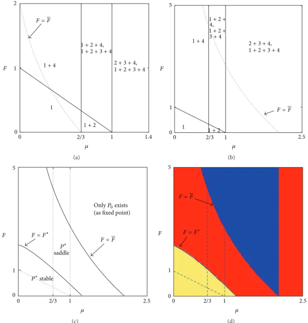
To the scope, we recall that, taking into account Remark 2,

the straight lines𝐹 = 1 − 𝜇 and 𝜇 = 1 − 𝛼/𝛽 induce us to

distinguish between regimes1 (i.e., 𝑈₁= R2₊),1 + 2 (i.e., both

𝑈₁and𝑈₂are involved), and, finally,1+4 (i.e., regions 𝑈₁and

𝑈₄must be considered).

On the other hand, it must be noticed that points(𝜇, 𝐹)

such that𝐹 > 1 − 𝜇 and 𝜇 > 1 − 𝛼/𝛽 represent parameter

values at which regimes1 + 2 + 4 or 2 + 3 + 4 or, finally, 1+2+

3+ 4, may emerge. These last open cases may be distinguished.

In fact, taking into account the proof of Lemma 1, if𝜇 < 1

(resp.,𝜇 > 1) then regimes 1 + 2 + 4 or 1 + 2 + 3 + 4 (resp.,

regimes2 + 3 + 4 or 1 + 2 + 3 + 4) can be present so that when

the straight line𝜇 = 1 is crossed, a change between regimes

may occur (see Figures 2(a) and 2(b)).

We also recall that, as it has been proved in Proposition 3,

points above the curve𝐹 = 𝛼𝛿/(𝜇𝛽 + 𝛼) − 𝜇 = 𝐹 are such that

only the extinction equilibrium exists as fixed point. Hence, if such a curve intersects the region characterized only by

regime1 given by set 𝑆 = {(𝜇, 𝐹) : 𝜇 > 0, 𝐹 > 0, 𝜇 + 𝐹 <

(9)

0 2/3 1 1.4 0 1 2 F 1 F = F 1 + 4 1 + 2 + 4, 1 + 2 + 3 + 4 2 + 3 + 4, 1 + 2 + 3 + 4 𝜇 1 + 2 (a) 0 2/3 1 2.5 0 1 5 F 1 F = F 1 + 4 1 + 2 + 4, 2 + 3 + 4, 1 + 2 + 3 + 4 1 + 2 + 3 + 4 1 + 2 𝜇 (b) 0 1 5 F F = F 0 2/3 1 2.5 𝜇 F = F∗ P∗stable P∗ saddle Only P0exists

(as fixed point)

(c) 0 2/3 1 2.5 0 1 5 F F = F 𝜇 F = F∗ (d)

Figure 2: Regions in the parameter plane(𝜇, 𝐹) related to the different regimes involved in the definition of system 𝑇 for 𝛼 = 20 and 𝛽 = 60. In (a)𝛿 = 2 while in (b) 𝛿 = 14.6. The black curves separate regions in which 𝑇 is defined by 𝑈₁(1),𝑈₁and𝑈₂(1 + 2),𝑈₁and𝑈₄(1 + 4), and so on. (c) Given the parameters as in (b), the bifurcation curves𝐹 = 𝐹∗and𝐹 = 𝐹 are depicted: they represent parameter values such that 𝑃∗_{loses its stability or the two fixed points merge, respectively. (d) For case (b) the regions denote different asymptotic dynamics for a given}

initial condition: in red is the 2-period cycle, in blue is the convergence to𝑃₀, and in yellow is the convergence to𝑃∗.

such that Proposition 4 applies; that is,𝑃₀is globally stable.

Such a region is given by𝑅₀ = {(𝜇, 𝐹) ∈ 𝑆 : 𝐹 > 𝐹} where

𝑅₀is not empty iff at the point(1 − 𝛼/𝛽, 𝛼/𝛽) the inequality

𝐹 > 𝛼𝛿/(𝜇𝛽 + 𝛼) − 𝜇 is satisfied, thus reaching the condition 𝛿 < 𝛽/𝛼, which holds, for instance, if 𝛿 is not too high (this case is presented in Figure 2(a)).

Taking into account the different regimes that may be

involved by𝑇 and Lemma 8, it can be noticed that if 𝜇 > 1 and

𝐹 > 𝐹, then 𝑈₃is not empty and consequently, as it has been

previously underlined, all initial conditions(𝑥(0), 𝑦(0)) ∈ 𝑈₃

are mapped into𝑃₀in one step.

Furthermore, recall that in Proposition 5 it has been

proved that if𝜇 < 1 and 𝛽 < 𝛽₁, then 𝑃∗ is locally stable

as long as𝐹 is small enough; that is, 𝐹 < 𝐹∗. The curve

𝐹 = 𝐹∗ _{is depicted in Figure 2(c) and it can be easily}

observed that if(𝜇, 𝐹) ∈ 𝐼((0, 0), 𝑟), then such conditions

hold, providing that if the capture mortality rate and the natural death rate are sufficiently low, then the coexistence

equilibrium is locally stable. In addition, since 𝐼((0, 0), 𝑟)

belongs to regime 1, then the map is smooth and defined

by 𝑇₁ in the whole plane R2₊ for all (𝜇, 𝐹) ∈ 𝐼((0, 0), 𝑟).

Since Proposition 6 applies, then no diverging trajectories are

produced by system𝑇, and consequently 𝑃∗ attracts all

tra-jectories starting from initial conditions different from(0, 0).

In Figure 2(c) the curves𝐹 = 𝐹 and 𝐹 = 𝐹∗ are depicted.

(10)

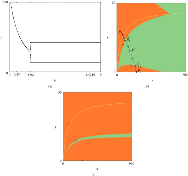
0 0.37 1.1282 4.4219 5 0 600 F x (a) 0 900 0 30 y x P∗ P2 P1 P2󳰀 P1󳰀 (b) 0 900 0 30 y x (c)

Figure 3: (a) One-dimensional bifurcation diagram for𝜇 = 0.63 and 𝛿 = 14.6: for a given initial condition the system converges to 𝑃∗or to𝐶₂as𝐹 is increased. (b) 𝐹 = 1.1. Before the flip bifurcation at 𝐹 ≃ 1.1282, 𝑃∗(white point) is locally stable and it coexists with a stable 2-period cycle (black points): their basins are depicted in green and orange, respectively. (c)𝐹 = 1.128. Immediately before the flip bifurcation the two coexisting attractors are depicted together with their own basins.

below𝐹 = 𝐹; that is, 𝑃∗ firstly loses its stability and then

merges.

In Figure 2(d), for each parameter’s combination, the blue

region represents convergence to𝑃₀, the red region represents

convergence to a2-period cycle, and, finally, the yellow region

represents convergence to𝑃∗. It is worth to observe that such

a picture has been obtained for an initial condition close

to𝑃∗, when it exists, or to the origin but inside region𝑈₁,

otherwise, and consequently it does not capture the possible coexistence of attractors which may occur in this kind of

models. Hence, an arising question is if𝑇 admits another

coexisting attractor, that is, if multistability emerges. In order to investigate this phenomenon, we present some numerical experiments in which we fix the value of the

natural mortality rate𝜇 and let the capture mortality rate

𝐹 vary. In particular, we focus on the following cases: 1. P.

mariae and 2. P. magdalenae.

Case 1 (P. mariae (𝜇 = 0.63)). Taking into account

Figure 2(d), it can be observed that if we fix𝜇 = 0.63 as

calculated for fish P. mariae, then the corresponding one-dimensional bifurcation diagram with respect to parameter 𝐹 is depicted in Figure 3(a); such a diagram illustrates the transition from a stable fixed point to a stable 2-cycle in a subcritical smooth flip bifurcation. Such a figure has been

depicted for an initial condition close to𝑃∗, when it exists, or

for(𝑥(0), 𝑦(0)) ∈ 𝐼(0, 𝑟) ∩ 𝑈₁if𝑃∗does not exist. In this last

case, it has been numerically verified that the same diagram

emerges for an initial condition(𝑥(0), 𝑦(0)) ∈ 𝐼(0, 𝑟) ∩ 𝑈₄.

This evidence enables us to conclude that if 𝜇 < 1 − 𝛼/𝛽

and being the parameter values fixed at the levels estimated for fish P. mariae, then the coexistence equilibrium is locally

stable as long as𝐹 < 𝐹∗ ≃ 1.1282 as proved in Proposition 5,

while if𝐹 > 1.1282, a stable 2-period cycle 𝐶₂ = {𝑃₁, 𝑃₂} is

(11)

However, even if at𝐹 = 𝐹∗the coexistence equilibrium loses stability via flip bifurcation, anyway the two period cycle

𝐶₂has been created when𝑃∗is still attracting, as it can be

observed in Figure 3(b) in which𝐹 = 1.1 < 𝐹∗ has been

considered. In fact the two-period cycle𝐶₂evidenced by two

black dots has been created by border collision in pair with

saddle 2-period cycle at𝐹 = 𝐹_BCB ≃ 1.08 (see, e.g., Radi et

al. [21], Gardini et al. [22], and Sushko et al. [19] for further details). As a consequence it can be observed that a border

collision bifurcation (BCB) saddle node occurs at𝐹 = 𝐹_BCB<

𝐹∗at which two period cycles are created, an attracting

2-period cycle𝐶₂and a saddle one𝐶󸀠₂ = {𝑃₁󸀠, 𝑃₂󸀠}. The interior

fixed point𝑃∗is still stable (white point) and it coexists with

the stable 2-period cycle𝐶₂(black points) while𝐶󸀠₂belongs

to the border separating the basin of attraction of𝑃∗and𝐶₂,

respectively.

If𝐹 is further increased approaching 𝐹∗, the two portions

of basins approach each other as in Figure 3(c) which is depicted immediately before the flip bifurcation: the saddle

2-period cycle𝐶󸀠₂ approaches 𝑃∗ and merges with it in a

subcritical flip bifurcation occurring at𝐹 = 𝐹∗ after which

the unique attractor is𝐶₂while𝑃∗is a saddle.

The region of bistability, that is, the region where the stable fixed point coexists with a stable 2-cycle (see Figures 3(b) and 3(c)), is bounded by the subcritical flip and border collision fold bifurcation points. When crossing these bound-aries the system displays hysteretic transitions from the stable fixed point to a stable 2-cycle and vice versa.

Comparing the bifurcations occurring in smooth systems with the BCB just described, we remark that the dynamic effects can be similar. However, a smooth bifurcation can be locally detected via the eigenvalues of the cycles. Thus, the occurrence of a smooth bifurcation can be found using econometric methods. In contrast, the occurrence of a border collision bifurcation can no longer be predicted via the eigenvalues of the cycles. In that sense, its occurrence is more dangerous, more unexpected. However, the role played by the eigenvalue in a smooth system is now replaced by the borders of the regions.

It is of interest to observe that𝐶₂continues to be locally

stable also if 𝐹 > 𝐹 = 4.4219, that is, if the coexistence

equilibrium has disappeared. Finally, notice that the2-period

cycle coordinates do not depend on the𝐹 value. Observe that

in the situation just presented only regimes1 and 1 + 4 are

involved. In the biological and fishery context this result is of great relevance especially for the case of P. mariae, because

it can be interpreted so that when fish mortality is 𝐹 >

𝐹 = 4.4219 and the coexistence equilibrium has disappeared, then the size of both subpopulations approximates to one of the two population sizes corresponding to the 2-period cycle, ensuring the conservation of the species. Furthermore, although mortality by fishing is very large, the species does not evolve towards extinction, but rather it is preserved since the 2-period cycle remains the unique attractor.

Case 2 (P. magdalenae (𝜇 = 0.897)). A similar situation

occurs if we consider fish P. magdalenae. In Figure 4(a) if𝐹 =

0.5 then an attracting 2-period cycle created by a saddle-node BCB coexists with the stable coexistence equilibrium and

then the sequence is as in Case 1; that is, at𝐹 = 𝐹∗ ≃ 0.6441

a subcritical flip bifurcation occurs, 𝑃∗ loses its stability,

and the 2-period cycle remains stable. In Figure 4(b) the situation occurring immediately before the flip bifurcation is presented.

Anyway, different from Case 1, a further scenario can

be described. At 𝐹 = 𝐹 ≃ 3.0586, 𝑃∗ merges; when

𝐹 crosses 𝐹, 𝐶₂ is still the unique attractor while regime

1 + 2 + 4 is presented (see Figure 1(d)). Anyway, if 𝐹 still

increases, then the region𝑈₃ will appear, which represents

the stable set of𝑃₀ which is a Milnor attractor. Hence, as it

is shown in Figure 4(c), a situation in which the attractor

𝐶2 and the Milnor attractor 𝑃0 coexist may emerge. The

blue region represents initial conditions that are mapped

into𝑃₀, while the points depicted in orange are the initial

conditions producing trajectories converging to the2-period

cycle. Notice that the two sets are separated by the white and the yellow curves depicted in panel (c), which represent

curves𝑓(𝑥, 𝑦) = 0 and 𝑔(𝑥, 𝑦) = 0, respectively.

In this case, an interesting question arising is related to the definition of a policy able to move the initial state from

the stable set of𝑃₀ to the basin of𝐶₂ in order to avoid the

extinction of the species. For instance, a policy which plans to stop fishing activity for a period may produce the effect of an increase in the size of both populations, so that, finally, the conservation of the species can be preserved in one of the two population sizes corresponding to the 2-period cycle. Finally notice that the situation just described cannot occur in Case

1 (P. mariae) since, according to part (ii) of Lemma 1, set𝑈₃

is empty for all𝐹.

The phenomenon of multistability plays an important role in the study of the evolution of dynamic models. Actually, if several attractors coexist, each of which with its own basin of attraction, the selected long-term state becomes path depen-dent and the structure of the basins of different attractors becomes crucial for predicting the long-term evolution of the system. Furthermore, an interesting question concerning policies aiming at forcing a given asymptotic state arises. For instance, in the situation presented in Figure 3(b), if at the initial state one of the subpopulations is very low, then the

system will converge to a2-period cycle. However, a policy

planning to stop fishing activity for a period may produce the effect of an increase in the size of both subpopulations, so that, finally, the equilibrium that will be approached can be the coexistence equilibrium. In a similar way, a policy may be conducted to move the initial condition from a point in the blue region to a point in the orange region of Figure 3(c) in order to avoid the extinction of the species.

5. Conclusions and Further Developments

The discrete time model proposed for a population of two-stage with recruitment and capture constitutes a new approach in order to understand the dynamics of some species with these characteristics which are exploited by humans, for example, fish species such as P. mariae and

P. magdalenae. Therefore, from the results reached, several

(12)

0 900 0 30 y x (a) 0 900 0 30 y x (b) 0 100 0 1 y x (c)

Figure 4: (a)𝐹 = 0.5. Before the flip bifurcation at 𝐹 ≃ 0.6441, 𝑃∗(white point) is locally stable and it coexists with a stable 2-period cycle (black points): their basins are depicted in green and orange, respectively. (b)𝐹 = 0.64. Immediately before the flip bifurcation the two coexisting attractors are depicted together with their own basins. (c)𝐹 = 60. A generic trajectory may converge to the extinction equilibrium 𝑃₀or to𝐶₂. The stable set of𝑃₀is depicted in blue while the basin of attraction of𝐶₂is depicted in orange.

the formulation of policies for the control of the capture and sustainability of the species modeled.

By using an analytical approach combined with numer-ical techniques, we distinguish between changes in the dynamics of the system due to the usual behaviors occurring in smooth maps and changes due to the presence of nonneg-ativity constraints. Considering the key role of the natural mortality and capture mortality rates, the study focuses on the role played by these parameters, while fixing the other parameters of the model at suitable levels.

An important result is that the system admits an attractor under certain conditions of the parameters. This result allows us to reach conditions such that the extinction equilibrium is globally stable. From a biological and fishery point of view,

this result is really relevant because it determines parametric conditions on capture that would make the species evolve towards its extinction, for any initial condition. Therefore, a fishery policy that controls capture effort and fishing methods can be adopted to prevent the species from being endangered. Moreover, another interesting result is that the system can undergo a border collision bifurcation in which the coexistence equilibrium, which is locally stable, coexists with a locally stable 2-period cycle. Its occurrence cannot be predicted via the eigenvalues of the cycles. In that sense, it is more dangerous, more unexpected, with respect to smooth bifurcations.

On the other hand, multistability plays an important role in the study of the evolution of the dynamical system. In

(13)

fact, if several attractors coexist, each of which with its own basin of attraction, the long-term evolution of the system will depend basically on the initial condition. In this respect, interesting questions about the policies aiming at forcing a given asymptotic state arise. For instance, a policy which plans to stop fishing activity for a period may produce an effect on the initial condition of both subpopulations, so that, finally, the population will approach the coexistence equilibrium, if it is locally stable, or to the 2-period cycle, with the purpose to conserve species over time and to avoid extinction.

Taking into account that the model developed in this work corresponds to a generalization of the discrete time version of the model Ladino et al. [12], it is of interest to compare the results of both studies. In particular, since we considered the real data, our study aims to demonstrate that when real cases are taken into account, richer dynamics can be exhibited, such as periodic fluctuations and multistability. Those phenomena cannot be found in Ladino et al. [12].

As a further step in this study more appropriate formu-lations of the discrete time model for a two-stage species with recruitment and capture can be taken into account. For instance, we plan to construct the discrete time framework starting from the equations and rules governing the dynamics of exploited populations while assuming that a given fixed time is required to pass from a state to the following one.

Competing Interests

The authors declare that they have no competing interests.

Acknowledgments

The authors gratefully acknowledge that this work has been performed within the activity of the Collegio Matteo Ricci

2013 Project, financed by the University of Macerata, Italy,

and the Services Commission awarded by University of Los Llanos, Colombia, by Superior Resolution 065 of 2014. Jose C. Valverde was also supported by the Ministry of Economy and Competitiveness of Spain under Grant MTM2014-51891-P and by the FEDER OMTM2014-51891-P2014-2020 of Castilla-La Mancha under Grant GI20163581.

References

[1] Y. A. Kuznetsov, Elements of Applied Bifurcation Theory, Springer, New York, NY, USA, 2004.

[2] F. Balibrea, A. Martinez, and J. C. Valverde, “Local bifurcations of continuous dynamical systems under higher order condi-tions,” Applied Mathematics Letters, vol. 23, no. 3, pp. 230–234, 2010.

[3] R. Yuan, W. Jiang, and Y. Wang, “Saddle-node-Hopf bifurcation in a modified Leslie-Gower predator-prey model with time-delay and prey harvesting,” Journal of Mathematical Analysis

and Applications, vol. 422, no. 2, pp. 1072–1090, 2015.

[4] D. Franco and J. Per´an, “Stabilization of population dynamics via threshold harvesting strategies,” Ecological Complexity, vol. 14, pp. 85–94, 2013.

[5] D. J. W. Simpson, Bifurcations in Piecewise-Smooth Continuous

Systems, vol. 70 of Nonlinear Science Series A, World Scientific,

New Jersey, NJ, USA, 2010.

[6] M. I. Feigin, “Doubling of the oscillation period with C-bifurcations in piecewise continuous systems,” Journal of

Applied Mathematics and Mechanics (PMM), vol. 34, pp. 861–

869, 1970.

[7] M. Di Bernardo, M. I. Feigin, S. J. Hogan, and M. E. Homer, “Local analysis of C-bifurcations in ndimensional piecewise-smooth dynamical systems,” Chaos, Solitons and Fractals, vol. 10, no. 11, pp. 1881–1908, 1999.

[8] H. E. Nusse and J. A. Yorke, “Border-collision bifurcations including ‘period two to period three’ for piecewise smooth systems,” Physica D: Nonlinear Phenomena, vol. 57, no. 1-2, pp. 39–57, 1992.

[9] S. Brianzoni, E. Michetti, and I. Sushko, “Border collision bifur-cations of superstable cycles in a one-dimensional piecewise smooth map,” Mathematics and Computers in Simulation, vol. 81, no. 1, pp. 52–61, 2010.

[10] D. J. Simpson and J. D. Meiss, “Aspects of bifurcation theory for piecewise-smooth, continuous systems,” Physica D: Nonlinear

Phenomena, vol. 241, no. 22, pp. 1861–1868, 2012.

[11] A. Agliari, P. Commendatore, I. Foroni, and I. Kubin, “Border collision bifurcations in a footloose capital model with first

nature firms,” Computational Economics, vol. 38, no. 3, pp. 349–

366, 2011.

[12] L. M. Ladino, C. Mammana, E. Michetti, and J. C. Valverde, “Discrete time population dynamics of a two-stage species with recruitment and capture,” Chaos, Solitons & Fractals, vol. 85, pp. 143–150, 2015.

[13] L. M. Ladino and J. C. Valverde, “Population dynamics of a two-stage species with recruitment,” Mathematical Methods in the

Applied Sciences, vol. 36, no. 6, pp. 722–729, 2013.

[14] CCI and INCODER, Pesca y Acuicultura Colombia 2006, Coor-poraci´on Colombiana Internacional CCI. Instituto Colombiano de Desarrollo Rural INCODER, Bogot´a, Colombia, 2006. [15] I. Kubin and L. Gardini, “Border collision bifurcations in boom

and bust cycles,” Journal of Evolutionary Economics, vol. 23, no. 4, pp. 811–829, 2013.

[16] S. Banerjee and C. Grebogi, “Border collision bifurcations in two-dimensional piecewise smooth maps,” Physical Review E, vol. 59, no. 4, pp. 4052–4061, 1999.

[17] D. J. Simpson, “On the relative coexistence of fixed points and period-two solutions near border-collision bifurcations,”

Applied Mathematics Letters, vol. 38, pp. 162–167, 2014.

[18] H. E. Nusse and J. A. Yorke, “Border-collision bifurcations for piecewise smooth one-dimensional maps,” International

Journal of Bifurcation and Chaos, vol. 5, no. 1, pp. 189–207, 1995.

[19] I. Sushko, L. Gardini, and T. Puu, “Regular and chaotic growth in a Hicksian floor/ceiling model,” Journal of Economic Behavior

and Organization, vol. 75, no. 1, pp. 77–94, 2010.

[20] A. Medio and M. Lines, Nonlinear Dynamics: A Primer, Cam-bridge University Press, CamCam-bridge, UK, 2001.

[21] D. Radi, L. Gardini, and V. Avrutin, “The role of constraints in a segregation model: the symmetric case,” Chaos, Solitons &

Fractals, vol. 66, pp. 103–119, 2014.

[22] L. Gardini, D. Fournier-Prunaret, and P. Charg´eP, “Border collision bifurcations in a two-dimensional piecewise smooth map from a simple switching circuit,” Chaos, vol. 21, no. 2, Article ID 023106, 2011.

(14)

Submit your manuscripts at

http://www.hindawi.com

Hindawi Publishing Corporation

http://www.hindawi.com Volume 2014

Mathematics

Journal of

http://www.hindawi.com Volume 2014 Mathematical Problems in Engineering

Hindawi Publishing Corporation http://www.hindawi.com

Differential Equations International Journal of

Volume 2014

http://www.hindawi.com Volume 2014 Hindawi Publishing Corporationhttp://www.hindawi.com Volume 2014

Mathematical PhysicsAdvances in

Complex Analysis

Journal of

Optimization

Journal of

Combinatorics

http://www.hindawi.com Volume 2014 International Journal of

Journal of

Function Spaces

Abstract and Applied Analysis Hindawi Publishing Corporation

http://www.hindawi.com Volume 2014 International Journal of Mathematics and Mathematical Sciences

Hindawi Publishing Corporation http://www.hindawi.com Volume 2014

The Scientific

World Journal

Discrete Dynamics in Nature and Society

Discrete Mathematics

Journal of

http://www.hindawi.com Volume 2014 Hindawi Publishing Corporationhttp://www.hindawi.com Volume 2014

Border Collision Bifurcations in a Generalized Model of Population Dynamics

Research Article