Amplification and displacement of chaotic attractors by means of unidirectional chaotic driving

Amplification and displacement of chaotic attractors by means of unidirectional chaotic driving

J. M. Gonza´lez-Miranda

Departamento de Fı´sica Fundamental, Universidad de Barcelona, Avenida Diagonal 647, 08028 Barcelona, Spain ~Received 18 November 1997; revised manuscript received 26 January 1998!

Chaotic systems, when used to drive copies of themselves~or parts of themselves! may induce interesting behaviors in the driven system. In case the later exhibits invariance under amplification or translation, they may show amplification~reduction!, or displacement of the attractor. It is shown how the behavior to be obtained is implied by the symmetries involved. Two explicit examples are studied to show how these phenomena mani-fest themselves under perfect and imperfect coupling.@S1063-651X~98!13206-3#

PACS number~s!: 05.45.1b, 42.65.Sf, 47.52.1j, 95.10.Fh

Pecora and Carroll @1# have reported a driving method ~PCM for short! that allows synchronization between two identical chaotic systems. This has been successfully imple-mented in experiments; in particular, it has been observed in electric circuits,@2,3# and used in telecommunication devices @4#. Further developments have focused towards generalized forms of synchronization @5,6#, understood as situations where the two systems evolve in perfect correlation despite that their distance in phase space does not go to zero, as in the Pecora and Carroll synchronization. Recently, there have appeared two interesting behaviors of a response under cha-otic driving @7#: the amplification ~reduction! of a chaotic attractor, and the sustained evolution of the driven system, repeating the drive attractor, in a region of phase space far from where the stable attractor lies. Because the driving scheme proposed is the same as that used by Pecora and Carroll for synchronization, there is no doubt about the pos-sibility of preparing an experimental setting for their obser-vation. Moreover, such driving situations might occur in na-ture~e.g., the case of neuronal systems has been the object of speculation @1,8#!. The possibilities of getting amplified ~shrunken! copies of a given chaotic signal, or copies of a system steadily evolving within variable ranges different from those imposed by its constrains, enriches the range of behaviors expected from driven chaotic systems, and then provides new tools for prediction, explanation, or application in science and technology. The aims of this report are to show how the behavior to be obtained is implied by the system symmetries, to study these systems to gain insight into how these phenomena manifest themselves, and to show that they are robust enough to be observed in experiments.

Consider a dissipative nonlinear dynamical system

dx

dt5f~x!, ~1!

with xPRn, whose evolution is chaotic and occurs in a strange attractor, A @9#. Divide the set of x coordinates in two subsets x1PRn1 and x2PRn2, where n11n25n, such that the latter is invariant under a set of transformations of coordinates, T_P, that act only on the variables, x₂. Then, the dynamical equations are rewritten as

dx1

dt 5f1~x1,x2!, ~2a!

dx2

dt 5f2~x1,x2!, ~2b! In particular, given this decomposition, the x2subsystem will be attracted to a set of pointsA2,Rn2.

The set of transformations of coordinates TP:x2→x2*, fromRn_2→Rn_{2, all have the same functional form, each} par-ticular transformation is specified by the values of a set of parameters P5(P₁, P₂, . . . , P_q), which change continu-ously in a given interval, PiP@ai,bi#,R, such that 0

P@ai,bi#, to produce the different transformations of the set. It is assumed that these transformations are continuous in the sense thatuP2P

8

u→0 implies uTP(x2)2TP8(x2)u→0 for all points x₂PA₂. Moreover, T_P→I, when P→0, where I is the identity. Under any one of this transformations Eq. ~2b! re-mains unchanged; i.e., Eq. ~2b! holds for x₂* as well as for

x2. Two particular transformations of that type will be stud-ied: an amplitude transformation, defined by T_A(x₂)[A•x₂, with APR, and a displacement transformation, defined by TD(x2)[x21D, with DPRn2.

In the PCM @1,8#, for that type of system, the drive is described by Eqs. ~2!, and a copy of the symmetric sub-system x2, denoted by x2

8

, called the response, is prepared so that its dynamics is governed by the equation

dx₂

8

dt 5f2~x1,x2

8

!, ~3! which is driven by the variables x1, that constitute the drive signal. The trajectory x₂

8

(t)5x2(t) is a solution of Eq.~3! if

x2(t) is a solution of Eqs.~2! in A2. However, for this syn-chronized state to be asymptotically stable, all Lyapunov ex-ponents of the response, called conditional Lyapunov expo-nents, have to be negative. Synchronization can be tested by computing the largest conditional Lyapunov exponent L, which can be obtained from the time evolution of the drive as L5 lim t→` 1 t ln udx2~t!u udx2~0!u , ~4!

wheredx₂[ux₂

8

2x₂u is an infinitesimal deviation of x₂

8

from

x₂. IfL,0, it is guaranteed that there will be asymptotically

PHYSICAL REVIEW E VOLUME 57, NUMBER 6 JUNE 1998

57

stable synchronization from an appropriate subset of initial conditions of drive and response@8,10#.

For the type of symmetric systems studied in this paper, when the coordinate transformation TP is applied to the x2 subsystem attractor, A2, one obtains a copy of it, TP(A2), which somehow mimics A2. For the amplitude transforma-tion TP(A2) is an enlarged or shrunken copy ofA2, while for the displacement transformation it is a fair copy of A2 dis-placed from the region where the stable attractor evolves. We know that when initial conditions of drive and response are such that x₂

8

(0)5x2(0) the evolution of x2 and x2

8

is such that x₂

8

(t)5x₂(t) for t.0. Therefore, because Eq. ~2b! holds for x₂*, it must happen that if the response initial condition is TP@x2(0)#, it will evolve in TP(A2) following a trajectory in perfect synchrony with x2(t) that follows some type of copy of A2, amplified~shrunken! or displaced.

For these systems, the largest conditional Lyapunov ex-ponent has to be zero. Because TP is continuous, a single

small perturbation applied to the response, when it is follow-ing a trajectory in T_P(A₂), will send it to another trajectory, in TP1dP(A2), similar and close to the former where it will stay. Because TP→I, when P→0, one can have the points of

TP(A2) as close as the point ofA2 as desired. Therefore, if the initial condition for the response is T0@x2

8

(0)#, i.e.,

x2

8

(0)5x2(0), it will follow a trajectory in T0(A2)5A2that exactly reproduces x2(t). Then, a small perturbation applied to the response evolving in A2will send it to a trajectory in T_dP(A2), withdP small, so that it is a close reproduction of the unperturbed trajectory inA2. Therefore, there is neither divergence,L.0, nor convergence, L,0, of close trajecto-ries, and then, L50.

In particular, for the case of the amplitude transformation, every initial condition of the response will evolve in a set, TA(A2), whose points are related to those of the original system attractor by means of x₂

8

5Ax2, with the value of A determined by the values of the initial condition. Therefore, dx2(t)5ux2

8

(t)2x2(t)u5uA21uux2(t)u, and with udx2(0)u .uA21uux2(0)u, with both x2(t) and x2(0) points inA2, it must be L5 lim t→` 1 tln uA21uux2~t!u udx2~0!u 50 ~5!

because the argument in the logarithm is a fluctuating bounded quantity. For the case of the displacement transfor-mation, every initial condition of the response will evolve in a set of points, TD(A2), which is related to the original sys-tem attractor by means of x₂

8

5x₂1D, with the value of D determined by the values of the initial condition. Therefore, dx2(t)5ux2

8

(t)2x2(t)u5uDu, and with udx2(0)u.uDu, it must be L5 lim t→` 1 tln uDu udx2~0!u50 ~6!

because the logarithm argument is a bounded constant. The existence of this non-negative conditional Lyapunov exponent means that, in the present case, we will not have asymptotically stable behaviors; i.e., ux₂

8

(t)2TP@x2(t)#u→0 forux₂

8

(0)2T_P@x₂(0)#u<d, as would occur ifL,0. Instead

we have what it is known as uniform stability@9#, which is defined by the following condition: if ux2

8

(0)2TP@x2(0)#u <d for some small positive real numberd, there must exist another small positive real number «, such that ux₂

8

(t) 2TP@x2(t)#u<« for t>0. It is to be noted that uniform sta-bility, although weaker then asymptotic stasta-bility, is stronger than another type of stability, frequently found in nature and technology, orbital stability. This is defined@9# as the case in which if ux₂

8

(0)2T_P@x₂(0)#u<d, there must exist an « and some function t*(t) such thatux₂

8

(t*)2TP@x2(t)#u<« for t >0; so, in this last case, there is no isochronous correspon-dence between the two time evolutions that one finds in the cases of asymptotic and uniform stability.

The amplitude transformation has been studied in the Lo-renz model~LM for short! for convection in fluids @11# given by x˙5s( y2x), y˙5(r2z)x2y, and z˙5xy2bz. The values of the parameters are s516, r545.92, and b54, as in @8#. The equations for x and y are invariant under an amplitude transformation TA(x, y )[(Ax,Ay). Therefore, one can ob-serve the amplification of the signal in the x-y plane. Then, the appropriate drive signal is z, and the response subsystem is described by

x˙

8

5s~y

8

2x

8

!, ~7a! y˙

8

5~r2z!x

8

2y

8

. ~7b! The displacement transformation is studied in the double scroll ~DS for short!, which is a model of an electric circuit @12,3#: x˙5a@y2x2 f (x)#, y˙5x2y1z, and z˙52by , where f (x)5bx112(a2b)@ux11u1ux21u#. The parameter values studied are a510, b514.87, a521.27, and b520.68 as in @3#. The equations for x and z are invariant under TD(z)[z1D; therefore, one may obtain a displace-ment of the attractor in the z direction using as the response a copy of the (x,z) subsystem. Then, the drive variable will be y and the response equations will be given by

x˙

8

5a@y2x

8

2 f~x

8

!#, ~8a!

z˙

8

52by . ~8b!

The numerical results presented have been obtained by means of numerical integrations of the above equations using a fourth-order Runge-Kutta algorithm with a time step of 0.003 for LM, and 0.02 for DS.

The conditional Lyapunov exponents have been obtained from the integration of the variational equation

d~dx₂!

dt 5Dw„h~x1,x2

8

!…dx2, ~9! where Dw„h(x1,x2)… is the Jacobian of the response at x2

8

5x2, where the time evolution of x1 and x2 is given by Eqs. ~2!. In Fig. 1~a!, for LM, and Fig. 1~b!, for DS, there appear some representative results for the parameter dependence of the conditional Lyapunov exponents for the response, and the Lyapunov exponents for the original three-dimensional system. These figures show that the largest conditional Lyapunov exponent, being determined by the symmetries of

the system, is null and does not change when the system parameters change, despite that this changes the behavior of the system.

To observe the amplification of the attractor, in LM, and the displacement, in DS, the appropriate equations of motion have been integrated in each case. The corresponding phe-nomena have been monitored by means of parametric plots of the variables of the response versus the variables of the drive, which appear as straight lines when both signals evolve in perfect synchrony. The amplification A is mea-sured by the slope of the straight line, and the displacement D by its ordinate in the origin. A case for LM with initial conditions such that the A.5 is displayed in Fig. 2~a!, which shows how the y

8

signal is an amplified copy, by a factor 5, of the y signal ~a plot for the x signal would have to look almost the same!. The results in Fig. 2~b!, for DS with initial conditions appropriate to obtain D.10, show how x

8

(t) 5x(t), while z

8

(t).z(t)110. Similar calculations per-formed for the same systems using different initial condi-tions resulted in the same types of behaviors, but with dif-ferent numerical values for A or D.

The magnitude of the amplification, or displacement, is determined by the initial conditions of the systems. Because of the uniform stability that characterizes this case, we have to expect a linear relation between A, or D, and the initial distance between the systems. To observe this dependence I have chosen a point in the stable attractor as a fixed initial condition for the drive, and studied the degree of amplifica-tion, or displacement, for initial conditions of the response evenly distributed on a rectangular grid in the x

8

-y

8

plane, for LM, or the x

8

-z

8

plane, for DS. For a given drive initial

condition, I obtained that, for LM, the functions A 5A(x0

8

, y0

8

) are given by two symmetric planes that intersect the A50 plane along a straight line that crosses the origin of coordinates. The inclination and orientation of these planes, given respectively by the angle u between the planes A 5A(x0

8

, y0

8

) and A50, and by the angle f between the straight line made by the intersection between those planes and the x₀

8

axis, change with the values of the drive initial condition. For DS, D5D(x₀

8

,z₀

8

) is given by a plane whose intersection with the D50 plane is a straight line parallel to the x₀

8

axis. The inclination and orientation of this plane does not change with the initial condition of the drive, while the distance between its intersection with the D50 plane and the x₀

8

axis, d, changes with the drive initial condition. To ex-plore those dependencies on drive initial conditions I have determined the functions A5A(x₀

8

, y₀

8

) and D5D(x₀

8

,z₀

8

) for sets of drive initial conditions made of points taken con-secutively along a trajectory in the stable attractor. Figure 3~a!, for A(x₀

8

,y₀

8

), and Fig. 3~b!, for D(x₀

8

,z₀

8

), show thatu and f, as well as d, change continuously and smoothly as the drive evolves in its attractor.

To study the behavior of the response trajectories in the presence of external noise, a series of time evolutions have been performed adding a Gaussian white noisedtto the drive signal. The control parameter in this study is the dispersion in the distribution ofdt,s, given in units of the amplitude of the signal considered. Calculations made for a fixed obser-vational time window of 104 _{time steps ~about 100 orbits!} showed that, once the time window is fixed, there is a level of noise below which one obtains a response trajectory that accurately reproduces the drive attractor amplified ~shrunken!, for LM, or displaced, for DS. Once that level of noise is overcome these trajectories exhibit a diffusivelike behavior: for LM one obtains amplified copies of the drive attractor with an amplitude that fluctuates, and for DS one

FIG. 1. Lyapunov exponents ~thin lines! and conditional Lyapunov exponents~thick lines! as functions of the parameters of the system:~a! r dependence for LM, and ~b!b dependence for DS.

FIG. 2. Amplification and displacement monitored by means of parametric plots:~a! y signal for LM with initial conditions chosen to get A.5, and ~b! x and z signals for DS with initial conditions chosen to obtain D.110.

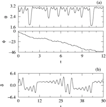
FIG. 3.~a! Time dependence of the angles,u and f, for LM. ~b! The same for the distancedfor DS.

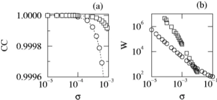
obtains displaced reproductions of the drive that shift up and down along the z axis. Moreover, I have studied the average size of the window, W, in which the response reproduction of the attractor is acceptable, as a function of the amplitude of the noise. The quantity W was defined as the average length of the time interval in which a fit to a straight line of x

8

5x

8

(x) and y

8

5y

8

(y ) ~for LM!, or x

8

5x

8

(x) and z

8

5z

8

(z) ~for DS! starts to fail for each level of noise. Such a breakdown of the fit was defined as the case when the cor-relation coefficient of the fit drops below 0.9999. This choice, although somewhat arbitrary, is based on results ob-tained for the dependence of this quantity with the level of noise for a fixed time window (104time steps! as those dis-played in Fig. 4~a!. The results obtained for W(sz) and W(sy), displayed in Fig. 4~b!, show that these functions are potential laws, and increase as the noise level decreases.

In conclusion, when chaotic systems that exhibit invari-ance properties under a special type of continuous transfor-mation are subject to chaotic driving under a PCM, they can undergo interesting synchronizationlike phenomena. These include partial amplification of the attractor, and displace-ment of it to a region of phase space where the original system is unstable. The particular orbit is determined by the initial conditions. It is a consequence of these symmetries that the largest conditional Lyapunov has to be null; then, the stability is not asymptotic, but uniform. The numerical study

of these phenomena has shown that under perfect coupling the largest conditional Lyapunov exponent is indeed null, it is possible to observe amplified or displaced trajectories in the computer simulations, and the degree of amplification or displacement obtained is smoothly dependent on the initial conditions. Computer simulations under situations of exter-nal noise have shown that the phenomena studied here can allow experimental observation.

This research was supported by DGICYT, through Project Nos. PB93-0780 and PB96-0392.

@1# L. M. Pecora and T. L. Carroll, Phys. Rev. Lett. 64, 821 ~1990!.

@2# T. L. Carroll and L. M. Pecora, IEEE Trans. Circuits Syst. 38,

453~1991!.

@3# L. O. Chua, L. Kocarev, K. Eckert, and M. Itoh, Int. J.

Bifur-cation Chaos Appl. Sci. Eng. 2, 705~1992!.

@4# K. M. Cuomo and A. V. Oppenheim, Phys. Rev. Lett. 71, 65 ~1993!.

@5# R. E. Amritkar and N. Gupte, Phys. Rev. A 44, R3403 ~1991!. @6# N. F. Rulkov, M. M. Sushchik, L. S. Tsimring, and H. D. I.

Abarbanel, Phys. Rev. E 51, 980~1995!.

@7# J. M. Gonza´lez-Miranda, Phys. Rev. E 53, R5 ~1996!. @8# L. M. Pecora and T. L. Carroll, Phys. Rev. A 44, 2374 ~1991!. @9# E. Atlee Jackson, Perspectives of Nonlinear Dynamics

~Cam-bridge University Press, New York, 1991!.

@10# P. Badola, S. S. Tambe, and B. Kulkarni, Phys. Rev. A 46,

6735~1992!.

@11# E. N. Lorenz, J. Atmos. Sci. 20, 130 ~1963!.

@12# T. Matsumoto, L. O. Chua, and M. Komuro, IEEE Trans.

Cir-cuits Syst. 32, 798~1985!.

FIG. 4.~a! Breakdown of the synchronizationlike behavior mea-sured by the correlation coefficient (CC) for LM~circles! and DS

~squares!. ~b! Window size where the response is a fair copy of the

drive attractor as a function of the amplitude of the noise for LM

~circles! and DS ~squares!.