UNIVERSITY
OF TRENTO
DIPARTIMENTO DI INGEGNERIA E SCIENZA DELL’INFORMAZIONE
38100 Povo – Trento (Italy), Via Sommarive 14
http://www.disi.unitn.it
Modeling a distributed Heterogeneous
Communication System using Parametric Timed
Automata
Thi Thieu Hoa Le, Luigi Palopoli, Roberto Passerone and Yusi Ramadian
April 2010
Technical Report Number: DISI-10-031
Modeling a distributed Heterogeneous Communication System
using Parametric Timed Automata
Thi Thieu Hoa Le, Luigi Palopoli, Roberto Passerone, Yusi Ramadian
Department of Information Engineering and Computer Science
University of Trento, Italy
[email protected]April 20, 2010
Abstract
In this report, we study the application of the Para-metric Timed Automata(PTA) tool to a concrete case of a distributed Heterogeneous Communication System (HCS). The description and requirements of HCS are presented and the system modeling is explained care-fully. The system models are developed in UPPAAL and validated by different test cases. Part of the sys-tem models are then converted into parametric timed automata and the schedulability checking is run to pro-duce the schedulability regions.
1
Introduction
Symbolically computing the region in the parameters space that guarantees a feasible schedule (given a set of real-time tasks characterised by a set of parameters and activation patterns) is a novel approach to the compu-tation of schedulability regions[2]. This method is of great usefulness, for example, once the feasible regions have been identified, the system designer can choose quickly a correct set of parameters that could make the system works properly. Moreover, he can also be as-sisted in optimizing the system performance while still keeping the system schedulable.
Parametric timed automata have been approached differently in the literature. In [7] given a real-time sys-tem and some sys-temporal formula which may contain pa-rameters, and a constraint over the papa-rameters, a model-checking problem is to verify whether every allowed parameter assignment could guarantee that the real-time system satisfies the formula. Instead, in [2] sensitivity constraints over the interested parameters are computed
and then joined together to produce the schedulability region of the system.
Another interesting work on PTA is studied in [8] where the authors use a prototype extension of UP-PAAL [4] for linear parametric model checking and show decidability results for the verification of L/U au-tomata. For this special class, the problem of deciding whether there exists a parameter valuation such that a given location s is reachable, is indeed decidable while it is not for the full class. The idea to this emptiness problem is then generalized in [2] in order to produce the parameter region in which the system is unschedu-lable.
In the context of asynchronous circuits, E. Andre et al. [9] propose a method of synthesizing constraints of a timed automaton, given an initial set of param-eter values for which the system is known to behave properly. The authors ensure that for any two valua-tions of parameters satisfying these constraints, the be-haviors of the timed automata are time-abstract equiva-lent. Although the method will terminate as long as all symbolic traces computed from a given reference pa-rameter valuation are either of finite length or trivially cyclic, it has been shown to be particularly suitable in the framework of asynchronous circuits. A. Cimatti et al.’s solution to the synthesis of constraints [2] is also symbolic but but differs from the former approach in many aspects. The later aims at symbolically comput-ing the region of parameter space that makes the system feasible by enumerating all possible traces that could drive the system into an error state and identifying, for each of them, the subsets of the parameter space that are compatible with the trace. In addition, the method does not make use of reference parameter valuations
and it is proved to converge for periodic task systems with bounded offsets.
In fact, the method in [2] can be applied widely in real-time systems adopting a fixed priority mechanism and in an effort to help with the development of the PTA prototype tool, we have tried to apply the tool to an in-dustrial embedded application. The application is first modeled in UPPAAL and validated by different ground sets of parameters. Part of the system models are then converted into parametric timed automata which are then analyzed by the PTA tool in order to produce the feasible region.
This report is organized as follows. Section 2 de-scribes the application and its requirements. In sec-tion 3, the UPPAAL models for the applicasec-tion are ex-plained in detail. These models are then validated by verifying different sets of parameters in section 4. Next, section 5 presents the parametric analysis after running the PTA tool. Finally, section 6 concludes the report and suggests future work.
2
HCS and Parametric Timed
Au-tomata
SensorSERVER CONTROL SCREEN
NAC WAP Sensor NAC NAC DEVICE DEVICE DEVICE DEVICE DEVICE DEVICE DEVICE
Figure 1: Heterogeneous Communication
Sys-tem(HCS)
The distributed Heterogeneous Communication System (HCS) contains various devices, wired and wireless communication networks and a common
server. The HCS provide control, monitoring and data processing of various subcomponents through heteroge-neous networks. The server is connected to different de-vices such as sensors and actuators via wired and wire-less protocols. The various devices are connected to the server through Network Access Controllers (NAC). The architecture of the HCS is described in more detail in [1].
HCS provides two important applications that can be deployed on end devices. One is to transmit audio data periodically to end devices every audPeriod ms from the server. The other application is to synchronize clocks using the Precision Time Protocol (PTP, IEEE1588[5]). A general HCS is depicted in figure 1, based on wired and wireless components. The HCS system consists of the following components: SERVER, DEVICE, NACs, wired and wireless networks. The HCS server is con-nected to all NACs in a daisy-chain topology. The NACs perform the gateway function between the back-bone and the end devices. Wireless devices are accessed via wireless access point (WAPs), and WAPs are con-nected directly to NACs. Functions of the WAPs are similar to the NACs functions, in particular synchro-nization with the network and server, data routing be-tween NACs and wireless network.
SERVER
MEDIUM
DEVICE
packet_out packet_in
play
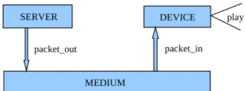
Figure 2: General schema of audio streaming over a network
Figure 2 illustrates a common design approach for audio streaming. More detail can be found in [1]. Such a stream of the HCS has a number of noticeable charac-teristics as follows:
• The communication between the server and device
is asynchronous.
• The server sends an audio packet every
audP eriod ms.
• An audio packet is characterized by two parame-ters: a sequence numberi and a timestamp ti
de-noting the time the packet has to be played at the device.
• Packets arrive at the device (except they get lost)
with a minimal latency Lmdm = Lmin and a
maximal latencyLmdm = Lmax
• The NACs simply forward the incoming packets
to the devices. And packets passing through the NACs have to experience a further delay ofLnac
ms during which they are preprocessed by the NACs.
• When a packet is received by the device, it needs τ ms to process the packet after which it is ready
to receive the next packet.
• The medium is unreliable, it may lose and reorder packets.
Figure 3: Time sequence diagram of message
ex-changed between master and slave clock to achieve time synchronization
Figure 3 depicts the clock synchronization of the slave clock with the master clock based on PTP. Ev-ery component of HCS has a local clock and PTP runs in the server, devices and NACs. Various timing delays are to be guaranteed, for example, in a scenario where two devices are connected to the server both wired and wireless, it should be guaranteed that both devices are synchronized within an error of 0.1ms (synchronization precision).
The ideal objective is to identify the parameter space-the largest region in which space-the correct functioning of au-dio streaming and clock synchronization can be guaran-teed by using the novel method proposed in [2]. One re-quirement regarding the correct functioning of the audio
application, for instance, could be the maximal time dif-ference between sending an audio packet and playback of the audio packet at the devices is less than 0.1ms. Another synchronization requirement could be to en-sure the synchronization precision is bounded by 0.1ms, given different timings on wired and wireless network.
However, HCS is too complex to be parametrically-modeled completely. Therefore, before applying the parametric timed automata (PTA) approach, we need to relax some of the above requirements. The simpli-fied system would contain only one server and many NACs and devices where one NAC may be associated to at most one device and one other NAC. Also, for the time being we would just focus on modelling the PTP part on the server and devices. Additionally, ev-ery audio packet will have to experience a maximal
de-lay when traversing through the medium (Lmdm =
Lmax). Furthermore, the last two characteristics of
the HCS audio streaming and the timing PTP delay are temporarily not considered and would be in the fu-ture as the next modelling step. Lastly, assuming that the transmission priority of the packets is as follows:
P riorSync > P riorF ollow U p > P riorDelay Res >
P riorDelay Req > P riorAudio. The system high level
description can be viewed logically as in figure 4(a) or figure 4(b).
(a)
(b)
3
UPPAAL Models
The models of HCS are first developed in UPPAAL[4] because UPPAAL allows graphically-modeling ability which assists model-developers in de-bugging and testing their models.
3.1
Integer clock
In UPPAAL, HCS is modeled as a network of ex-tended timed automata with global real-valued clocks and integer variables. Since the clock value is neces-sary in the PTP protocol, we need to retrieve the clock value which is impossible in UPPAAL as it does not support real variables as well as clock value retrieval. And integer clocks are invented to overcome this hur-dle. In fact, an integer clock is an integer variable re-turning the integer part of a real-valued clock. This ap-plies to real clocks which have no clock drift. How-ever, since the local clocks in the server and devices usually drift compared to the actual time, we need to adjust the operation of integer clocks in order to re-trieve the clock value within a certain precision. As-suming we have a clock drifte (0 < e), a real clock c and an integer clock ci. Actually, e should be a real
variable but as this is not allowed in UPPAAL, e has
to be integerized. That is, if we want to take care of up to n digits after the decimal point, we multiply e
and10n together. For example withn = 2, e = 95
means the drift of 0.95 andc = 0.95 ∗ t where t is
not a drifting clock. Thus, ci increases by 1 when t = 100/e = 100/95 = 1.052631579. Again,
UP-PAAL does not allow comparisons of clocks with real values, so we have to integerize100/e and make it even
more precise by multiplying it by some precisionprec.
With a three-digit precisionprec = 1000, for instance, ci increases when t = 1000 ∗ 100/95 = 1052, that is
we are scaling the bound at which the integer clock is changed. Henceci is more precise. Furthermore, every
integer variable will finally overflow if it keeps increas-ing, therefore to ensure the correctness of the whole sys-tem, it is necessary to reset integer clocks to 0 whenever they reach a predefined clock limitclkLimit.
3.2
Server
The server is modeled as a network of five timed au-tomata, one of which models the server integer clock, two of which model the PTP protocol running in the
server and the others model the audio sending and buffering operations of the server.
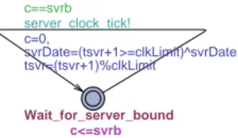
Wait_for_server_bound c<=svrb c==svrb server_clock_tick! c=0, svrDate=(tsvr+1>=clkLimit)^svrDate, tsvr=(tsvr+1)%clkLimit
Figure 5: The server integer clock
The timed automaton modeling the server integer clock is shown in figure 5. At the beginning the clock bound of the server issvrb = prec ∗ 100/esvr where prec is the digit precision and esvr is the server clock
drift. When clockc reaches the bound, the server
in-teger clock tsvr will increase by 1 and c is reset to
0. As said above, to prevent the overflow situation, when tsvr reaches the clock limit clkLimit, it will
be reset to 0. Because the server integer clock is re-set everyclkLimit time units and so is the device
inte-ger clock, it is crucial to distinguish the states of two clocks, that is whether they have been reset or not. Given that the difference of the two clocks can never exceed clkLimit, we invent the notion of ”odd date”
and ”even date”. The clocks at the beginning show the time in ”even date” and when they reach the clock limit, the displayed dates are changed to ”odd date” and vice versa. The server date is encoded in the variable
svrDate which results from the binary operation XOR: svrDate = (tsvr + 1 >= clkLimit) XOR svrDate.
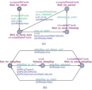
The PTP timed automata are depicted in figure 6. Figure 6(a) illustrates the first two steps of the synchro-nization procedure shown in figure 3 and figure 6(b) de-scribes the last step. In the figures, all edges are nor-mal channels used to synchronize two timed automata
except sync released and delayRsp released - two
broadcast channels that can always fire (provided that the guard is satisfied), no matter if any receiving edges are enabled. But those receiving edges, which are en-abled, will synchronize.
In figure 6(a), the sync-release task has the pe-riod ofsyncP eriod and may have some initial offset syncOf f . After the sync-release event is activated,
the Sync message must be delivered to the medium withinhalf Delta ∗ svrb time units. The time when the
Sync has been transmitted completely onto the medium should be recorded so that it will be added to the
Fol-Wait_for_period c<=syncPeriod*svrb Wait_to_send_followUp c1<=deltaT*svrb Wait_to_send_sync c1<=halfDeltaT*svrb Wait_for_offset c<=syncOff*svrb c==syncPeriod*svrb sync_released! c=0, c1=0, syncReady=true followUp_to_mdm! sync_to_mdm! c1=0, tsync=tsvr+svrDate*clkLimit, syncReady=false c==syncOff*svrb sync_released! c=0, c1=0, syncReady=true (a) Wait_to_send_delayRsp c<=halfDeltaT*svrb Release_delayRsp c<=0 Wait_for_delayReq delayRsp_not_deliver_yet? drsReady=true delayRsp_to_mdm! drsReady=false delayRsp_released! drsReady=true delayReq_to_svr? c=0, drsPkt.pType=3, drsPkt.ID=mPkt.ID, drsPkt.time=tsvr+svrDate*clkLimit (b)
Figure 6: The PTP protocol running in server
low Up message and sent to the devices: tsync =
tsvr + svrDate∗ clkLimit. Here we encode the server
date and time information into the Sync sending time. Similarly, after at mostdeltaT ∗ svrb time units since
the Sync transmission, the Follow Up message has to be delivered to the medium,half DeltaT and deltaT
are defined in the PTP protocol[5].
In figure 6(b), the timed automaton initially waits for Delay Req messages from the devices. When one such message arrives, it prepares a Delay Res message to send back to the device:
• drsP kt.pT ype = 3 : the message is Delay Res. • drsP kt.ID = mP kt.ID: the destination is the
source of the Delay Req message andmP kt is the
packet the server received from the medium.
• drsP kt.time = tsvr + svrDate ∗ clkLimit :
en-coding the server date and time information. Again, the Delay Res must be delivered to the medium withinhalf DeltaT time units after the
recep-tion of the Delay Req message. However, if higher pri-ority messages are available at its delivery time, the De-lay Res will backoff (delayRsp not deliver yet) and
retry after a short time.
Figure 7(a) describes the audio sending operation of the server assuming that audio packets are periodically generated and played. The audio-release task has the
period ofaudP eriod and probably some initial offset audOf f and also a relative deadline relD at which
it must be played. When the task is activated, an au-dio packet will be either delivered to the medium or pushed into a buffer depending on whether the medium is busy or not. The audio packet will contain the time the packet has to be played at the devicesti. The
pro-cedureaudP kt helps with this preparation.
Procedure 1 audPkt(int deadline, int &ti, int
&aud-Date)
1: audDate=(deadline>=clkLimit) XOR audDate; 2: ti=deadline % clkLimit;
Figure 7(b) describes the audio buffering operation of the server. The timed automaton will buffer or remove an audio packet by taking the audio to buf
or audio f rom buf transition respectively. When a
buffer over-run occurs, the automaton goes to the Er-ror state. Moreover, two auxiliary procedures are used
to simplify the automata. The audP ush procedure
helps to encode the date and time information into the audio sending time and push waiting packets into a buffer. TheaudP op procedure helps to remove a packet
from a buffer. It is also noticeable thatlookAhead
al-ways points to the first element of the buffer when it is not empty. In addition,audio to buf is modeled as
a broadcast channel so that audio packets are buffered when the medium is busy.
Wait_for_period c<=audPeriod*svrb Wait_for_offset c<=audOff*svrb c==audPeriod*svrb audio_to_buf! c=0, audPkt(ti+audPeriod,ti,audDate) c==audOff*svrb audio_to_buf! c=0, audPkt(audOff+relD,ti,audDate) (a) Error Wait_for_audPkt size>BUFLEN audio_from_buf? audPop(buf,head,tail,lookAhead,size) audio_to_buf? audPush(ti,audDate,buf,head,tail,lookAhead,size) (b)
3.3
Medium
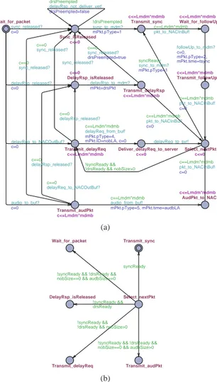
The medium is responsible for data transmission, so whenever there is available data waiting to be transmitted, the transmission must take place unless
the medium is currently busy. In a heterogeneous
system, the transmission decision is more complex as different packets have different priorities. Only the packet with the highest priority would be selected to be transmitted, others will have to backoff and wait for their turn. Figure 8(a) shows a simplified timed automa-ton modeling the transmission decision when many packets are available at the same time. In this figure,
sync released, delayRsp released, audio to buf, delayReq to N ACOutBuf, pkt to N ACInBuf
are modeled as broadcast channels, or more precisely, receiving edges which will synchronize with the send-ing edges whose name is exactly the same. Initially, the automaton can choose nondeterministically one receiving edge to take.
• Ifsync released was selected, the medium would
not have to care about other packets as Sync has the highest priority.
• IfdelayRsp released was selected, the medium
would look for any sign of sync-release. If there is not, it would allow the Delay Res to be delivered to the medium. However, if the sync-release hap-pens before it could actually start the transmission (c = 0), the Delay Res will backoff and give way
to the Sync transmission.
• If delayReq to N ACOutBuf was selected,
again the medium would look for signs of pack-ets with higher priorities. The Delay Req would backoff and give way to any such packet if ready.
• The similar situation happens whenaudio to buf
was selected.
When the transmission decision has already been de-cided, the medium transmits the packet for Lmdm ∗ mdmb time units where mdmb = prec is the clock
bound of the medium, and depending on the packet type the medium can take different actions upon completing its transmission:
• pT ype = 1 (Sync): the medium puts the packet
into the NAC input buffer and starts transmitting the Follow Up because it has the second highest priority. Transmit_delayReq c<=Lmdm*mdmb DelayRsp_isReleased c<=0 Sync_isReleased c<=0 AudPkt_to_NAC c<=Lmdm*mdmb Transmit_followUp c<=Lmdm*mdmb Transmit_audPkt c<=Lmdm*mdmb Deliver_delayReq_to_server c<=0 Transmit_delayRsp c<=Lmdm*mdmb Select_nextPkt c<=0 Wait_for_followUp c<=Lmdm*mdmb Transmit_sync c<=Lmdm*mdmb Wait_for_packet c==0 sync_released? c==0 delayRsp_released? c==0 delayReq_to_NACOutBuf? c==0 sync_released? c==0 delayRsp_released? c==0 sync_released? drsPreempted=true drsPreempted delayRsp_not_deliver_yet! drsPreempted=false !syncReady && !drsReady && nobSize>0
delayReq_to_svr! c==Lmdm*mdmb delayReq_from_buf! mPkt.pType=4, mPkt.ID=nobLA, c=0 delayReq_to_NACOutBuf? c=0 sync_released? delayRsp_to_mdm? mPkt=drsPkt delayRsp_released? c=0 syncReady sync_to_mdm? mPkt.pType=1 !drsPreempted sync_to_mdm? mPkt.pType=1 sync_released? c=0 c==Lmdm*mdmb pkt_to_NACInBuf! c=0 c==Lmdm*mdmb audio_from_buf! mPkt.pType=5, mPkt.time=audbLA c==Lmdm*mdmb pkt_to_NACInBuf! c=0 c==Lmdm*mdmb pkt_to_NACInBuf! c=0 followUp_to_mdm? c=0, mPkt.pType=2, mPkt.time=tsync audio_to_buf? c=0 c==Lmdm*mdmb pkt_to_NACInBuf! (a) Wait_for_packet Transmit_audPkt Transmit_delayReq Select_nextPkt DelayRsp_isReleased Transmit_sync
!syncReady && !drsReady && nobSize==0 && audbSize==0
!syncReady && !drsReady && nobSize==0 && audbSize>0 !syncReady &&
!drsReady && nobSize>0 !syncReady && drsReady
syncReady
(b)
Figure 8: A simplified automaton of the medium
• pT ype = 3 (Delay Res): the medium puts the
packet to the NAC input buffer.
• pT ype = 4 (Delay Req): the medium confirms its
transmission so that the packet is safely removed from the NAC output buffer and delivered to the server.
• pT ype = 5 (Audio): likewise, the audio packet
is removed from the audio buffer and put into the NAC input buffer.
The NAC input and output buffer will be discussed later. For every buffer, there is a look ahead variable that always points at the first element of the buffer when it is not empty, such asnobLA and audbLA - the look
Check_timeZero c1<=0 Transmit_delayReq c<=Lmdm*mdmb DelayRsp_isReleased c<=0 Sync_isReleased c<=0 AudPkt_to_NAC c<=Lmdm*mdmb Transmit_followUp c<=Lmdm*mdmb Transmit_audPkt c<=Lmdm*mdmb Deliver_delayReq_to_server c<=0 Transmit_delayRsp c<=Lmdm*mdmb Select_nextPkt c<=0 Wait_for_followUp c<=Lmdm*mdmb Transmit_sync c<=Lmdm*mdmb Wait_for_packet c==0 && to==11 c>0 && from==13 drsPreempted=false c==0 && to==13 c>0 && from==15 c==0 && to==14 c>0 && from==14 delayRsp_released? fr=to/13, to=fr*13+(1-fr)*to sync_released? fr=to/11, to=fr*11+(1-fr)*to sync_released? c1=0, from=13, to=11, drsPreempted=true delayRsp_released? c1=0, from=14, to=13 sync_released? c1=0, from=14, to=11 delayRsp_released? c1=0, from=15, to=13 sync_released? c1=0, from=15, to=11 delayReq_to_NACOutBuf? c1=0, from=15, to=14 drsPreempted delayRsp_not_deliver_yet! drsPreempted=false !syncReady && !drsReady && nobSize>0
delayReq_to_svr! c==Lmdm*mdmb delayReq_from_buf! mPkt.pType=4, mPkt.ID=nobLA, c=0 delayReq_to_NACOutBuf? c=0 !syncReady && drsReady sync_released? delayRsp_to_mdm? mPkt=drsPkt delayRsp_released? c=0 syncReady sync_to_mdm? mPkt.pType=1 !drsPreempted sync_to_mdm? mPkt.pType=1 sync_released? c=0
!syncReady && !drsReady && nobSize==0 && audbSize==0 c1=0
!syncReady && !drsReady && nobSize==0 && audbSize>0
c==Lmdm*mdmb pkt_to_NACInBuf! c=0 c==Lmdm*mdmb audio_from_buf! mPkt.pType=5, mPkt.time=audbLA c==Lmdm*mdmb pkt_to_NACInBuf! c=0 c==Lmdm*mdmb pkt_to_NACInBuf! c=0 followUp_to_mdm? c=0, mPkt.pType=2, mPkt.time=tsync audio_to_buf? c=0 c==Lmdm*mdmb pkt_to_NACInBuf!
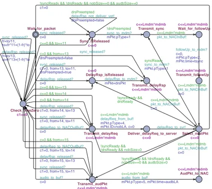
Figure 9: A complete automaton of the medium
ahead variables of the NAC output buffer and the audio buffer respectively.
Now that the automaton is selecting the next packet to transmit, if:
• syncReady (Sync is ready): the medium starts the
Sync transmission.
• !syncReady && drsReady (Delay Res is ready):
the medium starts the Delay Res transmission.
• !syncReady && !drsReady && (nobSize>0)
(Sync and Delay Res not ready and the NAC out-put buffer not empty): the medium starts the De-lay Req transmission.
• !syncReady && !drsReady && (nobSize==0) &&
(audbSize>0) (only audio packets are ready): the
medium starts the Audio transmission.
• !syncReady && !drsReady && (nobSize==0)
&& (audbSize==0) (no packet is available): the medium goes back to the initial state.
Figure 8(b) depicts these next packet selections. The complete medium automaton would be obtained by joining the states and edges in figure 8(a) and fig-ure 8(b). However, since UPPAAL does not allow clock
guards on receiving edges of broadcast channels, we have to add one more state to check the time at which the preemption happens. Figure 9 shows the complete medium automaton.
3.4
Network Access Controllers (NACs)
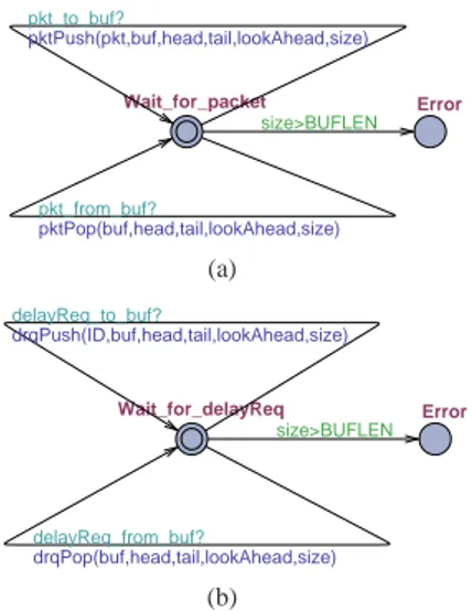
The NACs is responsible for data routing from the server into subnet(s) and vice versa. Also, the NACs can perform data encryption/decryption on every packet passing through it. Because only one packet can be pro-cessed at a time, NACs are assumed to have two buffers to contain incoming or outgoing packets. The NAC input buffer contains packets coming only from the medium and the NAC output buffer contains only De-lay Req packets going from the devices to the medium. These buffers are depicted in figure 10.
The input automaton will add or remove a packet by taking the packet to buf or packet f rom buf
tran-sition respectively. Similarly, the output automaton will add or remove a Delay Req message by taking thedelayReq to buf or delayReq f rom buf
respec-tively. In this figure,pkt denotes the incoming packet
and ID the identity of the device sending the
corre-Error Wait_for_packet size>BUFLEN pkt_from_buf? pktPop(buf,head,tail,lookAhead,size) pkt_to_buf? pktPush(pkt,buf,head,tail,lookAhead,size) (a) Error Wait_for_delayReq size>BUFLEN delayReq_from_buf? drqPop(buf,head,tail,lookAhead,size) delayReq_to_buf? drqPush(ID,buf,head,tail,lookAhead,size) (b)
Figure 10: The NAC input and output buffer
sponding automaton goes to the Error state.
Similar to the medium case, the NACs always transmit packets of the highest priority among the ready packets. Figure 11 shows a simplified timed au-tomaton modeling the activities of a NAC. In this figure,
pkt to buf, delayReq released, delayReq to extBuf
are receiving edges of broadcast channels while
delayReq to buf, pkt to subnet are emitting edges of
broadcast channels. Initially, the automaton can choose nondeterministically one receiving edge to take.
• Ifpkt to buf was selected, the NAC looks further
at the packet type. If it was either a Sync, Fol-low Up or Delay Res message (pT ype <= 3),
the NAC ignores other packets and goes on pro-cessing the current packet. In case the Delay Req from the device is preempted by the current packet, the NAC tells its attached device to back-off the Delay Req by synchronizing on the chan-neldelayReq stayin device. On the contrary, if
it was an Audio packet then the NAC would still ignore other packets as long as no Delay Req from the attached device is ready (drqReady==true) or preempted (drqSrc==1) and no Delay Req from external NACs is ready (nextbSize==0). Assum-ing that the Delay Req from the attached device has a higher priority than that from external NACs, so when they are ready at the same time the former preempts the latter.
• If delayReq released was selected, the NAC
Process_extDrq c<=Lnac*nb Process_intDrq c<=Lnac*nb Process_audPkt c<=Lnac*nb IntDrq_isReceived c<=0 Process_svrPTPpkt c<=Lnac*nb Select_nextPkt c<=0 Deliver_svrPkt c<=0 SvrPkt_isReceived c<=0 Wait_for_packet c==0 pkt_to_buf? c==0 pkt_to_buf? c==0 delayReq_released? c==0 delayReq_released? c==0 delayReq_to_extBuf? drqSrc=2 c==Lnac*nb delayReq_from_extBuf! ID=nextbLA c==Lnac*nb delayReq_to_buf! c=0, drqSrc=0
nibLA.pType==5 && !drqReady && drqSrc!=1 && nextbSize>0 drqSrc=2 nibLA.pType==5 && drqSrc==1 nibLA.pType==5 && drqReady delayReq_to_extBuf? c=0, drqSrc=2 pkt_to_buf? c==0 delayReq_from_device? ID=dvID, drqSrc=1 delayReq_released? c=0 c==Lnac*nb pkt_from_buf! c=0 nibSize>0 nibLA.pType<=3 && drqSrc==1 delayReq_stayin_device! nPkt=nibLA,drqSrc=0 nibLA.pType==5 && !drqReady && nextbSize==0 && drqSrc==0 nPkt=nibLA c==Lnac*nb pkt_from_buf! c=0 nibLA.pType<=3 && drqSrc !=1 nPkt=nibLA pkt_to_subnet! pkt_to_buf? c=0 (a) Process_extDrq IntDrq_isReceived Select_nextPkt SvrPkt_isReceived Wait_for_packet nibSize==0 && !drqReady && nextbSize>0 nibSize==0 && drqReady nibSize>0 nibSize==0 && !drqReady && nextbSize==0 (b)
Figure 11: A simplified automaton of the NACs
would look for any sign of incoming packets. If there is not, it would process the Delay Req from its attached device. Otherwise, only when the in-coming packet has a higher priority will the De-lay Req backoff.
• If delayReq to extBuf was selected (another
Delay Req is coming from an external NAC out-put buffer), again the NAC would look for signs of packets with higher priorities. The Delay Req would backoff and give way to any such packet if it is available.
When the NAC has made its decision, it will process the packet forLnac ∗ nb time units where nb = prec
is the clock bound of the NAC. After that, the NAC can take different actions upon completing processing, de-pending on whether the packet is incoming or outgoing:
• For incoming packets: the NAC confirms its
in-put buffer that the packet has been processed suc-cessfully so that the packet can be safely removed from the input buffer by synchronizing on the
pkt f rom buf channel. The packet is then
for-warded to the subnets (including external NACs and devices).
• For outgoing packets: if it was an external De-lay Req from an external source, the NAC needs to confirm the external buffer from which the lay Req is safely removed. After that, the De-lay Req is put into the NAC output buffer and waiting for the medium to take it. In addition, the identity of the device (dvID) should be included
inside the Delay Req message so that when it is received, the server could send back a Delay Res. The look ahead variables for the NAC internal in-put, internal output and external output buffer are
nibLA, nobLA and nextbLA respectively.
Now that the automaton is selecting the next packet to process, if:
• nibSize>0 (the NAC input buffer is not empty): the
NAC tries processing incoming packets.
• (nibSize==0) && drqReady (the NAC input buffer
is empty but a Delay Req from its attached device is ready): the NAC takes the Delay Req in.
• (nibSize==0) && !drqReady && nextbSize>0
(only Delay Req from external NAC output buffer is ready): the medium tries processing the external Delay Req.
• (nibSize==0) && !drqReady && (nextbSize==0)
(nothing to process): the NAC goes back to its idle state and waits for new packets.
Figure 11(b) depicts these selections. The complete NAC automaton would be obtained by joining the states and edges in figure 11(a) and figure 11(b). However, as in the medium case, since UPPAAL does not al-low clock guards on receiving edges of broadcast chan-nels, we have to add one more state to check the time at which the preemption happens. Figure 12 shows the complete NAC automaton.
Check_timeZero c1<=0 Process_extDrq c<=Lnac*nb Process_intDrq c<=Lnac*nb Process_audPkt c<=Lnac*nb IntDrq_isReceived c<=0 Process_svrPTPpkt c<=Lnac*nb Select_nextPkt c<=0 Deliver_svrPkt c<=0 SvrPkt_isReceived c<=0 Wait_for_packet c==Lnac*nb delayReq_from_extBuf! ID=nextbLA c==Lnac*nb delayReq_to_buf! c=0, drqSrc=0 c==0 && to==12 c>0 && from==14 c==0 && to==13 c>0 && from==13 c>0 && from==12 c==0 && to==11 pkt_to_buf? fr=to/11, to=fr*11+(1-fr)*to delayReq_released? fr=to/12, to=fr*12+(1-fr)*to delayReq_to_extBuf? c1=0, from=14, to=13 delayReq_released? c1=0, from=14, to=12 pkt_to_buf? c1=0, from=12, to=11 delayReq_released? c1=0, from=13, to=12 pkt_to_buf? c1=0, from=13, to=11 nibSize==0 && !drqReady && nextbSize>0 drqSrc=2
nibSize==0 && drqReady
nibLA.pType==5 && !drqReady && drqSrc!=1 && nextbSize>0 drqSrc=2 nibLA.pType==5 && drqSrc==1 nibLA.pType==5 && drqReady delayReq_to_extBuf? c=0, drqSrc=2 pkt_to_buf? c==0 delayReq_from_device? ID=dvID, drqSrc=1 delayReq_released? c=0 c==Lnac*nb pkt_from_buf! c=0 nibSize>0 nibLA.pType<=3 && drqSrc==1 delayReq_stayin_device! nPkt=nibLA,drqSrc=0 nibLA.pType==5 && !drqReady && nextbSize==0 && drqSrc==0 nPkt=nibLA nibSize==0 && !drqReady && nextbSize==0 c1=0 c==Lnac*nb pkt_from_buf! c=0 nibLA.pType<=3 && drqSrc !=1 nPkt=nibLA pkt_to_subnet! pkt_to_buf? c=0
Figure 12: A complete automaton of the NACs
3.5
Device
The device is modeled as a network of four timed automata, one of which models the device integer clock, two of which model the PTP protocol running in the device and the other models the audio receiver.
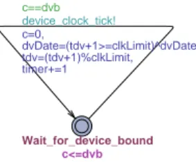
Wait_for_device_bound c<=dvb c==dvb device_clock_tick! c=0, dvDate=(tdv+1>=clkLimit)^dvDate, tdv=(tdv+1)%clkLimit, timer+=1
Figure 13: The integer clock of devices The timed automaton modeling the device integer clock is shown in figure 13. At the beginning the clock bound of the device is dvb = prec ∗ 100/edv where prec is the digit precision and edv is the device clock
drift. When clockc reaches the bound, the device
in-teger clock tdv will increase by 1 and c is reset to
Check_pType c1<=0 Find_negativeX c1<=0 Find_positiveX c1<=0 Adjust_clock c1<=0 Wait_for_followUp Wait_for_sync c>=(off-2*x)*prec*50/edv clock_adjusted! fastClock(edv,off,tdv,timer,dvb,dvDate,st,sd,x) c<(2+2*x+off)*prec*50/edv clock_adjusted! slowClock(edv,off,tdv,timer,dvb,dvDate,st,sd,x) pType>1 pType==1 t=tdv, d=dvDate pkt_to_subnet? c1=0, pType=nPkt.pType c>=(2+2*x+off)*prec*50/edv x+=1 adjust && (c>=(2+off)*prec*50/edv) clock_adjusted! x=0 c<(off-2*x)*prec*50/edv x+=1 adjust && (c<off*prec*50/edv) clock_adjusted! x=0 adjust && (c>=off*prec*50/edv) && (c<(2+off)*prec*50/edv) clock_adjusted! dvb=(2+off)*prec*50/edv !adjust pkt_to_subnet? updateT12(t1,t2,t3,t4,nPkt.time,t,d,off,adjust), c1=0
Figure 14: The first two steps of the PTP protocol run-ning in devices
reaches the clock limit clkLimit, it will be reset to
0. Also the device date is encoded in the variable
dvDate which results from the binary operation XOR: dvDate = (tdv + 1 >= clkLimit) XOR dvDate. In
addition, there is atimer keeps increasing in the figure.
We will see later how this variable is used.
The first two steps of the PTP protocol running in the device are depicted in figure 14. The device waits un-til a Sync message arrives and records the arrival date and time of the Sync. Then when a Follow Up comes, it checks whether the Sync sending and receiving ac-tions happen in a same day (this is a constraint added to simplify the modeling of PTP). If it is the case, the device further checks whether the slave-to-server delay is available (t4 > 0). Then if such delay is not
avail-able, the device goes back to its initial state. Otherwise, it proceeds with the clock adjustment. The auxiliary procedures updateT12 helps the device in making its adjustment decision.
The current scaled time point istdv ∗ prec + edv ∗ c/100 (tdv and c are two shared variables of the
in-teger clock timed automaton), after clock adjusting it becomestdv ∗ prec + edv ∗ c/100 − of f ∗ prec/2 =
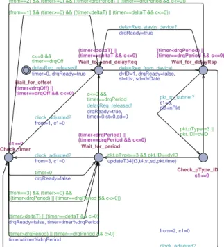
Check_timer c1<=0 Wait_for_period (timer<drqPeriod) || (timer==drqPeriod && c<=0) Check_pType_ID c1<=0 Wait_for_delayRsp (timer<drqPeriod) || (timer==drqPeriod && c<=0) Wait_to_send_delayReq (timer<deltaT) || (timer==deltaT && c<=0) Wait_for_offset (timer<drqOff) || (timer==drqOff && c<=0)
(timer>deltaT) || (timer==deltaT && c>0) drqReady=false, timer=timer%drqPeriod (from==3) && (timer>=0) &&
((timer<drqPeriod) || (timer==drqPeriod && c<=0)) timer<0
drqReady=false
(from==1) && (timer>=0) && ((timer<deltaT) || (timer==deltaT && c<=0))
clock_adjusted? from=1, c1=0
clock_adjusted? from=2, c1=0 (from==2) && (timer>=0) && ((timer<drqPeriod) || (timer==drqPeriod && c<=0))
(timer>drqPeriod) || (timer==drqPeriod && c>0) timer=timer%drqPeriod clock_adjusted? from=3, c1=0 delayReq_stayin_device? drqReady=true c<=0 && timer==drqPeriod delayReq_released! drqReady=true, timer=0,st=0,sd=0
pkt.pType==3 && pkt.ID==dvID updateT34(t3,t4,st,sd,pkt.time) pkt.pType!=3 || pkt.ID!=dvID pkt_to_subnet? c1=0, pkt=nPkt delayReq_from_device! dvID=1, drqReady=false, st=tdv, sd=dvDate c<=0 && timer==drqOff delayReq_released! timer=0, drqReady=true
Figure 15: The last two steps of the PTP protocol run-ning in devices
Procedure 2 updateT12(int &t1, int &t2, int &t3, int
&t4, int &tsend, int &trecv, int &recvDate, int &off, bool &adjust)
1: int sendDate=(tsend>=clkLimit); 2: adjust=false; 3: if sendDate==recvDate then 4: t1=tsend-sendDate*clkLimit; 5: t2=trecv; 6: if t4>0 then 7: adjust = true; 8: end if 9: if adjust then 10: off+=t2+t3-t1-t4; 11: end if 12: end if 13: trecv=0; 14: recvDate=0;
tdvnew∗prec+delta where 0 <= delta < prec. There
are three possibilities:
• 0 <= (edv ∗ c/100 − of f ∗ prec/2) < prec or (of f ∗ prec ∗ 50/edv) <= c < [(2 + of f ) ∗ prec ∗ 50/edv] ⇒ tdvnew = tdv and dvbnew =
• (edv ∗ c/100 − of f ∗ prec/2) < 0 or c < (of f ∗ prec∗50/edv) ⇒ the device clock is running faster
than the server clock and so there exists x > 0
such that0 <= tdv ∗ prec + edv ∗ c/100 − of f ∗ prec/2 + x ∗ prec < prec and tdvnew= tdv − x
anddvbnew= [(2 − 2 ∗ x + of f ) ∗ prec ∗ 50/edv]
• (edv ∗ c/100 − of f ∗ prec/2) >= prec or c >= [(2 + of f ) ∗ prec ∗ 50/edv] ⇒ the device clock is
running slower than the server clock and so there existsx > 0 such that 0 <= tdv ∗ prec + edv ∗ c/100 − of f ∗ prec/2 − x ∗ prec < prec and tdvnew = tdv + x and dvbnew = [(2 + 2 ∗ x +
of f ) ∗ prec ∗ 50/edv]
Moreover, the delayReq-release task has the pe-riod of drqP eriod and may have some initial offset drqOf f . After the delayReq-release event is acti-vated, the Delay Req message must be delivered to the medium withindeltaT ∗ dvb time units. The time when
the Delay Req has been taken in by the NAC should be recorded so that it will be used later in the PTP protocol. Figure 15 shows the last two steps of the synchro-nization procedure in the devices. In this figure, all edges are normal channels exceptdelayReq released
andclock adjusted - two broadcast channels.
After at mostdrqP eriod ∗ dvb time units since the
Delay Req delivery, the Delay Res message has to be received by the device according to the PTP protocol. These timing constraints are enabled by using a timer. This is because the device clock bound is changed pe-riodically and not static as the server clock bound. Ad-ditionally, the timer is put forward or backward the same amount of time as the local clock is. So after the clock adjustment, if the timer does not respect the invariants any longer, the automaton will abort the ac-tivity it was taking before the clock adjustment took place. For example, if (timer<0) or (timer>deltaT) or
((timer==deltaT)&& (c>0)) (c is a shared variable of
the integer clock timed automaton), it cancels the cur-rent delivery and waits to start a new Delay Req de-livery. If no invariant violations is committed, the au-tomaton executes its normal cycle, that is sending a lay Req to the server, receiving the corresponding De-lay Res and updating the slave-to-master deDe-lay infor-mation. The auxiliary procedure updateT34 helps with the last step in the cycle, assuming that the Delay Req sending and Delay Res receiving actions should hap-pen in a same day (this is another constraint added to simplify the modeling of PTP).
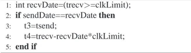
Procedure 3 updateT34(int &t3, int &t4, int &tsend,
int &sendDate, int &trecv)
1: int recvDate=(trecv>=clkLimit); 2: if sendDate==recvDate then
3: t3=tsend;
4: t4=trecv-recvDate*clkLimit; 5: end if
Lastly, figure 16 describes the audio receiving opera-tion of the device. The date and time informaopera-tion of the audio packet is retrieved and checked with the current date and time of the device local clock. If the clock has passed the time at which the packet must be played, the automaton will go to the Error state.
Check_pType c<=0 Error Check_deadline c<=0 Wait_for_audPkt pkt.pType<5 pkt.pType==5 audDate=(pkt.time>=clkLimit), pkt.time-=clkLimit*audDate pkt_to_subnet? c=0, pkt=nPkt dvDate!=audDate || pkt.time>=tdv audDate=0,pkt.pType=0, pkt.ID=0,pkt.time=0 dvDate==audDate && pkt.time<tdv
Figure 16: The audio receiver of devices
4
Ground Verification
The above models have been validated by UPPAAL, a model-checker for timed-automata [4]. In the pre-vious section, all of the models were constructed in the syntax of UPPAAL. Thus, it is trivial to feed them directly to UPPAAL so that their properties can be
checked by the verifier of the tool. UPPAAL uses
a timed Computation Tree Logic (CTL) language for specifying properties which we want to verify. To ver-ify that the system is schedulable, we must show that the four error states are never reachable. Using the timed CTL language, the schedulability properties are speci-fied as follows:
• A[]!SVR AudBuf.Error
• A[]!NACInBuf.Error
• A[]!NACOutBuf.Error
Only if these schedulability properties are satisfied, can we be sure that the system is schedulable. If just one property is violated, the system is not guaranteed to work properly because it may encounter the dead-lock state where none of the timed automata can move. Several test cases are performed to illustrate this point. In the first test case, the schedulability of the system is guaranteed because all properties are satisfied while it is not in the second case due to the violation of the last property. The last test case points out the possibility of deadlock when the second property is not satisfied. In all test cases, the system consists of one server, one medium, one NAC and one device.
4.1
Test case 1
In this test case, the Sync interval and the period of the Delay Req message are equal to 20ms while that of the Audio packets is 40ms. The offset parameters are 0 for the sync and audio packets and 10ms for the Delay Req message. Moreover, the latency parameters of the medium and the NACs are assumed to be 1ms, the clock drifts for the server and its device to be 0.99 and 0.95 correspondingly. Other parameters are also given fixed values such as deltaT=10ms, relD=10ms, BUFLEN=5 (elements), prec=10 (hence the digit pre-cision is 1), clkLimit=100. Because of the small preci-sion, at the beginning, the clock bound is the same in all environments. That is, svrb=dvb=mdmb=nb=10.
In figure 17 and figure 18, we show the task execu-tion scheme of the system. The Sync, Follow Up and Audio packets are delivered to the medium at time 0, 1 and 2 respectively. They are then forwarded to the NAC at time 1, 2 and 3 respectively by the medium. At time 10 a Delay Req message is released by the de-vice and since the NAC is currently free, the message is processed immediately and transmitted to the medium at time 11. After receiving the Delay Req, the server sends out the Delay Res message at time 12 and the de-vice receives the message at time 14. This execution scheme is repeated at time 20, 40, 60, etc.
In the first cycle, since the Sync and Follow Up mes-sages arrived when no Delay Req had been sent by the device, its local time is not adjusted. In the next cycle, when the Sync and Follow Up messages arrive once again, the offset can now be computed as all parameters needed for clock synchronization are available. In this special case, the master-to-slave and slave-to-master de-lays are equal to 2, thereby zeroing the offset and letting the device clock remain unchanged.
Figure 17: Task execution scheme of the medium(test1)
Figure 18: Task execution scheme of the NAC(test 1)
The first audio packet arrived at the device at time 4 which perfectly respects its deadline at time 10. The next audio packets would arrive at time 44, 84, etc. which will also respect their deadline of 50, 90, etc. In addition, the sizes of the audio buffer, the NAC input buffer and output buffer never exceed 1. Thus, all the schedulability properties are verified and the schedula-bility of the system can be guaranteed.
4.2
Test case 2
In this test case, the Audio packets are generated more frequently and its period is 5ms while the Sync interval and the Delay Req period are 20ms and 40ms respectively. All these packets have offset 0 and the audio relative deadline is 15. Moreover, the medium latency (which is 2ms) is a little longer than the NAC latency (which is 1ms). Other parameters take the same values as in the previous test case.
Before bumping into the Error state of the
DV AudRecvr timed automaton, two clock
adjust-ments had happened as shown in table 1.
At time 0, the clock bound is the same in all envi-ronments, namely svrb=dvb=mdmb=nb=10 due to the 1-digit-precision as in the previous case. The Sync is sent at time 0 by the server and received at time 3 by the device. Since the slave-to-master delay is not available yet, the first clock adjustment does not actually happen.
1st 2nd 3rd svrb 10 10 10 dvb 10 10 5 mdmb 10 10 10 nb 10 10 10 t1 0 20 na t2 3 23 na t3 0 0 40 t4 0 6 35 of f = t2+ t3−t1−t4 0 -3 -1
Table 1: The clock adjustments happen before the au-tomaton goes to the Error state
Audio sending 0 5 10 15 20 25 30 35
Audio receiving 11 13 15 18 27 34 44 56
Time to play 15 20 25 30 35 40 45 50
Deadline violation No No No No No No No Yes
Table 2: Deadline violation of audio packets
It is noticeable that the Delay Req was released at time 0 and got out of the NAC at time 1, but because of its low priority compared to the Sync and Follow Up mes-sages, it has to wait until the higher priority messages pass through the medium. Thereby adding a delay to its arrival at the server which is finally 6.
At time 20, the Sync is released once again and since it has the highest priority, it arrives at the device at time 23. Now that the master-to-slave and slave-to-master delays are available, we can perform the offset calcula-tion. In fact, the device clock is 1.5 ms behind. How-ever, since UPPAAL does not support the real type, the offset is integerize advancing the device clock from 25 to 26 and changing the device bound from 10 to 5 as a result. After that, an audio-deadline violation takes place at time 56 before the third adjustment has hap-pened.
Table 2 summarizes the times at which the audio packets are released, received and played. It is impor-tant to notice that the device clock has been adjusted at time 25 and elapsing two times faster than the server clock since then. And before it could be adjusted to elapse at the slower speed, it has caused one audio packet to violate its deadline.
4.3
Test case 3
In this test case, the medium latency (which is 2ms) is a much shorter than the NAC latency (which is 6ms). Other parameters take the same values as in the previous test case.
Figure 19: Task execution scheme of the medium(test3)
Figure 20: Task execution scheme of the NAC (test 3)
In figure 19 and figure 20 we show the task execution scheme of the system. The Sync, Follow Up and the first Audio are delivered to the medium at time 0, 2 and 4 respectively. Also at time 0, a Delay Req message is released by the device and since the NAC is currently free, the message is processed immediately. At time 6, the Delay Req enters the medium while the Sync enters the NAC. After receiving the Delay Req at time 8, the server sends out the Delay Res message immediately. At time 10 and 12, two other Audio packets which were released at time 5 and 10 are transmitted by the medium to the NAC. Also at time 12, the NAC finishes process-ing the Sync and starts processprocess-ing the Follow Up. At time 15, another Audio packet is released and it arrives at the NAC at time 17 by which the NAC input buffer has overflowed because it is currently contains one Fol-low Up, one Delay Res and three other Audios. As a result, the system will soon encounter the deadlock state because when the medium has other Audio packets to forward to the NAC, it could not synchronize with the NAC input buffer automaton as the automaton is cur-rently staying in the Error state.
Wait_for_period c<=ptpPeriod Wait_for_offset c<=ptpOff c==ptpPeriod Release_PTP! c=0 c==ptpOff Release_PTP! c=0 (a) Wait_for_period c<=audPeriod Wait_for_offset c<=audOff c==audPeriod Release_Audio! c=0 c==audOff Release_Audio! c=0 (b)
Figure 21: PTP and audio task activation automata
5
Parametric Analysis
The UPPAAL timed automata in section 3 are very specific models which follow closely the operations of the HCS system (including the server, the medium, the NACs, the devices and the PTP protocol) given in sec-tion 2. If the details of those operasec-tions are abstracted from the system models, we will obtain abstract models describing the system at a higher level. For instance, the abstract model for the devices would be a periodic task set consisting of the PTP task and the audio receiver task. The PTP task has a higher priority than the au-dio receiver task as specified in section 2. In addition, the execution time of the former accounts for the total PTP load that the devices could bear and that of the lat-ter accounts for the total delay of traversing through the medium and the NACs of the audio packets.
With all the UPPAAL models developed previously, it is now easier for the system designer to verify if there is any deadline miss with respect to the audio packets, given a fixed set of parameters. It could even be more helpful to the system designer if he could be provided with the parametric analysis on the abstract models of the system. These models gain the advantage of small complexity in applying the PTA tool over the specific models. In this section, the parametric analysis is car-ried out only on the abstract models of the devices to identify the parameter space that can guarantee to re-spect the deadline of audio packets and PTP packets. The analysis on the abstract models of the server could be done similarly. Error Busy Check Idle Release_Audio? c==0 && task==2 Release_PTP? r=r+C1+C1*n1-C2 c==r && n1==0 && n2>0 r=C2, task=2, c=0, n2=n2-1 c==r && n1>0 r=C1, task=1, c=0, n1=n1-1 c==0 & task==2 Release_PTP? task=1, r=C1, n2=n2+1 c<r && c==D1 Release_PTP? (c<r) && (c>0 || task==1) Release_PTP? r=r+C1+C1*n1-c, c=0 c<r Release_Audio? n2=n2+1 (c<r) && (c>0 || task==1) Release_PTP? n1=n1+1 c==r && n1==0 && n2==0 Release_PTP? task=1, c=0, r=C1, n1=0, n2=0 Release_Audio? task=2, c=0, r=C2, n1=0, n2=0 c==r && c<=D1 Release_PTP? c=0, r=C1
Figure 22: Schedulability checker for task PTP
5.1
Abstract Models
The activation automata for the PTP and audio receiver tasks are shown in figure 21. The offset, period and deadline are fixed for each task.
Based on the checkers used in [2], the schedulability checkers for the two tasks are modified to model a non-preemptive scheduling environment. That is, the audio packets can not be preempted by the PTP packets if they are currently being transmitted by the network or pro-cessed by the NACs. The preemption can only happen when the audio packets have just been released and not transmitted yet. So, when many packets are ready at the same time, the PTP would go first and the audio would back off.
The scheduler checker for the PTP task is shown in figure 22. In this figure, D1 is the deadline of the PTP task which is less than or equal to the PTP period, C1 and C2 are the execution time of the PTP and audio tasks respectively.
This checker differs from the checker in [2] in the following details.
• Firstly, three additional variables are introduced.
The variable task denotes the currently-executed task, n1 and n2 record respectively the number of PTP and audio packets released during the current execution.
• Secondly, at location Busy, when one task is be-ing executed (c>0), other task instances will be
can only take place in the situation where the audio task is about to be executed (c==0 && task==2) when the PTP task is ready for execution.
• Thirdly, the additional self-loops at location Busy are taken when the current execution is completed. If the PTP queue is not empty (n1>0), a PTP
in-stance will be removed from the queue and then executed. Otherwise, an audio instance will be scheduled as long as n2>0. If both queues are
empty, the transition from Busy to Idle is taken, indicating no tasks are ready to be executed.
• Lastly, transitions entering Check from Busy
are taken when a PTP instance is
(non-deterministically) chosen for checking. Again, the preemption can happen if the transition is taken at c==0 and the task about to be executed is the audio task. Moreover, before any deadline verification, the execution time of all other PTP instances in the queue must be taken into account as they would be scheduled before the current PTP instance, that is r should be updated to c) or (r+C1*n1-C2). Error Busy Check Idle Release_Audio? c<r && c==D2-driftDelta c>0 && c<r && c<D2-driftDelta Release_PTP? c==0 Release_PTP? r=r+C1 c<r Release_Audio? r=r+C2-c, c=0 c<r Release_Audio? r=r+C2 c<r Release_PTP? r=r+C1 c==r Release_PTP? c=0, r=C1 Release_Audio? c=0, r=C2 c==r && c<=D2-driftDelta Release_Audio? c=0, r=C2
Figure 23: Schedulability checker for task Audio Re-ceiver (hard deadline)
The scheduler checker for the audio receiver task is shown in figure 23. Similarly, the Release PTP transi-tions are added to the Check state to ensure that when an audio transmission is going on (c>0), the PTP would
back off and if that transmission is about to happen (c==0), the PTP can preempt it (r=r+C1). In the
fig-ure, D2 is the relative deadline of audio packets. Be-sides, the parameter driftDelta is introduced to account for the offset time of the local clock compared to the server clock. The worst case happens when the local clock is substantially slower than the server clock and thus when an audio packet is received, the actual dead-line to be verified would be D2-driftDelta instead of D2. In fact, the requirement of no deadline miss is dif-ficult to obtain in real-time environments. Therefore, in order to make the analysis more practical, the re-quirement can be relaxed by allowing an audio packet to sometimes miss its deadline. However, there should be no other deadline miss after one is made. In other words, the situation of two successive deadline misses should never happen. The checker adapted for this new requirement is shown in figure 24.
In the figure, three new variables are introduced. One is the boolean variable dm used to capture the fact that one deadline miss has already happened (dm=true), the others are the real variable r1 and r2 used to record re-spectively the total execution time of all PTP instances released between two consecutive audio instances and of the latter audio instance, if it is released before a deadline miss. This checker is also different from the
Check2
Error
Busy
Check1 Idle
c==r && c<=D2-driftDelta c<r && c==D2-driftDelta
r2>0 && !dm && c<r && c==D2-driftDelta r=r+r1+r2-c, c=0 r2>0 Release_Audio? r2>0 && c>t && c<r && c<D2-driftDelta Release_PTP? r2>0 && c==t Release_PTP? r1=r1+C1 r2==0 && !dm && c<r && c==D2-driftDelta dm=true, r=r+r1 r2==0 && c<r && c<D2-driftDelta Release_Audio? r2=C2, t=c dm && c<r && c==D2-driftDelta r2==0 && c>0 && c<r && c<D2-driftDelta Release_PTP? r1=r1+C1 c==0 Release_PTP? r=r+C1 c<r Release_Audio? r=r+C2-c, c=0, r1=0, r2=0 c<r Release_Audio? r=r+C2, dm=false c<r Release_PTP? r=r+C1 c==r Release_PTP? c=0, r=C1 Release_Audio? c=0, r=C2 c==r && c<=D2-driftDelta dm=false Release_Audio? c=0, r=C2, r1=0, r2=0
Figure 24: Schedulability checker for task Audio Re-ceiver (soft deadline)
Experiment 1 Experiment 2 ptpOf f 0 5 ptpP eriod 40 40 D1 10 10 audOf f 0 0 audP eriod 10 10 D2 10 10
Table 3: Fixed parameter values in two experiments
transitions from Check1 to other locations and the in-troduction of the new location Check2.
Transitions entering Check1 from Idle or Busy are taken when an audio instance is (non-deterministically)
chosen for checking. And if another PTP instance
is also ready before this audio instance is executed (c==0), it would be preempted (r=r+C1). Then the execution time of all other PTP instances would be ac-cumulated until another audio instance is released or it misses its deadline.
When the current audio instance finally violates its deadline:
• If one deadline miss had happened before
(dm=true), the location Error is reached because of two successive deadline misses.
• Otherwise, if another audio instance has already been released (r2>0), the transition from Check1
to Check2 is taken in order to verify if it would miss its deadline the second time.
• If there was no deadline miss (dm=false) and no
other audio instance is released before the current deadline miss, the variable dm is updated to true and the transition from Check1 to Busy is taken to tolerate the first deadline miss.
5.2
Experiments
In this section, we report on the results of experi-menting the above periodic task set on the PTA imple-mented in [2]. The following information is used as the initial constraints: C1> 0 C2> 0 C1<= D1 C2<= D2 driftDelta>= 0
In both experiments, we use bounded model
check-ing with the bound of 60 to find the feasibility region for
C1 C2 drif tDelta
Table 4: Free parameters of the system Experiment 1 Experiment 2
CheckerP T P 62 90
CheckerAudio 2 15
Table 5: Running time in minutes in two experiments
the system. Table 3 shows the values of all fixed param-eters in two experiments while the free paramparam-eters are specified in table 4. Moreover, the running time results of the two experiments are summarized in table 5. The computer used in the experiments has 1GB RAM and Intel Core 2 Duo CPU T7500 2.20 GHz. It is notice-able that the PTP checker generally runs much slower than the Audio checker which may be because the path leading to the error state of the former is much longer than that of the latter. The running time also depends on the bound used to model check the system. Using a large bound can help to find more traces to the error state, hence the feasibility region is more correct. How-ever, the larger the bound is, the longer the running time is. So in finding the schedulable region, one must trade off between a large bound and short computation time.
Experiment 1:
For this experiment, the feasibility region in which task PTP is guaranteed to never miss its deadline is ex-pressed in the constraints below:
1: ![(C1 = 10) ∧ (15/2 < C2 <= 10)]∧ 2: ![(2 ∗ C1 + 4 ∗ C2 > 50) ∧ (C1 <= 10) ∧ (C2 <= 10)]∧ 3: ![(2∗C1+4∗C2 = 50)∧(0 < C1 < 10)∧(15/2 < C2 <= 10)]∧ 4: ![(4∗C1+8∗C2 > 90)∧(2∗C1+4∗C2 <= 50)∧ (C1+4∗C2 > 40)∧(C1 <= 10)∧(C2 <= 10)]∧ 5: ![(6 ∗ C1 + 12 ∗ C2 > 130) ∧ (3 ∗ C1 + 8 ∗ C2 <= 90)∧(C1+4∗C2 > 40)∧(C1 <= 10)∧(C2 <= 10)]
Figure 25 graphically shows the error region for each constraint. The feasibility region of task PTP is the square with a side length of 10 excluding the total er-ror region, as shown in figure 26.
By joining this region together with the schedulabil-ity region of task Audio expressed in the following
con-0 2 4 6 8 10 0 2 4 6 8 10 C2 C1 (C1=10) and (15/2<C2<=10) (a) Constraint 1 0 2 4 6 8 10 0 2 4 6 8 10 C2 C1 (2*C1+4*C2=50) (b) Constraint 2 0 2 4 6 8 10 0 2 4 6 8 10 C2 C1 (2*C1+4*C2=50) (c) Constraint 3 0 2 4 6 8 10 0 2 4 6 8 10 C2 C1 (2*C1+4*C2=50) (C1+4*C2=40) (4*C1+8*C2=90) (d) Constraint 4 0 2 4 6 8 10 0 2 4 6 8 10 C2 C1 (C1+4*C2=40) (6*C1+12*C2=130) (3*C1+8*C2=90) (e) Constraint 5
0 2 4 6 8 10 0 2 4 6 8 10 C2 C1 (C1=10) and (15/2<C2<=10) (2*C1+4*C2=50) (C1+4*C2=40) (4*C1+8*C2=90) (6*C1+12*C2=130) (3*C1+8*C2=90)
Figure 26: The total error region for task PTP (experiment 1)
straints, we would obtain the final region in which the whole system can work properly:
1: ![(dd = 10) ∧ (C1 <= 10) ∧ (0 < C2 <= 10)]∧ 2: ![(C1 + C2 + drif tDelta > 10) ∧ (0 < C1 <=
10) ∧ (C2 <= 10) ∧ (drif tDelta >= 0)]
Figure 27 shows the error region for task Audio which has a volume of 5/6 of that of the cube with a side length of 10. The remaining volume of the cube is the feasibility region for task Audio which is a tetrahe-dron as figure 27.
For example, when driftDelta = 0, the feasibility re-gion for the whole system is half of the base area of the cube which is the right triangle area with a cathetus length of 10. This can be easily verified by looking at the behaviour of the system. The first PTP released at time 0 does not miss its deadline because C2<=10.
Although the first Audio instance is preempted at time 0 by the first PTP instance, it also did not violate its deadline since C1+C2<=10. The other three Audio
in-stances released at time 10, 20 and 30 are not preempted as PTP instances are only released after 40 time unit. At time 40, the task arrival pattern is repeated with one PTP instance and one Audio instance released simul-taneously at time 40, then three other Audio instances arrive at time 50, 60 and 70. Thus, when there is no clock drift, the system is guaranteed to be schedulable as long as C1+C2<=10.
When driftDelta = 1, the feasibility region for the whole system returned by the PTA tool is bounded by the line C1+C2<=9. However, there are points that
should be in the feasibility region but got excluded by the tool finally. For example, with C1 = 5 and C2 = 5, the first Audio instance misses its deadline but the sec-ond does not which obeys the soft deadline. And the other two Audio instances at time 20 and 30 also do not miss their deadlines. Similarly for (C1 = 4, C2 = 6) or for (C1 = 3, C2 = 7) or any other pair of values for (C1,C2) that satisfy the constraint C1+C2=10. It is no-ticeable that these points are included in the feasibility region for task PTP but not for task Audio. So the result returned by the tool for task Audio seems conservative in this case which needs to be investigated to find a bet-ter solution.
Experiment 2:
For this experiment, similar to what was done in ex-periment 1, the feasibility region in which task PTP is schedulable is expressed in the following constraints:
1: ![(C1 + C2 > 15) ∧ (C1 <= 10) ∧ (5 < C2 <= 10)]∧ 2: ![(5/3 < C1 <= 5) ∧ (C2 = 10)]∧ 3: ![(40 < C1 + 4 ∗ C2 <= 45) ∧ (3 ∗ C1 + 5 ∗ C2 > 55) ∧ (C1 <= 10) ∧ (5 < C2 <= 10)]∧ 4: ![(5 ∗ C1 + 9 ∗ C2 > 95) ∧ (2 ∗ C1 + 8 ∗ C2 <= 85) ∧ (C1 + 5 ∗ C2 = 50) ∧ (C1 + 4 ∗ C2 > 40) ∧ (0 < C1 <= 10) ∧ (5 < C2 <= 10)]∧ 5: ![(1 < C1 <= 5/2) ∧ (C2 = 10)]∧ 6: ![(5 ∗ C1 + 9 ∗ C2 > 95) ∧ (2 ∗ C1 + 8 ∗ C2 <= 85) ∧ (C1 + 5 ∗ C2 <= 50) ∧ (C1 + 4 ∗ C2 > 40) ∧ (C1 <= 10) ∧ (5 < C2 <= 10)]∧ 7: ![(5 ∗ C1 + 9 ∗ C2 > 95) ∧ (2 ∗ C1 + 9 ∗ C2 > 85)∧(2∗C1+8∗C2 <= 85)∧(2∗C1+5∗C2 <= 60) ∧ (C1 + 5 ∗ C2 > 50) ∧ (C1 <= 10) ∧ (5 < C2 <= 10)]
And that of task Audio is expressed as follows: 1: ![(C1 <= 10)∧(0 < C2 <= 10)∧(drif tDelta = 10)]∧ 2: ![(C2 + drif tDelta > 10) ∧ (C1 <= 10) ∧ (C2 <= 10) ∧ (drif tDelta >= 5)]∧ 3: ![(C2 + drif tDelta > 10) ∧ (C1 <= 10) ∧ (5 < C2 <= 10) ∧ (0 <= drif tDelta < 5)]∧ 4: ![(C1 + 2 ∗ C2 + drif tDelta > 20) ∧ (C1 + C2 > 10) ∧ (C1 <= 10) ∧ (5 < C2 <= 10) ∧ (drif tDelta >= 0)]∧ 5: ![(C1 + drif tDelta > 10) ∧ (5 < C1 <= 10) ∧ (0 <= drif tDelta <= 5)]∧ 6: ![(C1 + C2 + drif tDelta > 15) ∧ (C2 + drif tDelta <= 10)∧(5 < C1 <= 10)∧(C2 <= 5) ∧ (drif tDelta >= 0)]
In this experiment, with a nonzero offset ptpOff = 5, the result becomes much more complicated because now the first PTP instance will have to experience some delay as it arrives after the first Audio instance. Thus, the trace leading to the error state will be more compli-cated and not as simple as in experiment 1.
6
Conclusions
In this report, the application of the PTA tool in [2] is studied by applying the tool to a distributed Heteroge-neous Communication System(HCS). The reports starts with describing the system and its requirements. Next, a complete set of UPPAAL models that we have built
for the system are explained fully and clearly. These models are then validated by the ground verifications. Finally, part of the system models are converted into parametric timed automata which are run to produce the schedulability regions.
In the future, we plan to extend the models to depict fully the system, such as modeling the PTP protocol in the NAC, ensuring that the audio data is played back at end devices synchronously with a given maximal jit-ter (e.g. 0.1ms), etc. The parametric timed automata would then be designed in order to capture the new re-quirements.
7
Acknowledgments
The authors would like to thank Marius Bozga for help with modeling the system, and EADS for providing the case study.
References
[1] IST STREP 215543 COMBEST, Case Study De-scription and Requirements.
[2] A. Cimatti and L. Palopoli and Y. Ramadian, Sym-bolic Computation of Schedulability Regions Us-ing Parametric Timed Automata, Real-Time Sys-tems Symposium, Nov.30 2008-Dec.3 2008. [3] H. Bowman, G. Faconti and M. Massink.
Specifi-cation and VerifiSpecifi-cation of Media Constraints using UPPAAL. 5th Eurographics Workshop on the De-sign, Specification and Verification of Interactive Systems, DSV-IS 98, Springer Verlag, 1998. [4] K. G. Larsen, P. Patterson, and Y. Wang.
UP-PAAL in a nutshell. Springer International Jour-nal of Software Tools for Technology Transfer, 1, 1997.
[5] A Precision Clock Synchronization Protocol for Networked Measurement and Control Systems. IEEE Standard 1588-2002, November 2002. [6] R. Alur and D. L. Dill. A theory of timed
automata. Theor. Comput. Sci., 126(2):183235, 1994.
[7] D. Zhang and R. Cleaveland. Fast on-the-fly para-metric real-time model checking. In RTSS05,
Washington, DC, USA, 2005. IEEE Computer So-ciety.
[8] T. Hune, J. Romijn, M. Stoelinga, and F. W. Vaandrager. Linear parametric model checking of timed automata. In TACAS 01, Springer-Verlag, 2001.
[9] Etienne Andre, Thomas Chatain, Emmanuelle En-crenaz, and Laurent Fribourg. An inverse method for parametric timed automata. Electronic Notes in Theoretical Computer Science 223 (2008).