Achieving super-realtime performance for tennis table ball tracking

Treball final de grau

GRAU DE ENGINYERIA INFORMÀTICA

Facultat de Matemàtiques i Informàtica

Universitat de Barcelona

Achieving super-realtime

performance for tennis table ball

tracking

Autor: Jordi Olivares Provencio

Director:

Dr. Eloi Puertas

Realitzat a: Departament de Matemàtiques i Informàtica

CAR, Centre d’Alt Rendiment Esportiu

Abstract

Table Tennis is inherently a sport where the ball itself moves extremely fast. In this paper, we present a super-realtime optimization of the work done by Christian Soler’s algorithm for tennis table ball and bounce detection. We also provide a proof-of-concept in the form of a C++/CUDA program that achieves rates of up to 1,000 frames per second processed.

Contents

3.2 Libraries and technologies . . . 9

3.3 Camera position . . . 10

4 Implementation 11 4.1 GPU processing . . . 11

4.1.1 Preprocessing . . . 11

4.1.2 Obtaining area of interest . . . 14

4.1.3 Post-processing . . . 15 4.2 CPU processing . . . 16 4.2.1 Ball detection . . . 16 4.2.2 Bounce detection . . . 17 5 Results 19 5.1 Testing set . . . 19 5.2 Speed of processing . . . 21 5.3 Timing metrics . . . 21 5.4 Ball detection . . . 22 5.5 Bounce detection . . . 23 6 Future Work 26 6.1 3D tracking . . . 26

6.2 Tracking multiple balls . . . 27 6.3 Implement efficient pipelining of the operations . . . 27

7 Conclusion 28

A Proof-of-concept 29

A.1 Dependencies . . . 29 A.2 Format of output . . . 29 A.3 Options . . . 29 B Performance calculators 31 B.1 Detection . . . 31 B.2 Bounce . . . 31 B.3 Timings . . . 32 References 34

Chapter 1

Introduction

Table tennis is an incredibly fast-paced sport. In most of the cases the ball can achieve speeds of up to 112 km/hour, rendering a normal 60 fps camera impractical for tracking purposes. This forces the need of a high-speed camera and subsequently the need arises for super real-time tracking if the tracking is needed to be done at the same moment. To achieve this purpose, we got help from the CAR Institute (Centre d’Alt Rendiment) in order to obtain the required video samples with real tennis table professionals.

1.1

Motivation

The purpose behind a ball and bounce detection process is motivated by the need of having accurate data for training purposes and for helping decide where a ball might have hit the table. In particular, for CAR’s case the motivation for having ball positioning would mean that they can track the position of the ball at all times. This would prove invaluable for them, as it allows their trainers to use this data in order to improve the athlete’s performance.

The reasoning for why we need a super-realtime performance comes due to the fact that the balls move at speeds of up to 112 km/hour. This renders normal cameras impractical for tracking purposes, as their rate of capture is too small. In a practical example, there were cases were the ball traveled up to one meter across the table from frame to frame. This is why there is a need for high-speed cameras. Now, since the high-speed cameras produce a torrent of data, we need to process it in order to reduce the need for storage. This is where the need for super-realtime performance is required.

As another example of the amount of data to be processed is, let’s assume a camera producing colour frames at a resolution of 350x480 and a framerate of 230 frames per second. This comes out to 350×480×3×230 = 115920000 bytes. Which is to say around 116 megabytes per second. This is just for one camera. As can be seen, since a normal

match can last for around 10 minutes, we would have to process approximately 69.5 GB per match if we only used one camera. If accurate tracking is to be done, there might be multiple cameras involved, each producing this amount of data. This is the reasoning behind the need for a super-realtime algorithm that can handle all of this data. There’s also the motivation of response time. If the system can handle all of this in realtime, it means the trainer can take decisions right then and there without having to wait for a process to execute. This would introduce an unnecessary delay which might lower the user’s experience.

1.2

Objective

The main objective set for this final degree project was originally going to be based around the idea of 3D tracking of a ball in real-time using high-speed cameras and the algorithm exposed in Christian Soler’s work [3]. As the project went along, the objective itself was changed since we couldn’t obtain more than one high-speed camera. This caused us to drop the objective of achieving 3D tracking and focus on optimizing the proof-of-concept program done by Christian Soler in order to process the high-speed-cameras in realtime.

As it turned out, the final objective would be set as achieving super-realtime performance at ball tracking and bounce detection. This performance was originally set to be at achieving a rate of 200 frames processed per second. Allowing ourselves a bit of margin in case the rate was found to be a bit too low, we internally set this to be at 300 frames per second. Personally though, the rate to achieve was doubled to 600 frames per second in order to allow future works off of the project with 3D tracking in mind. This would allow the simultaneous processing of two cameras on the same machine, thus simplifying lives for those that would come after.

1.3

Related work

Previous attempts at tracking the ball and detecting bounces were done using micro-phones with the PingPong++ [5] project.

In this project, the ball wasn’t tracked from above the table but from below it using a combination of microphones placed strategically under it. In this manner, the ball’s bounce could be detected using sound triangulation to achieve a precise location of the bounce. However, the system is very susceptible to literal noise, becoming less and less precise as the environment becomes noisier. In particular, this factor becomes very detrimental in places were there are lots of people practising the sport, i.e. the CAR Institute.

vision solutions were found to offer more robust solutions than those being built upon sound technologies.

In the previous iteration of this work [3] for the Centre d’Alt Rendiment, an algorithm for ball and bounce detection was defined. In it, a proof-of-concept was built in order to showcase its potential. However, its implementation was found to be lackluster in terms of raw speed yet offered surprisingly good results in terms of ball detection.

In its future work though, it was proposed that an improved framerate could solve some of the problems the system had when tracking the ball. This is the starting point for our work, which is to say, we gotta make the algorithm go fast.

Chapter 2

Work planning

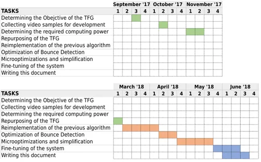
In order to work this project out, it was divided in three phases. The first phase consisting of gathering requirements and specifications from the CAR Institute and refocusing of the project from the original objective to the final one; the second one, were a re-implementation of the original algorithm was done and optimizations were carried out in order to achieve the final objective; and a third one, dedicated to fine-tuning of the system with new material and the writing of this very document.

We now proceed to explain all of the phases, giving a Gannt diagram at the end in figure

2.1graphically showing the timeline of the project.

2.1

First phase

In this first phase, contact was established with the CAR Institute in September of 2017 in order to define the work to be done regarding this project. Given that this project was based on previous year’s work as explained before, the objectives set would be to optimize the algorithm exposed in that work in order to allow processing of the cameras at a high-speed rate and, if possible, implement 3D tracking of the tracked ball.

In order to achieve these objectives, obtaining a couple of high-speed cameras was seen as a necessity in order to implement 3D tracking. For this, CAR offered itself to be the purveyor of such material, tasking themselves with all the logistics of the operation. Once one of the cameras was obtained, a test recording was made in order to gauge the computing power required for the task. To be able to answer the query, we passed the video through last year’s work in order to calculate the performance of it. The computer specifications were then evaluated at requiring a powerful GPU card in order to perform the required computing.

second camera in order to directly implement the system using 3D tracking at a high-speed rate.

At the beginning of March 2018, another meeting was scheduled with CAR in order to have a status report on the second camera only to be met with the fact that it wouldn’t arrive in time for the due date of this project. This meant that 3D tracking would not be possible to implement. Thus, the project pivoted to become only about optimizing as much as possible the given algorithm.

2.2

Second phase

After this reunion, the second step of the project begun. In this, we analyzed the previous algorithm and started its optimization at the same time.

First, we planned on re-implementing the algorithm using a more performant set of tools by first converting the original code to C++ maintaining all of the algorithm steps while replacing some computations with some very simple reworkings that would eliminate unnecessary steps.

Afterwards, work began on bounce detection and implementation of an optimized pro-cessing pipeline for it using linear-algebra libraries.

Finally, some micro-optimizations and algorithm simplifications were carried out in order to accelerate the rate of processing even further.

All of the technologies used in this phase of the project and the final implementation are exposed after this section.

2.3

Third phase

Once all of the implementation steps were carried out, a final meeting was scheduled with CAR. In it, the results of the project were shown. At the same time, several recordings were additionally made in order to fine-tune the pipeline of the project and improve its performance. After this reunion, additional minor modifications were carried out in order to optimize the processing flow and performance metrics.

September '17 October '17 November '17

TASKS 1 2 3 4 1 2 3 4 1 2 3 4

Determining the Obejctive of the TFG Collecting video samples for development Determining the required computing power Repurposing of the TFG

Reimplementation of the previous algorithm Optimization of Bounce Detection

Microoptimizations and simplification Fine-tuning of the system

Writing this document

March '18 April '18 May '18 June '18

TASKS 1 2 3 4 1 2 3 4 1 2 3 4 1 2 3 4

Determining the Obejctive of the TFG Collecting video samples for development Determining the required computing power Repurposing of the TFG

Reimplementation of the previous algorithm Optimization of Bounce Detection

Microoptimizations and simplification Fine-tuning of the system

Writing this document

Chapter 3

System design

In this chapter we present the given system at a high enough level for anyone to under-stand. Additionally, we explain the different technologies used and the reasoning behind it in order to better understand why the system is structured as it is. As a final touch, we also give a diagram of the system architecture for better following of the presented system.

3.1

High level design

In broad strokes, the system takes as input a frame from a camera mounted above the table, processes it using a fine-tuned computer vision pipeline and then outputs a set of coordinates for where the ball is at that time.

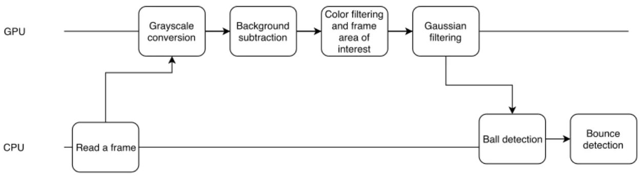
In a bit more specific terms, the system has a high-speed camera mounted 5 meters above the ground in a downward angle at the table. From here we do a bit of preprocessing using the first frame to establish a background to compare against in future frames. Unlike the previous version, the table detection step has been disregarded as it was found to be unnecessary and prone to errors. Afterwards, we consume a frame at a time from the camera and pass it down our pipeline that will use GPU-accelerated computer vision algorithms in order to produce a usable set of elements for later processing. In order to better understand the system we show a diagram in figure 3.1. Each line represents a processor.

In order to understand why there are two processors it helps to visualize the GPU and CPU as separate components that communicate to one another, each having its own memory. The arrows going from CPU to GPU mean an image transfer and the same for the opposite direction. This comes to show how our system can work so fast, it minimizes time spent not doing useful computations. The arrows going from one block in a processor to the next one are steps of the computation.

Read a frame Grayscale conversion Background subtraction Color filtering and frame area of interest Gaussian filtering

Ball detection _detectionBounce GPU

CPU

Figure 3.1: An architectural diagram of the system

3.2

Libraries and technologies

For this project we chose to use OpenCV [1], which is a library containing numerous algorithms of computer vision. In particular, this library has implemented multiple versions of the same algorithms with GPU acceleration. This means that we can use the massively parallel nature of Graphics Processing Units (GPU) and apply it to the image processing world. This allows us to greatly accelerate our processing flow.

To further explain, OpenCV’s implementation of GPU-accelerated computing relies on Nvidia’s CUDA platform, which is a framework created by them in order to expand the use of their GPUs in the High Performance Computing world. This though, forces us to adopt their graphics card exclusively, as it is not usable with other manufacturer’s chips (i.e. AMD).

With this, we had most of our processing flow covered.

One last element required was a linear algebra library in order to solve the required equations for bounce detection. For this we chose to base ourselves around Armadillo [2], a library tailor-made for linear algebra that had a simple interface yet was rated highly in different benchmarks.

In order to bind all of these element together, we needed a fast programming language. Python was discarded as even though it was what it was used previously, it is an inter-preted language instead of a compiled one. This proved to be unusable for our task, as every microsecond not spent processing the image counted against us. For this we chose to use C++ in its modern form with the C++14 standard. This programing language fulfills our requirements of being both fast and expressive, allowing us to use all of the above libraries without incurring programming costs.

3.3

Camera position

To achieve optimal performance we required a camera position from which we could frame the entire playfield. This meant mounting the camera above the table. In this manner we could record all movement without numerous occlusions and distracting background movement.

To be more precise, we mounted the camera 5 meters above the table pointing downwards. To achieve the high-speed condition, we established a framerate of 220 frames per second to be the minimum. Having less than that would imply a loss in precision while tracking the ball.

In order to ease the processing, colour was seen as an important aspect to take into account in order to reduce false positives. This was a balanced trade-off between image quality and valuable data, as the colour allowed filtering for objects with the same colour as the ball.

Chapter 4

Implementation

In order to implement the system, much care has gone into the memory location of the operations. This translates into reducing the amount of time spent transferring data back and forth between the CPU’s and GPU’s memory (Host and Device in CUDA terminology). As a side-effect, this forced us to disregard operations that wouldn’t run on the GPU in intermediate steps between preprocessing and ball detection.

Luckily, the algorithm allows a big chunk of the heavy duty operations to run on GPU exclusively. This translates in a pipeline that given an image as input, will return an easy to process image. The rest of the operations (i.e. detecting the ball and bounce) run on CPU space from then on, as it would be an unnecessary expense of resources to achieve no improvement of performance.

The pipeline will thus be divided in two parts: GPU processing, and CPU processing. With GPU processing being done with OpenCV and CPU processing being done with the aid of both OpenCV and the Armadillo linear algebra library.

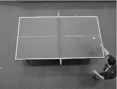
To visualize our operations we will be applying all of them sequentially to the image in figure4.1.

4.1

GPU processing

4.1.1 Preprocessing

As a first step, the image has to be converted to grayscale as seen in figure 4.2. The requirement for grayscale comes due to technical reasons in how the ball object is detected by the CPU algorithm.

Next comes background subtraction as a way to isolate moving objects in the image. For this we use a MOG2 background subtractor. In the original implementation this was

Figure 4.1: The original frame

done with parameters adjusted to a given framerate. Since the framerate has increased by a factor of 5x, these have had to be adjusted to:

Table 4.1: Values of the MOG2 Background Subtractor Parameter Value

History 500 Threshold 16

Shadows? No

The increase in history means that only the last two seconds will be used as history to track. Additionally, the learning rate was left for OpenCV to choose from, as it produces acceptable results and was an easy choice to make.

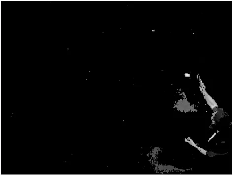
The avid reader might have noticed that in the previous system version there was a table detection step in order to establish table boundaries for later decision making in which ball detection algorithm to apply. This has been removed in this version, as the system was found to be very error prone and produced misguided calls in finding the table. In particular, the table was never found in some cases, which made the whole point of it to be useless. The result of the subtraction can be seen in figure4.3.

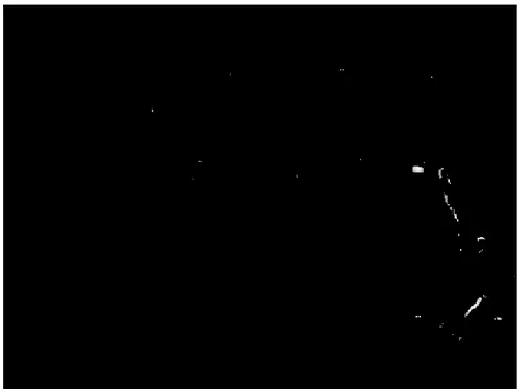
Figure 4.3: Image with only the elements detected by the background subtraction To further aid the selection of what parts of the image we want to observe and reduce false positives, a colour filtering takes place by converting the image to HSV color space.

This is followed by applying two thresholds to the Saturation and Value channels in order to only accept white colours, these can otherwise be modified to process orange, as is the case of tennis table in some places. To use these elements in the code, we simply do a bitwise AND between the resulting thresholds and the background mask. This produces the final desired mask of the image. Applying that to our image we obtain the result in figure4.4.

Figure 4.4: Image after filtering for white elements

The colour conversions are relatively expensive operations that cannot be optimized much more, as they are already being done in GPU.

The applied thresholds in the project for detecting only white elements are: Table 4.2: Threshold values for white colour filtering

Channel Threshold Type Saturation 100 BINARY_INV

Value 150 BINARY

4.1.2 Obtaining area of interest

As was the case with the previous implementation [3:12] we reduce our area of interest to a square centered on the position of the last point location of width and height equal to 60. This number was chosen empirically to reduce the need for computing the optimal

width and height, as that computation wouldn’t achieve any optimization and in fact might slow down the pipeline. In the case we didn’t detect the ball previously, we look in an area 4x times bigger centered on the last seen position. In other words, we double the radius to 120. As such case won’t happen often, the cost is negligible for an increase in robustness.

The reasoning for a square is to allow OpenCV to actually reduce the space to do computations on. On the previous implementation, the author applied a circular mask to the entire image, mistakenly assuming that it would reduce computation time. On the contrary, this did almost nothing to it, given that OpenCV still searched around in the entire, mostly empty, image. By forcing the image down to an area of interest and saving the offset to recompute the correct position, we can do more expensive operations. This is without doubt the most important optimization step of the entire pipeline, transforming the original image into a small 60x60 square.

4.1.3 Post-processing

The post-processing operation is merely an aiding step for the ball detection algorithm that runs on CPU. Namely, we apply a Gaussian filter with a 5x5 kernel to smooth out the image. The result can be seen in figure4.5

4.2

CPU processing

As the image has now been fully processed, we are now ready to transfer it back to the host in order to do the detection itself.

4.2.1 Ball detection

Unlike the previous implementation, the algorithm has been streamlined into a much more simpler one. Previously, one algorithm of two was chosen depending on the ball’s position. This is no longer the case.

In the proposed version we have deemed unnecessary such operation and instead applying OpenCV’s SimpleBlobDetector always, previously used only when out of the table. Three detection options were tested, the two original algorithms (OpenCV’s

Simple-BlobDetector and findContours) and a third one that ran fully on the GPU (Hough Transform). The last one was deemed a failure, as it was actually slower than the CPU

versions by a factor of 3x and had much less precision. findContours was also discarded as it failed when there was more than one object in frame as explained by the previous author [3:13].

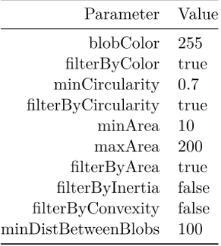
Significant modifications were made to the parameters for the SimpleBlobDetector once the algorithm for it was understood in order to optimize speed and performance. In particular three decisions were made: disable filters activated by the predecessor, enable filtering by size, and reduce the time spent in it by a factor of 2 simply doubling the step size.

The first two decisions were made by realizing that they were being too restrictive. In particular, inertia and convexity weren’t improving actual precision by much yet were being somewhat expensive to operate and tune. This led us to the disabling of them and introduction of filtering by area, a much simpler concept that would filter out big blobs such as sponsorship logos on shirts by players (a common thing in the sport) or wrong things like bright shoes. Note that this parameter should be adjusted in case the resolution of the video changes. Circularity filtering was preserved, as it was a cheap and accurate way of distinguishing circular objects.

The last and most peculiar element was discovered as the algorithm was understood.

SimpleBlobDetector repeatedly applies thresholds to the image in order to isolate blobs

by brightness. The thresholds given by default are very accurate, advancing the threshold in steps of size 10 from 50 to 220. The step size was seen as very small and increased to 20 after looking at the grayscale images of the ball and discovering that most of the time the ball had brightness values bigger than 100, much smaller than 220. This very simple optimization increased performance by 28% in some of our benchmark videos. One more minor note was the minDistBetweenBlobs parameter being used as a dumb

way of merging all blob detections in a radius of 100 pixels so as to minimize detection errors.

Table 4.3: New values for the SimpleBlobDetector

Parameter Value blobColor 255 filterByColor true minCircularity 0.7 filterByCircularity true minArea 10 maxArea 200 filterByArea true filterByInertia false filterByConvexity false minDistBetweenBlobs 100

As a matter of increasing robustness, we added a fallback method that would run

find-Contours if and only if the last detection was made with the SimpleBlobDetector. This

is done on the basis that it would avoid problems where the detection sometimes fails, in which case the cost of doing a cheap operation allows us to avoid increasing the radius of the area of interest in the next frame. This would introduce the possibility of detecting a wrong element as a ball, which would cause problems in future detections.

The final step is to recover the original ball’s coordinates from the area of interest. To do this we use the coordinates of the top leftmost point of the area and add them to the found ball.

4.2.2 Bounce detection

As we have the ball position, we now have to distinguish whether or not there has been a bounce. In order to do this we use the same algorithm as the previous version. In it, we fitted a second degree parabola of form 𝑎𝑥2_{+ 𝑏𝑥 + 𝑐 = 𝑦 with the last four points}

in order to detect a residual error of large enough magnitude, indicating a bounce had ocurred.

The threshold used for this has been maintained at 𝑡 = 0.6. As an observation though, this threshold is unusable for the original videos used for testing purposes. In particular, in those cases, a threshold of 0.2 was found to be accurate unlike the original that had too many false positives. This indicates a particular fragility to angle of camera and possibly even resolution.

Going back to the problem, to optimize this element we were forced to re-implement the algorithm using a linear algebra library. In particular, the library chosen was Ar-madillo [2] due to its simplicity of use and permissive license, allowing it to be exploited commercially if so desired.

The difficulty was overcome by implementing a variation of the algorithm used for fitting a polynomial with an exact fit over the points. In particular, this required the economical QR factorization of the Vandermonde matrix of all four points. The economical version was deemed necessary as the normal QR decomposition wouldn’t work on a non-square matrix (more precisely, it was a 3x4 matrix). The resulting Q and R matrices are then multiplied as 𝑅−1_𝑄𝑡_{𝑦 to obtain the coefficients for the polynomial. This algorithm is}

based on the one shown on Wikipedia’s QR decomposition page [4]

As a last step to calculate the squared residual to see how much the given curve fits the points we calculate the difference between the polynomial at the specified points and the real positions. The result is then squared and summed to obtain the final value to be used in comparison with the threshold.

The process is repeated if a bounce is detected with the three last positions (excluding the newest one as it has already bounced), giving an exact parabola fit. It is then applied to the midpoint between the last detection and the previous one. Assuming that the bounce happened between the last and previous detection. The resulting point (𝑥, 𝑃 (𝑥)) is then assumed to be the bouncing position.

Chapter 5

Results

In order to do a comparison we reused the method in last year’s thesis. In particular, we did these two metrics in addition to the main focus of this project, which is speed:

• Ball detection: A simple check of whether a ball was in the frame or not. • Bounce detection: A simple check on whether a bounce had happened or not

with a margin of error of ±3 frames. The margin was necessary as even during manual labelling it was hard to pinpoint at which frame it had occurred

While we are explaining our results, we will also be comparing them against Christian Soler’s program.

The original program had a filter by blob area that was highly dependent on the input video. As such, to guarantee fairness, the threshold was modified from a minArea of 100 down to 10. This same value is used in our own system, as per the implementation shown above.

5.1

Testing set

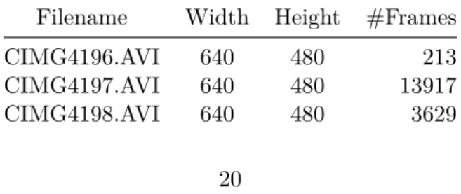
In order to obtain the desired results we revisited CAR in order to gather more video footage. In particular, all of the videos were shot from 5 meters above at a downwards angle pointing at the table, you can see a sample of the videos in figure5.1. The specifics of the videos are as follows:

Table 5.1: Filenames and their respective specifications

Filename Width Height #Frames CIMG4196.AVI 640 480 213 CIMG4197.AVI 640 480 13917 CIMG4198.AVI 640 480 3629

Filename Width Height #Frames CIMG4199.AVI 640 480 3661 CIMG4200.AVI 640 480 3661 CIMG4201.AVI 448 336 8681 CIMG4202.AVI 448 336 8489 CIMG4203.AVI 448 336 9049 CIMG4204.AVI 448 336 7145 CIMG4206.AVI 448 336 8393

Figure 5.1: Sample from the videos

The metrics were obtained via manual labelling of the CAM4201.avi video (total of 8681 frames) due to its appearance of players in the camera and change of lightning conditions. Namely, they forgot we were in the room and started turning lights off.

5.2

Speed of processing

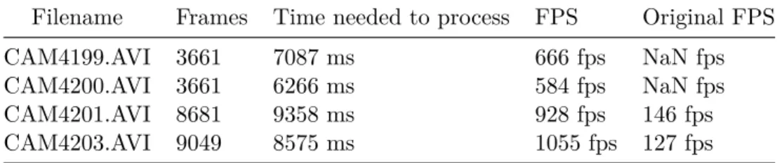
Given that this project was about speed, we ran the program on 4 different file samples given to us by CAR. In order to subtract input/output delays out of the equation, we load the entire video into memory first and then iterate over the frames one by one. This way, we won’t have to take into account decoding the video image and/or reading the file from disk. We compare this also with Christian Soler’s proof-of-concept program in the last column.

Table 5.2: Rate of processing for four different files

Filename Frames Time needed to process FPS Original FPS CAM4199.AVI 3661 7087 ms 666 fps NaN fps CAM4200.AVI 3661 6266 ms 584 fps NaN fps CAM4201.AVI 8681 9358 ms 928 fps 146 fps CAM4203.AVI 9049 8575 ms 1055 fps 127 fps

The objective was to achieve a rate of processing of 300 fps from the original 30-60 fps. The results have more than surpassed that, achieving rates of up to 1,055 fps with the sample videos in colour and a resolution of 448x336. This in turn allows reducing costs in the camera since the required resolution is much lower than HD quality. As we can also see, our implementation beats the original one’s performance by up to 8x.

As can be seen also, the original version failed to even run properly in the first two files due to the table not being found correctly. This is an indicator as to the reasons why we removed this problematic element from our system.

5.3

Timing metrics

In order to understand the time spent per operation we produced a chart that shows each operation in a full run. Full run meaning a frame where a bounce takes place and requires construction of the bounce location.

As can be seen in figure 5.2, around half of the time is spent in the GPU processing stage, with the other half being spent in ball detection. With this info on hand, there is an optimization that could be applied in this case, which is operation pipelining. In the current project however, we didn’t implement this, as we didn’t have enough time. However, the required changes to the code shouldn’t be large enough that they cannot be done without a complete refactoring of it.

Figure 5.2: Time spent per operation in a full run that includes a bounce occurring

Table 5.3: Time spent in each operation

Operation Time spent

Color Conversion 101 𝜇𝑠

Background Subtraction 156 𝜇𝑠 ROI isolation and colour filtering 223 𝜇𝑠

Gaussian filtering 62 𝜇𝑠

Ball detection (CPU) 457 𝜇𝑠 Bounce checking (CPU) 6 𝜇𝑠 Bounce location calculation (CPU) 61 𝜇𝑠

5.4

Ball detection

The tools used for this were in two files (ground truth, and program’s output) that had 8681 lines containing either a p for having a ball, and a q for not having a ball. The bash program used for computing these results can be found in the annex.

Table 5.4: Confusion matrix for ball detection

Predicted \ Actual Actual Ball Present No Ball Present

Ball detected 2689 128

No Ball 553 5311

As we can see, this system has considerable success in detecting the ball with a recall of ~82.9% and a precision of ~95.4% considering the system only degraded its performance

once all the lights went out.

If instead we only filter for the first 8,000 frames (ones with good lighting conditions), we get the following confusion matrix:

Table 5.5: Confusion matrix for ball detection with the first 8,000 frames

Predicted \ Actual Actual Ball Present No Ball Present

Ball detected 2644 128

No Ball 219 5009

Which results in much better results. This would give us a recall of ~92.4% and a precision of 95.4%. Showing us that we have a robust system in place for detecting the ball.

Comparing this against the original version, we obtain the following results with the same first 8,000 frames:

Table 5.6: The confusion matrix for the previous system

Predicted \ Actual Actual Ball Present No Ball Present

Ball detected 2376 293

No Ball 487 4844

As can be seen, the system has a precision of ~89% and a recall of ~83%. These numbers show that our system offers a significant accuracy boost when compared against the original.

5.5

Bounce detection

For bounce detection we repeated the same process as before with two files, except that due to possible errors, we had to code a small utility to calculate the performance for us

with a tunable margin of error. In this case, we assumed a margin of error of 3 frames before or after the bounce happened.

Using the algorithm as it is produced underwhelming results. The confusion table for a margin of error of 3 and a threshold of 0.6 was the following:

Table 5.7: Confusion matrix for the bounce detection Predicted \ Actual Actual Bounce No Bounce Bounce detected 7 98

No Bounce 24 8552

The results are as we said, underwhelming. With a precision rate of ~6.7% and a recall of ~22.6% the system is practically useless for most if not all purposes.

The performance in this case did not improve by tuning the threshold in any meaningful way.

There is a reason why the performance actually worsened compared to the previous version. The reason for that is structural to the algorithm itself and the increase in framerate from the cameras. In the algorithm we take the last 4 detection points in order to gauge whether we had achieved a bounce or not. In order to discern that, we fitted a parabola through those points and calculated the squared error of it. Now, previously those same 4 points were obtained from a much lower framerate camera, producing points that were separated and when discretized, the error wouldn’t affect the parabola much.

When we move the points much closer, as it happens with the new high-speed cameras, discretizing them will introduce a significant error when fitting the parabola and the squared error would cause a lot of false positives since it becomes very susceptible to the discretization step.

All in all, we think that with a bit of work in this regard the algorithm would improve its results a bit, but not as much so as to achieve practical results. Instead, we would focus ourselves on trying to use the ball detection coupled with another camera in order to achieve 3D tracking.

Comparing this to the original version however, we obtain the following: Predicted \ Actual Actual Bounce No Bounce

Bounce detected 0 0

No Bounce 31 8650

The results might come as a surprise, but it is true that no bounce was found according to the previous system. There is a reason for that though which is due to the table

detection step. In the previous version, there was a step that tried to detect the ball in order to apply either one ball detection operation or another. In the given video the table is never found, thus assuming the ball is always out of the table and disregarding those bounces. This comes to show the fragility of failing that first calibration step and is again a reason why we don’t try to find a table.

If instead we disable that check, we get the following results:

Predicted \ Actual Actual Bounce No Bounce Bounce detected 10 61

No Bounce 21 8589

Resulting in a much improved rate of ~14% precision and ~32% recall rates. This, while being a lot better than before and an odd improvement over the proposed system’s performance, still won’t make the detection useful for us as it is too imperfect, failing for the same reasons as explained before.

Chapter 6

Future Work

Even though the presented system works fast and is accurate when it comes to detecting the ball, it still hasn’t solved the bounce detection problem accurately. To this end, we offer the chance of exploring some possibilities.

6.1

3D tracking

Given that the system can work very fast at detecting a ball, we propose using the same system to process multiple cameras at the same time. In this manner, we could very well track a ball in 3D space since we would have the coordinates of the ball in each camera’s viewport and the camera’s position and angle itself.

This easy to say but hard to implement project would quite possibly render our version of bounce detection obsolete. Plus, it would be a very robust system for detecting bounces as the problem would reduce to a change of direction in the height axis.

In addition to solving the bounce detection problem, we could also fix one of the flaws that are to a certain extent hard to solve, namely white elements that look like balls on the players. In this case, the system can act irrationally and track the false ball until it is obstructed again by the player’s movement. This could be fixed by using an ensemble of cameras each detecting the ball individually and then merging their results.

An additional problem one would have to solve is the split-brain problem. In it, we find one camera detecting a ball correctly and another one incorrectly. The question lying in which one is telling the correct answer given our previous tracking history. This problem only accentuates with the addition of multiple cameras for improved tracking.

We say this last point in this section and not another due to the fact it would be an issue to solve in the 3D tracking problem and would make the system much more robust to false positives.

6.2

Tracking multiple balls

Our system is based on the idea of having one and only one ball in frame. With this in mind, suddenly having multiple balls in frame becomes a problem. We don’t know which ball to track. In order to solve this, the program could theoretically be re-purposed to process multiple balls at the same time.

In this manner, one would be able to track multiple trajectories for training purposes. This would also allow faster paced playing, as during our visits to the CAR center, some games had stray balls on the table just because it would eventually roll off the table and was very close to the net, becoming a non-disturbing element of the play.

In particular, this can be of great importance to trainers, as they could for example do a series of fast servings and track all of them without experiencing difficulties.

6.3

Implement efficient pipelining of the operations

Something that has been left to do is implement efficient pipelining of the operations. Given that the operations happen in two stages, one could implement pipelining of the GPU and CPU. In other words, while the CPU is processing one set of instructions, the GPU could be processing the next frame at the same time. Then the CPU would be constantly processing instead of remaining idle for 50% of the time, as the timing metrics showed in figure ??.

This has the potential of doubling the performance, as the effective time spent in a frame would go down to half of the current results.

Chapter 7

Conclusion

In conclusion, the proposed system achieves with remarkable success the established objectives of 200 frames processed per second. What is more, currently the system can process images at up to 1,000 frames per second, much higher than the established objective. This will surely be useful in case of trying to achieve 3D tracking, as we can obtain the ball’s position from multiple cameras at the same time using the same machine without sweating much.

Additionally, the system can work with cameras of considerably low resolution given the ball’s size. The image can even have a somewhat noisy quality due to high ISO value and still work properly, which allows reducing expenses on the camera.

Unfortunately, even though originally supposed to, we couldn’t achieve 3D tracking due to the lack of cameras. With the proof-of-concept though, this can be easily adapted into since it allows the processing from multiple points of view.

We highly encourage further development of the 3D solution basing future works on this system as in our opinion it is the most probable way of achieving a correct bounce detection without false positives and further improvement of the ball detection step.

Appendix A

Proof-of-concept

A.1

Dependencies

The program depends on the following:

• OpenCV 3.4.1 being compiled with CUDA 9.0+ • Armadillo 8.400+

• cxxopt for options handling

These are the only three dependencies the program has, cxxopt is already included in the project in the form of a headers only library.

A.2

Format of output

By default the program outputs the detections to stdout in the format x,y,timestamp where x and y are coordinates of the video. If there is no ball in the frame, the system will print -1,-1,<tstamp> so as to show that there was no ball.

The same applies to the bounces, except there we only print the bounce instead of both bounces and non-bounces.

A.3

Options

The program has some useful options listed here:

• -i,--input: The given input video file to process (uses OpenCV, so it allows any video file to be used)

• -v,--video: Will output an H.264 video file with a visualization of the output. Green dots and lines represent a ball trajectory while larger blue dots represent a bounce. By default we don’t have

• -b,--bounces-out: A path to where the bounces will be printed to. By default it won’t print anywhere the bounces.

• -d,--detections-out: A path to where the detections will be printed out, by default it will print to stdout.

Appendix B

Performance calculators

Here we give the programs used to calculate the performance of the systems.

B.1

Detection

The two files were processed with the simple bash one-liner: paste -d "" ground_truth.txt out.txt | \

awk '

/qq/ { a["trueneg"] += 1 } /pp/ { a["truepos"] += 1 } /pq/ { a["falseneg"] += 1 } /qp/ { a["falsepos"] += 1 }

END { for (key in a) { print key, a[key] } }'

B.2

Bounce

To do this we had to create a simple Python program that would know to analyze the outputs with a given radius.

import argparse

from typing import List

def bounce_in_gt(ground_truth: List[str], bounce_pos: int, radius: int = 1) -> bool: return 'b' in ground_truth[max(bounce_pos - radius, 0) : bounce_pos + radius + 1] def main():

parser.add_argument("ground_truth", type=argparse.FileType()) parser.add_argument("out_file", type=argparse.FileType()) parser.add_argument("-r", "--radius",

help="Allowed margin of error for bounce detection", type=int,

default=3

)

args = parser.parse_args()

ground_truth = ''.join(x[:-1] for x in args.ground_truth) false_pos = 0

true_pos = 0

for i, detection in enumerate(args.out_file): if 'b' in detection:

if bounce_in_gt(ground_truth, i, radius=args.radius): f = ground_truth.find(

'b', max(i - args.radius, 0), i + args.radius + 1

)

ground_truth = ground_truth[:f] + 'q' + ground_truth[f+1:] true_pos += 1

else:

false_pos += 1

false_neg = ground_truth.count('b')

true_neg = len(ground_truth) - false_neg - true_pos - false_pos print("truepos", true_pos) print("falsepos", false_pos) print("falseneg", false_neg) print("trueneg", true_neg) if __name__ == "__main__": main()

B.3

Timings

We modified the program to output microsecond timings of all the operations in the form of <conversion> <subtraction> ... and used the following awk script to parse

the file: awk '{ a["conversion"] += 1; b["conversion"] += $1; a["subtraction"] += 1; b["subtraction"] += $2; a["isolation"] += 1; b["isolation"] += $3; a["filtering"] += 1; b["filtering"] += $4; a["detection"] += 1; b["detection"] += $5; if ($6 > -1) { a["bounceCheck"] += 1; b["bounceCheck"] += $6; } if ($7 > -1) { a["bounceCalculation"] += 1; b["bounceCalculation"] += $7; } }

References

[1] G. Bradski. 2000. The OpenCV Library. Dr. Dobb’s Journal of Software Tools (2000).

[2] Conrad Sanderson. 2010. Armadillo: An Open Source C++ Linear Algebra Library

for Fast Prototyping and Computationally Intensive Experiments. NICTA. Retrieved

from http://arma.sourceforge.net/

[3] Christian Jose Soler. 2017. Table tennis ball tracking and bounce calculation using

opencv. Retrieved fromhttp://hdl.handle.net/2445/119897

[4] Wikipedia contributors. 2018. QR decomposition. Retrieved from https: //en.wikipedia.org/wiki/QR_decomposition#Using_for_solution_to_linear_inverse_

problems

[5] Xiao Xiao, Michael S. Bernstein, Lining Yao, David Lakatos, Lauren Gust, Kojo Acquah, and Hiroshi Ishii. 2011. PingPong++: Community customization in games and entertainment. (November 2011), 24.