BIVARIATE VALUE-AT-RISK Giuseppe Arbia
1. MOTIVATION
In its earlier stage of development the theory of financial risk management and portfolio selection was based on simple statistical measures of dispersion of the expected return (such as variance or coefficient of variation) as measures of the global risk of an asset or of the entire portfolio. Similarly the linear regression coefficientβ of an asset, which measures the relative increase in portfolio risk due to an additional unitary investment in that asset, was considered a good measure of the market risk of that asset not due to general market fluctuation and hence a tool to assist the choice in building efficiently diversified portfolios.
It is now widely accepted that the variance of the expected returns measures a rather inaccurate notion of risk due to the frequent asymmetries and fat tails displayed by the asset’s returns distributions (Afflect-Groves and McDonald, 1989). The concept of value-at-risk (VaR) has taken place as the new benchmark in the risk management techniques that takes downside risk into account (Jorion, 1997).
The VaR approach is based on a general (long known) notion of risk as the probability of exceeding (or not exceeding) a certain cut-off quantity perceived as dangerous. Such a definition is by no mean peculiar to finance and has found applications in many different fields such as insurance (Williams and Heins, 1976), technology (Hultzer et al., 1983), environmental analysis (Simmons et al., 1973), engeneering (Diamond, 1981) and many others (for a review see e. g. RSS, 1999).
Specifically, financial risk can be viewed as the probability of not exceeding a cut-off return (say R*) on a random distribution (Cramer, 1930). Such a distri-bution can be an explicit random distridistri-bution, characterized by say, a density functionf (r)R , thus leading to a parametric (or model dependent) approach to
VaR, or, alternatively, an implicit distribution based on the historical empirical distribution of returns (or model-free, see Artzner et al., 1998).
At a given cut-off point R* the risk can be evaluated as: Risk f u duR F RR R = = −∞
∫
( ) ( *) * = 1 - α (1)with F RR( )* the cumulative distribution function of the asset returns distribu-tion evaluated in the point R*. Conversely, at a maximum accepted level of risk 1–α (e.g. α = 0.99 as required by the Basle Committee on Banking Supervision, 1996), the cut-off return is found by solving equation (1) with respect to R. If we call R( )α such a solution, the VaR of a unitary investment is then evaluated as
VaR( )α = −R( )α
For reasons that will become clearer in the remainder of the paper we will henceforth refer to −R( )α as the Uni-VaR of an asset or of the entire portfolio.
The general definition of risk given in (1) is very intuitive and encompasses the traditional measure of variance as a special case when the asset returns are gaus-sian.
In fact, when the expected returns are normally distributed we have
Risk= F rR = − u− du −∞
∫
( *) 1 2 exp 1 2 2 R * πσ µ σ (2)with µ = E(R ) and σ2 = Var(R). Approximations for (2) are given e.g. in
Abramoviz and Stegun (1965).
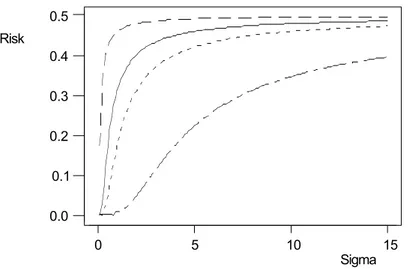
Figure 1 shows the plot of the risk as measured in equation (1), against the standard deviation for various values of the cut-off return expressed in standard-ized scores ranging from -4 to -0.5.
Figure 1 shows that in the normal case the general risk measure of equation (1) is a monotonically increasing function of σ. Although the function is non-linear, the choice between the two measures does not affect the ranking of risk, and this implicitly justifies the use of the standard deviation in past decades as a proxy to risk when empirical distributions do not depart dramatically from normality.
With the introduction of the VaR techniques it is recognised the crucial role of non-normal returns placing a greater emphasis on the left tail of the returns’ distributions. This produces more accurate estimate leading to tremendous impli-cations in terms of risk management, evaluation and ranking.
In this paper we claim that it is possible to extend the idea of VaR to “market risk” evaluation and portfolio management giving the right consideration to downside risk exposure.
The set up of the paper is the following. In the next section we will consider a general definition of market risk of an asset based on definition (1) that admits the traditional β measure as a particular case when returns are normal. The data used and the results are presented in section 3. Section 4 contains some conclu-sions and directions for further studies in the field.
0 5 10 15 0.0 0.1 0.2 0.3 0.4 0.5 Sigma Risk
Figure 1 – Plot of the global risk measure of equation (1) as a function of the standard deviation of
the returns for various values of the cut-off return expressed in standardized scores. Lower line refers to -4. Upper line corresponds to -0.5 The solid line considers a probability of 0.99 corresponding to the Basle requirement.
2. VALUE-AT-RISK IN A BIVARIATE CONTEXT
Let us consider a portfolio P characterised by a random return Rp with expected
value E(Rp)= µp and variance Var(Rp) = σP
2
. Suppose now that we want to evalu-ate the market risk of introducing in this portfolio a new unitary investment in, say, asset-1.
We will define the market risk of asset-1 as the probability that the new in-vestment does not exceed a certain cut-off (R*1) and simultaneously the portfolio
as a whole does not exceed a certain cut-off (Rp*). This is evaluated through the
integral
Market risk fR R u v dudv F R
R R R R p p p p − = = −∞ −∞
∫
∫
1 1 1 1 ( , ) ( ) * * * * R (3)with FR Rp 1(R Rp* 1*) denoting the cumulative joint distribution function of the asset’s returns and portfolio returns.
Remark 1. If the two random variables associated with the return of asset-1 and
the return of the portfolio as a whole are jointly normally distributed, then defi-nition (3) yields:
Market risk u v u v dudv p R R p p p p p − = − ⋅ ⋅ − −
(
)
− + − − − − −∞ −∞∫
∫
1 2 1 1 2 1 2 1 2 2 2 1 1 2 1 1 * * πσ σ ρ ρ µ σ µ σ ρ µ σ µ σ 1 expwithµp = E(Rp);σp 2 = Var(Rp); µ1 = E(R1) and σ 12 = Var(R1).
Let us now assume without loss of generality that E(Rp) = E(R1) = 0 and, just
for the purpose of illustration, σ1 =σp= 1 and hence: β=Cov( , )1 Cov( , ) 1 1 R R R R p p p σ σ = =ρ. It follows that:
Market risk u v uv dudv
R R p − = − −
(
−)
[
+ −]
−∞ −∞∫
∫
1 2 1 1 2 1 2 2 2 * * π β exp β β 1 2 2Let us now set
w = R − Rp − 1* * 2 1 β β and hence R1* =w 1−β2 +βRp* we have Market risk w v dwdv R w Rp p − = −
[
+]
−∞ −∞ − +∫
∫
21 exp 1 2 * 2 * 1 2 2 π β β = 1 2 exp 1 2 1 2 1 2 2 1 2 * 2 * π π β β − − −∞ −∞ − +∫
∫
w v dwdv R w Rp p ==
1 2 exp 1 2 2 1 2 * π β β − −∞ − +∫
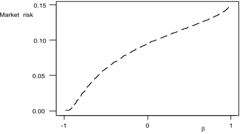
w FR Rp w R p p ( )*Remark 2. Figure 2 plots the market risk associated with asset-1 as a function of
β, showing that in the particular case examined the systematic risk of asset-1 is a monotonically increasing function of the β of the asset itself. This justifies the use of the traditional β of an asset as a proxy for the market risk of the asset itself, if the expected returns are jointly normally distributed.
However equation (3) provides a more accurate tool to justify the inclusion of an asset in the portfolio when the joint distribution departs dramatically from the bivariate gaussian case, as it is the case in most empirical situations. Obviously the joint distribution function can be fully specified or just evaluated non-parametrically from historical record counting.
Remark 3. If the expected returns distribution of asset-1 and the portfolio
re-turn distribution are stochastically independent than the joint distribution fac-torizes as: 1 0 -1 0.15 0.10 0.05 0.00 β Market risk
Figure 2 – Plot of the market risk measure of Equation 3 as a function of the β of the asset
consid-ering a cut-off return of - 0.5 (expressed in standardized scores) for both the portfolio and asset.
fR Rp 1(u v)= fRp( )u fR1( )v and hence Market risk fR u du fR v dv R R p p − = −∞ −∞
∫
∫
( ) ( ) * * 1 1 (4) so that market risk is simply the product of the risk evaluated through (1) for the asset-1 and for the entire portfolio. In this instance substituting (1) into (4) yields:Market risk− = −(1
α
)2 (5)Now let us revert the argument and assign (1−
α
)2 as the maximum level of accepted market risk in Equation (3). If we substitute the cut-off return for the entire portfolio derived from the Uni-VaR technique (R(α
)p) at the level of risk(1−α), we can solve Equation (3) with respect to R1* and obtain the solution R(
α
)β,1such that R( )α
β,1 : fR R u v dudv R R p p 1 2 ( , ) 1-( ) ( ) ,1 −∞ −∞∫
∫
=( )
α α β α (6)We finally define the Bivariate Value-at-Risk (or β-VaR) of an asset as:
β- VaR( )α = −R( )α β,1 (7)
Since at a given probability (1−
α
)2 market risk increases as −R( )α β,1 in-creases, then the β- VaR( )α of an asset is a measure of the market risk of the asset itself.Thus β- VaR( )α is the negative of the (1−
α
)2 quantile of the bivariate dis-tribution of returns having fixed to R(α
)p the (1−α) univariate quantile for theentire portfolio.
Remark 4. The bivariate Value-at-Risk is equivalent to a conditional Uni-VaR
given the portfolio returns’ distribution. In fact
fR Rp u v fR R v u fR u
p p
1( , )= 1 ( ) ( )
and, integrating both sides of the equation with respect to u and v we obtain:
f
R Ru v dudv
f
v u
R dv f
u du
R R R R p R R R p p p p p 1 1 1 1( , )
(
)
( )
-- - -* * * * ∞ ∞∫
∞ ∞∫
=
∫
≤
*∫
If we set Rp* to the level of R(
α
)p corresponding to the Uni-VaR, andfur-thermore the market risk to the level (1−
α
)2 we obtain:1
1−
(
)
=
≤
∞∫
α
f
R Rv u
R
α
pdv
R p(
( ) )
-1*and solving with respect to R1* we obtain again the solution R( )α β,1. Thus the β
-VaR can also be viewed as the negative of the (1−α) conditional quantile (Bas-sett and Könker, 1982) of the returns’ distribution given that the portfolio return exceeds its cut-off point R*.
From a comparison between the β-VaR and the Uni-VaR we can also derive a measure of dependence between the asset’s returns and the portfolio returns. In fact when the portfolio returns and the asset-1 returns are independent then
β- VaR( ) Uni VaR( )α = − α
In the case of positive dependence, however, when points tend to concentrate in the first and third quadrant, the term R( )α 1 is greater than R( )α β,1 and hence Uni-VaR is smaller than β-VaR. Conversely in the case of negative dependence when points are concentrated in the second and fourth quadrants the term R( )α 1
is smaller than R( )α β,1 and hence Uni-VaR is greater than β-VaR.
3. BIVARIATE VALUE-AT-RISK AND NEW MEASURES OF RISK AND MARKET DEPENDENCE
We now make use of the general concept of the positive quadrant dependence (Joe, 1997) measure between two random variables. Two random variables X1
and X2 are positive quadrant dependent if
P X
[
1 ≤x X1; 2 ≤x2]
≥P X[
1 ≤x P X1] [ 2≤x2]
In the case of positive dependency
fR R (u, v)dudv ( ) ( ) p 1 ,1 −∞ −∞
∫
∫
R Rα β α p − ≥ −∞ −∞∫
∫
f (u)duR f (v)dv 0R ( ) ( ) p 1 1 p R Rα αSince at a given α risk and cut-off returns are inversely related, in case of posi-tive dependence
R( ) - ( )α 1 R α β,1 ≥ 0
Thus the quantity
ξ α( )=
[
βVaR( ) UniVaR( )α − α]
≥0 (8) is a general measure of non-linear dependence between R1 and Rp restricted to theleft tails of their joint distribution.
A further measure of market risk can be obtained by computing the expected returns of an asset when these returns do not exceed R( )α β,1
S( )α β,1 =E(R R1 1 ≤R( )α β,1) (9)
This measure is the bivariate counter part of the measure suggested by Artzner
4. DATA ANALYSIS
For the purpose of illustrating the methodology of bivariate Value-at-Risk in the present section we consider a set of Italian stock market data collected daily in the period ranging from the 14th of October 1994 to the 18th of August of 1998. The data set refers to a 960-day long time series of the general Milan stock market index (MIB - Milano Indice Borsa) and to six sectorial indices referring to assets classified as Industrial, Financial, Communications, Credit, Insurance and “Diverse”.
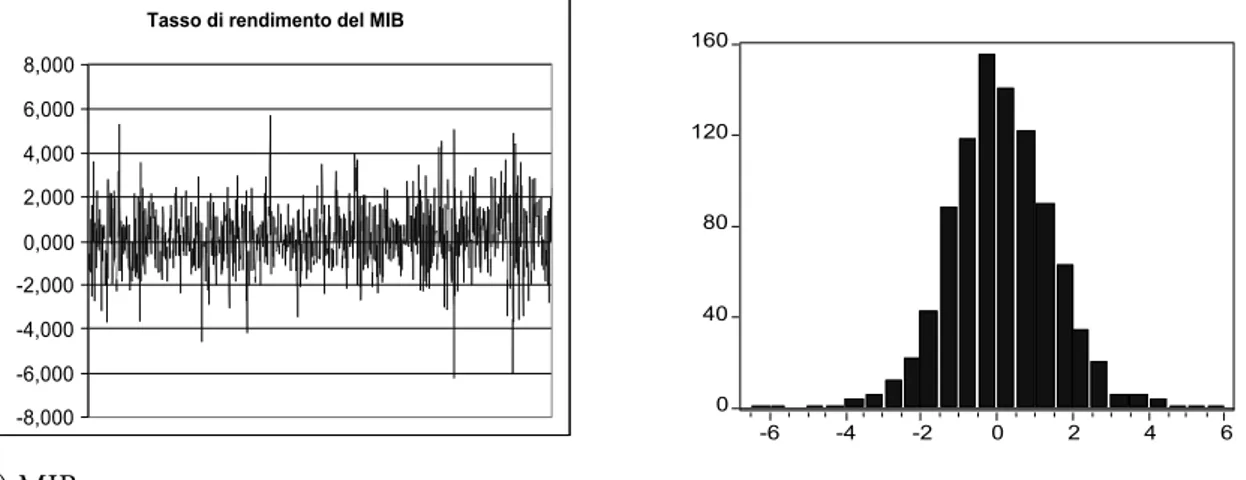
The 7 time series of returns are reported in figure 3 together with the corre-sponding histogram. All series display a market excess kurtosis and a negative skewness (with the exception of the “Insurance” series showing a positive skew-ness and of the MIB series showing no significant skewness).
Table 1 reports the comparison between two global risk measures: the standard deviation and the univariate Value-at-Risk (the traditional VaR), together with the different rankings deriving from the two measures. The value of α =0.95 has been chosen with respect to the length of the time series.
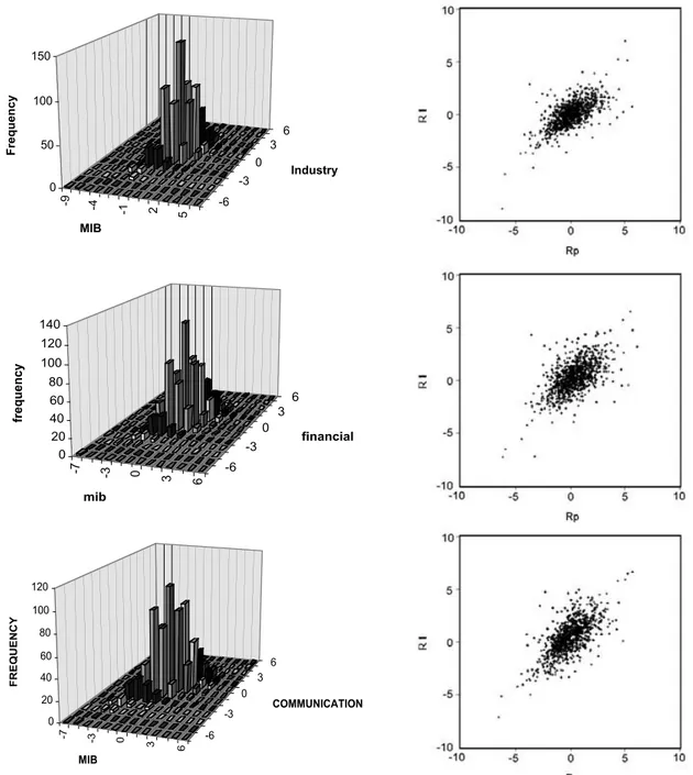
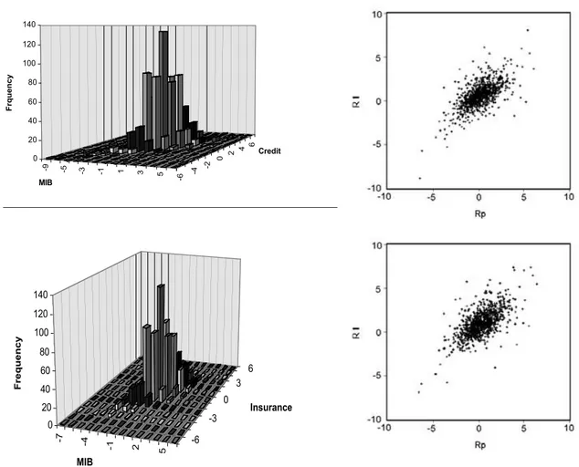
Figure 4 shows the joint distributions of each sector’s return and of the MIB index in terms of a 3-dimensional frequency distribution, and in terms of a scatter diagram. All graphs provide evidence of a positive dependence between all secto-rial indices and the MIB index.
Table 2 compares the traditional β measure with the β-VaR obtained through Equation (7) with α = 0.95, estimated as the quantile of the historical records distributions, making no distributional assumption. Table 2 also reports the non-linear dependency measure ξ(α) suggested in Equation (8). For most sectors the dependency in the left tail is positive; however, for the case of indices referring to “Insurance”, “Finance” and “Diverse” assets, the ξ(α) measure reveals a negative dependence. Finally table 2 reports the two different rankings of risk derived by using the traditional β measure and the β-VaR.
Tasso di rendimento del MIB
-8,000 -6,000 -4,000 -2,000 0,000 2,000 4,000 6,000 8,000 0 40 80 120 160 -6 -4 -2 0 2 4 6 a) MIB
Figure 3 – Time series of the MIB Index (series a) and of the returns of the various assets classified
within 6 categories (series b to g) in the time period ranging from the 14th October 1994 to the 18th August 1998. (continued)
Figure 3 – (continued)
Tasso di rendimento del settore industria
-10 -8 -6 -4 -2 0 2 4 6 8 0 0 0 0 0 -8 -6 -4 -2 0 2 4 6 b) Industrial Financial -8 -6 -4 -2 0 2 4 6 8 0 40 80 120 160 -6 -4 -2 0 2 4 6 c) Financial
Tasso di rendimento del settore delle comunicazioni
-8 -6 -4 -2 0 2 4 6 8 0 20 40 60 80 100 120 140 -6 -4 -2 0 2 4 6 d) Communications
Figure 3 – (continued)
Tasso di rendimento del settore bancario
-9 -7 -5 -3 -1 1 3 5 7 0 50 100 150 200 -8 -6 -4 -2 0 2 4 6 e) Credit
Tasso di rendimento del settore assicurativo
-8 -6 -4 -2 0 2 4 6 8 0 50 100 150 200 -6 -4 -2 0 2 4 6 f) Insurance
Tasso di rendimento del settore diversi
-20 -15 -10 -5 0 5 10 15 20 0 50 100 150 200 250 300 -15 -10 -5 0 5 10 15 g) Diverse TABLE 1
Measures of global risk (σ and Uni-VaR) and relative rankings within parentheses.
σ Uni-VaR(α) Communications 1.568412 (1°) 2.566 (1°) Credit 1.338803 (6°) 1.905 (5°) Diverse 1.487575 (2°) 1.566 (7°) Financial 1.422402 (3°) 2.198 (2°) Industry 1.206565 (7°) 1.828 (6°) Insurance 1.374296 (5°) 1.931 (4°) MIB 1.414148 (4°) 2.051 (3°) Note:α = 0.95
TABLE 2
Measures of market risk: β, β-VaR(α), (and relative rankings within parentheses), Uni-VaR(α) and ξ(α) non-linear tail dependency measure.
β β-VaR(α) Uni-VaR(α) ξ(α) MIB - - 2.051 -Industry 0.5698 (5°) 1.898 (4°) 1.828 0.070 Financial 0.6101 (4°) 2.084 (2°) 2.198 - 0.114 Communications 0.7639 (1°) 2.658 (1°) 2.566 0.092 Credit 0.6264 (3°) 1.943 (3°) 1.905 0.038 Insurance 0.6289 (2*) 1.848 (5°) 1.931 - 0.083 Diverse 0.3813 (6°) 1.080 (6°) 1.566 - 0.486 Note:α = 0.95 -9 -4 -1 2 5 -6 -3 0 3 6 0 50 100 150 Fr eq ue nc y MIB Industry -7 -3 0 3 6 -6 -3 0 3 6 0 20 40 60 80 100 120 140 fre qu en cy mib financial -7 -3 0 3 6 -6 -3 0 3 6 0 20 40 60 80 100 120 FR EQ U EN C Y MIB COMMUNICATION
Figure 4 – Joint distributions of each sectors’ returns and MIB returns (14th October 1994 - 18th
Figure 4 – (continued) -9 -5 -3 -1 1 3 5 -6 -4 -2 0 2 4 6 0 20 40 60 80 100 120 140 Frq uen cy MIB Credit -7 -4 -1 2 5 -6 -3 0 3 6 0 20 40 60 80 100 120 140 Fr eq ue nc y MIB Insurance
Apart from the “Communications” sector, which appears to be the more ex-posed to market risk in both cases, by focusing on the left-tail behaviour of the return, we obtain two remarkably different rankings. In particular the “Insurance” sector appears the least risky with the β-VaR criterion, whereas it is in the second position according to the β criterion. This is due to the negative dependency with MIB in the left tails shown in table 2 and to the positive skewness observed above. Conversely “Financial” and “Industrial” assets appear to be more exposed to market risk if evaluated through the β-VaR than through β. Table 3 reports the ranking of risk obtained by employing the restricted expected shortfall. The ranking obtained is not substantially different from that reported in Table 2 based on the β-VaR.
In order to investigate the dynamics of market risk in the period examined we divided the time series into two subsamples referring to years 1994 to 1996 on one side, and to years 1997 and 1998 on the other (see table 4 and 5). The two sample periods contain a different number of observations, but this has negligible influence on our analysis. The second subperiod includes a period of greater volatility of all indices (see figures 3) due to the instability of stock markets regis-tered in the summer of 1998. In the first subperiod the ranking obtained with the two measures is not very different with “Communications” and “Financial” assets
by far at the top, followed by the other sectors that do not display significant differences in risk. In contrast in the second subperiod “Communications” is followed by “Credit” if we rely on the β criterion, and by “Insurance” if we adopt the β-VaR role. The entire ranking appears to be very different in the two cases. If we compare this evidence with that of table 2, it appears that the differences in ranking of the two measures are greater in periods of greater instability.
TABLE 3
Rank of the restricted expected shortfall of the various asset categories for returns above the β-VaR Sα β
( )
,1 Communications 3.6792 Financial 3.3957 Credit 3.4121 Insurance 3.2685 Industry 3.1611 Diverse 2.3671 TABLE 4Measures of market risk in two subperiods.
10.14.1994 - 12.31.1996 1.2.1997 - 8.18.1998 β β-VaR(α) ξ(α) β β-VaR(α) ξ(α) Industry 0.5370 1.7746 0.0017 0.5959 2.4119 0.1512 Financial 0.6001 1.9379 0.0007 0.6138 2.8908 0.0229 Communications 0.8084 2.4954 0.0228 0.7268 2.9245 0.0168 Credit 0.5715 1.7794 0.0066 0.6647 2.4585 0.2251 Insurance 0.5836 1.6952 0.0045 0.6609 2.8989 0.0388 Diverse 0.3961 1.3555 0.0021 0.3470 1.5356 - 0.0154 TABLE 5
Ranking of assets category according to the two market risk measures in the two subperiods considered
FIRST SUBPERIOD (10.14.1994 - 12.31.1996) β β-VaR(α) Communications 0.8084 Communications 2.4954 Financial 0.6001 Financial 1.93791 Insurance 0.5836 Credit 1.77944 Credit 0.5715 Industry 1.7746 Industry 0.537 Insurance 1.69519 Diverse 0.3961 Diverse 1.35556 Note:α = 0.95 SECOND SUBPERIOD (1.2.1997 - 8.18.1998) β β-VaR(α) Communications 0.7268 Communications 2.9245 Credit 0.6647 Insurance 2.8989 Insurance 0.6609 Financial 2.8908 Financial 0.6138 Credit 2.4585 Industry 0.5959 Industry 2.4119 Diverse 0.3470 Diverse 1.5356 Note:α = 0.95
5. CONCLUSIONS AND DIRECTIONS FOR FURTHER RESEARCH
The aim of this paper is to define measures to properly rank financial risks when the return distributions are not Gaussian and present heavy tails and are skewed. Such measures are needed to emphasize downside risk exposure, which is the main feature to look at in optimal asset allocation and portfolio management. To achieve this aim we extend the VaR measure proposed for global risk evalua-tion to market risk evaluaevalua-tion by introducing the concept of bivariate Value-at-Risk (β-VaR). The method introduced is applied to daily time series of Italian stock market data in the period from 9.94 to 8.98. By using the proposed meth-odology as opposed to the traditional criterion based on the popular linear regres-sion coefficient β, we show that we end up with a very different market risk evaluation and hence with a very different ranking of the assets with respect to risk. We also show that the difference in the two measures is particularly dramatic in a period of higher volatility and market instability like that experienced in the summer of 1998 due to the stock market world crisis.
The work reported here is preliminary and requires further investigation and extensions in various directions.
First of all, in the present paper we did not consider the sampling distribution of the bivariate Value-at-risk. Further work in this area should rely upon the well known results on the inference on conditional quantiles (see e. g. Bassett and Könker, 1982; Steinhorst and Bowden, 1977 and Kabe, 1976) and on the litera-ture about order statistics related to the L-estimators (Sarhan and Greenberg, 1962; David, 1981). The work on bootstrap interval estimation for quantiles by Efron (1981) should also provide a theoretical basis for further work.
Secondly, here we only consider a particular specification of non-linear de-pendence in the left tails of the bivariate distributions of returns. Various alterna-tives that can prove useful in this field (e. g., left tail dependence or general bivariate tail dependence) can be found in the literature on multivariate extreme order statistics (Galambos, 1987; Deuhauvels, 1983, Joe, 1994). For a recent review see Joe (1997). For application to finance see Embrechts et al. (1998).
A third area that deserves special attention is linked to the idea of combining past records and simulation techniques to create worst-case scenarios of market risk through autoregressive conditional models, as indicated in Barone-Adesi et al. (1998) for the standard univariate Value-at-Risk measure, and by Koul and Saleh (1995) in a more general setting. The work on quantile regression (Hogg, 1975; Griffith and Willcox, 1978; Stone, 1977; Casady and Cryer, 1976; and for an application to economic data Buchinski, 1995) and the work of Rousseeuw and Hubert (1999) on conditional median modelling could also be of use in this field.
Finally, in the present paper we propose a measure of market risk referring to a unitary investment of each asset individually taken. A natural extension of the method described here seems to be the derivation of a multivariate VaR for the entire portfolio that takes into account the proportion of investment for each asset within the portfolio. The results on multivariate quantile estimation (de Haan and Huang, 1995) and the general measures of dependence between order
statistics in a multivariate context, like the orthant dependency concept (Joe, 1997), should prove helpful in this field.
Department of Sciences,
University “G. d’Annunzio”, Chieti
GIUSEPPE ARBIA
ACKNOWLEDGEMENTS
I wish to acknowledge the comments and suggestions received by Giovanni Barone-Adesi of Ingano University during many stimulating conversations, those by Dan Griffith of Syracusa University and those by the anonymous referees that improved the first version of the paper. I also acknowledge the comments received by the participants to the Finance Seminar at USI Lugano in June 1999 and by those attending the Royal Statistical Society Conference held in Warwick University in July 1999, where previous versions of this paper were presented.
REFERENCES
M. ABRAMOVITZ, I. A. STEGUN (1965), Handbook of mathematical functions, Dover Publ, NY. J. AFFLECT-GRAVES, B. MCDONALD (1989), Nonnormalities and tests of asset pricing theories,
“Journal of Finance”, 44, pp. 889-908.
Y. AIT-SAHALIA, A. LO (1996), Non parametric estimation of state price densities implicit in
financial asset prices, WP, LFE, pp. 1015-96, MIT
P. ALBRECHT (1999), Normal and lognormal shortfall risk, “Proceedings of the third AFIR
International Colloquium”, Rome, Vol. 2, pp. 417-430.
P. ARTZNER, F. DELBAEN, J-M. EBER AND D. HEATH (1999), Coherent measures of risk,
“Mathe-matical Finance”.
G. BARONE ADESI, F. BOURGOING, K. GIANNOPOULOS (1998), Don’t look back, “Risk”, August,
pp. 100-103.
BASLE COMMITTEE ON BANKING SUPERVISION (1996), Amendments to the capital accord to
incorporate market risk, Basle, January.
G. BASSETT JR, R. KÖNKER (1982), An empirical quantile function for linear models with iid
errors, “Journal of the American Statistical Association”, 77, pp. 407-415.
F. BASSI, P. EMBRECHTS. AND M. KAFETZAKI (1999), Risk management and quantile estimation, in
“Practical guide to heavy tails”, R. Adler, R. Feldman and M. Taqqu, M (eds.), Birk-häuser, Boston.
A.K. BERA, C. M. JARQUE (1982), Model specification tests: a simultaneous approach, “Journal of
Econometrics”, 20, pp. 59-82.
R. BLATTBERG, N. GONEDES (1974), A comparison of stable and student distributions as
statistical models for stock prices “Journal of Business”, 47, pp. 244-280.
M. BUCHINSKI (1995), Quantile regression, Box-Cox transformation model, and the U. S. wage
structure 1963-1983, “Journal of econometrics”, 65, pp. 109-154.
R.J. CASADY, J. D. CRYER (1976), Monotone percentile regression, “Annals of statistics”, 4, pp.
532-541.
H. CRAMÉR (1930), On the mathematical theory of risk, “Festskrift Skand”. 19855-1930.
Stockholm, Sweden.
L. DE HAAN, X. HUANG (1995), Large quantile estimation in a multivariate setting, “Journal of
Multivariate Analysis”, 53, pp. 247-263.
P. DEUHEUVELS (1983), Point processes and multivariate extreme values, “Journal of
Multi-variate Analysis”, 13, pp. 257-272.
W.J. DIAMOND (1981), Practical experiment design for engineers and scientists, Lifetime
Learning, Belmont, CA.
B. EFRON (1981), Censored data and the bootstrap, “Journal of American Statistical
Associa-tion”, 76, pp. 312-319.
P. EMBRECHTS, A. MCNEIL, D. STRAUMANN (1998), Correlation and dependency in risk
manage-ment: properties and pitfalls,ETHZ papers, November.
J. GALAMBOS (1987), The asymptotic theory of extreme order statistics, 2nd edition, Kreiger
Publisher, C. O. Melebar, FL.
D. GRIFFITH, M. WILLCOX (1978), Percentile regression a parametric approach, “Journal of
American Statistical Association”, 73, pp. 496-498.
R.V. HOGG (1975), Estimates of percentile regression lines using salary data, “Journal of
American Statistical Association”, 70, 56-59.
W.P. HULTZER, J. R. NELSON, R. Y. PEI, C. M. FRANCISCO (1983), Non-nuclear Air to Surface
ordinance for the future: An approach to propulsion technology risk assessment,RAND
Corp., Santa Monica, CA.
H. JOE (1994), Multivariate extreme value distributions with applications to environmental
data, “Canadian Journal of Statistics”, 22, pp. 47-64.
H. JOE (1997), Multivariate models and dependence concepts, Chapman and Hall, London. P. JORION (1997), Value-at-Risk: The new benchmark for controlling derivatives risk.
McGraw-Hill.
D.G. KABE (1976), On confidence bands for quantiles of a normal population, “Journal of
American Statistical Association”, 71, pp. 417-419.
H. KOUL, A. K. SALEH, E. MD (1995), Autoregressive quantiles and related rank-score processes,
“Annals of statistics”, 23, pp. 670-689.
N. PAPADATOS (1995), Methods to approximate joint uncertainty and variability in risk, “Risk
Analysis”, 15, pp. 411-419.
P.J. ROUSSEEUW, M. HUBERT (1999), Regression depth, “Journal of the American Statistical
Association”, 94, pp. 388-402.
RSS (1999), Royal Statistical Society Conference Abstracts. Theme: risk, July 1999,
University of Warwick.
A. E. SARAHAN, B. G. GREENBERG (1962), Discriminant confidence bands on percentiles, Eds
Contributions to order statistics, Wiley, NY.
J.A. SIMMONS, R. C. ERDMAN, B. N. NAFT (1973), The risk of catastrophic spills of toxic chemical, NTIS, Sprinfield, VA.
C.J. STONE (1977), Consistent non parametric regression, “Annals of statistics”, 5, 595-645. R.K. STEINHORST, D. C. BOWDEN (1977), Discrimination and confidence bands on percentiles,
“Journal of American Statistical Association”, 66, pp. 851-854.
G.A. WILLIAMS, R. M. HEINS (1976), Risk management and insurance, 3rd ed. McGraw-Hill,
New York.
M.B. WILKS, R. GNANADESIKAN (1968), Probability plotting methods for the analysis of data,
RIASSUNTO
Value-at-Risk bivariato
Nel presente lavoro il concetto di Value-at-risk (VaR) viene esteso al caso di distribu-zioni bivariate dei rendimenti di titoli finanziari allo scopo di ottenere una misura del loro rischio di mercato la quale tenga conto di caratteristiche aggiuntive rispetto la pratica corrente legate all’esposizione al rischio nelle code delle distribuzioni stesse. Il lavoro prende le mosse da una definizione generale di rischio come probabilità di un evento indesiderato misurata su una distribuzione aleatoria. Successivamente viene introdotta una misura del rischio di mercato di un titolo (β-VaR) la quale ammette il tradizionale coeffi-ciente β nella gestione di portafoglio come un caso particolare quando la distribuzione congiunta dei rendimenti del titolo stesso e dell’indice di mercato è Gaussiana bivariata. Infine il lavoro presenta alcune elaborazioni relative alla stima non parametrica della misura proposta, basate su dati azionari del mercato italiano nel periodo dal 1994 al 1998. I risultati evidenziano le diverse graduatorie dei rischi di mercato dei titoli alle quali si giunge utilizzando il coefficiente β (e quindi implicitamente assumendo la normalità dei rendimenti) ed utilizzando la misura alternativa suggerita (β-VaR) che, al contrario, non necessita tale assunzione.
SUMMARY
Bivariate Value-at-Risk
In this paper we extend the concept of Value-at-risk (VaR) to bivariate return distribu-tions in order to obtain measures of the market risk of an asset taking into account additional features linked to downside risk exposure. We first present a general definition of risk as the probability of an adverse event over a random distribution and we then introduce a measure of market risk (β-VaR) that admits the traditional β of an asset in portfolio management as a special case when asset returns are normally distributed. Empirical evidences are provided by using Italian stock market data.